HAL Id: hal-01411087
https://hal.inria.fr/hal-01411087
Submitted on 7 Dec 2016
HAL is a multi-disciplinary open access
archive for the deposit and dissemination of
sci-entific research documents, whether they are
pub-lished or not. The documents may come from
teaching and research institutions in France or
abroad, or from public or private research centers.
L’archive ouverte pluridisciplinaire HAL, est
destinée au dépôt et à la diffusion de documents
scientifiques de niveau recherche, publiés ou non,
émanant des établissements d’enseignement et de
recherche français ou étrangers, des laboratoires
publics ou privés.
WarpDriver: Context-Aware Probabilistic Motion
Prediction for Crowd Simulation
David Wolinski, Ming C. Lin, Julien Pettré
To cite this version:
David Wolinski, Ming C. Lin, Julien Pettré. WarpDriver: Context-Aware Probabilistic Motion
Pre-diction for Crowd Simulation. ACM Transactions on Graphics, Association for Computing Machinery,
2016, 35 (6), �10.1145/2980179.2982442�. �hal-01411087�
WarpDriver: Context-Aware Probabilistic Motion Prediction for Crowd Simulation
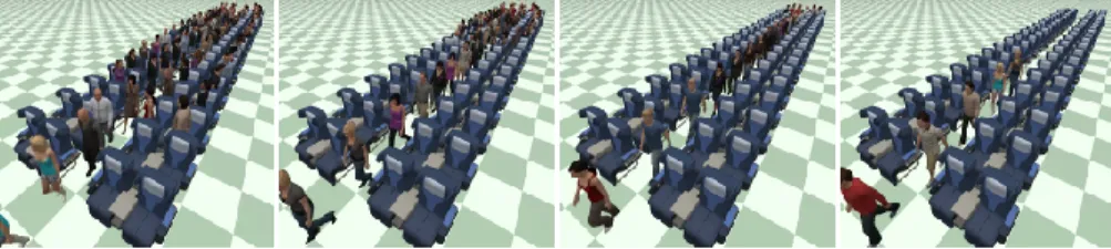
Figure 1: WarpDriver agents exiting a plane in seating order, solely due to collision avoidance, without additional scripting.
Abstract
1
Microscopic crowd simulators rely on models of local interaction 2
(e.g. collision avoidance) to synthesize the individual motion of 3
each virtual agent. The quality of the resulting motions heavily 4
depends on this component, which has significantly improved in 5
the past few years. Recent advances have been in particular due 6
to the introduction of a short-horizon motion prediction strategy 7
that enables anticipated motion adaptation during local interactions 8
among agents. However, the simplicity of prediction techniques of 9
existing models somewhat limits their domain of validity. In this 10
paper, our key objective is to significantly improve the quality of 11
simulations by expanding the applicable range of motion predic-12
tions. To this end, we present a novel local interaction algorithm 13
with a new context-aware, probabilistic motion prediction model. 14
By context-aware, we mean that this approach allows crowd sim-15
ulators to account for many factors, such as the influence of en-16
vironment layouts or in-progress interactions among agents, and 17
has the ability to simultaneously maintain several possible alternate 18
scenarios for future motions and to cope with uncertainties on sens-19
ing and other agent’s motions. Technically, this model introduces 20
“collision probability fields” between agents, efficiently computed 21
through the cumulative application of Warp Operators on a source 22
Intrinsic Field. We demonstrate how this model significantly im-23
proves the quality of simulated motions in challenging scenarios, 24
such as dense crowds and complex environments. 25
CR Categories: I.3.7 [Computer Graphics]: Three-Dimensional 26
Graphics and Realism—Animation; I.6.8 [Simulation and Model-27
ing]: Types of Simulation—Animation; 28
Keywords: crowd simulation, anticipation, collision avoidance 29
1 Introduction
30Much attention has recently been devoted to crowd simulation due 31
to its applications in pedestrian dynamics, virtual reality and digital 32
entertainment. As a result, many algorithms have been proposed 33
and they are typically separated into two main classes: macro-34
scopic algorithms that simulate crowds as a whole, and micro-35
scopic algorithms that model individual movement. Algorithms 36
of this second type can generate realistic individual agent trajec-37
tories and this capability is important for most crowd applications. 38
At their core, microscopic crowd simulators rely on the notion of 39
a local interaction model to formulate how agents influence each 40
other’s trajectory. The most required model of local interactions 41
deals with collision avoidance between agents which is the focus 42
of our paper. The quality of resulting simulations directly depends 43
on these models because, when numerous interactions occur such 44
as in crowds, they mostly determine how individual trajectories are 45
formed. As detailed in the next section, most recent approaches rely 46
on a short-term motion prediction mechanism in order to anticipate 47
motion adaptations during local interactions. They are referred to 48
as velocity-based algorithms as this prediction relies on the current 49
positions and velocities of agents. This new principle for interac-50
tion models allowed for significant progress in terms of realism at 51
both the local and global levels, because anticipation is observed in 52
humans. Despite these important advances, some issues persist and 53
have direct impact on simulation results. 54
Our hypothesis is that the persisting issues are due to a few basic 55
assumptions in the design of these local interaction models. In par-56
ticular, existing algorithms often assume that the current velocity of 57
agents is representative of their motion intent, and their motion pre-58
diction relies on the assumption of a constant velocity. Obviously, 59
the current velocity of agents could not always be representative of 60
their intent, for instance, when an agent turns or adapts its motion to 61
avoid collisions. Section 7 shows scenarios where prediction based 62
on simple linear motion extrapolation fails. Capturing a wider set 63
of observations on how each agent determines its motion, it is pos-64
sible to make more accurate motion predictions and consequently 65
to simulate more realistic local agent interactions. This realization 66
is the key insight in this paper. We propose a stochastic motion pre-67
diction model that accounts for the “context” of local agent-agent 68
and agent-environment interactions. 69
More precisely, two main aspects distinguish our solution from pre-70
vious ones. The first is our representation of future events. In pre-71
vious work, this is based on a simple linear extrapolation of each 72
agent’s current velocity. In our model, each agent constructs a (pos-73
sibly non-linear) probability field of colliding with other agents. 74
This representation is versatile, as it allows the crowd simulation 75
to maintain multiple possible future motions (more or less proba-76
ble) or to model various uncertainties due to sensing and human 77
behaviors in motion predictions. The second aspect is the model of 78
how agents react to this motion prediction. Given the probability 79
fields of collisions, the local collision response and avoidance can 80
be computed using a gradient descent on these fields. This solution 81
differs from macroscopic algorithms (e.g. [Treuille et al. 2006]), 82
whose density fields do not model agents’ future motions, sensing 83
uncertainties, or other agents’ responses. 84
In this paper, we introduce a generalized space-time local interac-85
tion model for crowd simulation using a unified, probabilistic the-86
oretic framework accounting for stochastic (and possibly nonlin-87
ear) motion prediction, non-deterministic sensing, and the unpre-88
dictability of human behaviors. Our main contributions include: 89
• A new collision avoidance algorithm that relies on a proba-90
bilistic prediction of each agent’s future motions. 91
• A technique to efficiently compute future collision probabili-92
ties thanks to an Intrinsic Field and Warp Operators; conse-93
quently, we refer to this algorithm as “WarpDriver”. 94
The rest of the paper is organized as follows. Section 2 provides 95
a brief review of related work and Sections 3, 4, 5, and 6 are de-96
voted to the technical description of our approach. In Section 7, we 97
demonstrate the benefits of our algorithm as compared to some of 98
the most recent algorithms, and discuss existing artifacts in highly 99
dense crowds, circulation in dynamic and complex environments, 100
and interactions with erratically-behaved agents. We show how this 101
new context-aware probabilistic motion prediction model can alle-102
viate many of these commonly known issues of existing simulation. 103
2 Related Work
104Much attention has recently been devoted to crowd simulation due 105
to its applications in pedestrian dynamics, virtual reality and cine-106
matic entertainment. Consequently, many crowd simulation algo-107
rithms, spanning several categories and each with its own charac-108
teristics, have been devised. Macroscopic crowd simulation algo-109
rithms [Narain et al. 2009; Treuille et al. 2006] animate crowds at 110
the global level, aiming to capture statistical quantities such as flows 111
or densities. In contrast, microscopic algorithms model interac-112
tions between individual pedestrians, with the emergence of move-113
ment patterns at the crowd level. For instance, algorithms based 114
on cellular automata discretize space into grids where pedestrians 115
are moved based on transition probabilities [Kretz and Schrecken-116
berg 2008; Schadschneider 2001]. Other, agent-based algorithms 117
model pedestrians as agents, with various levels of complexity. Fi-118
nally, example-based algorithms maintain databases of crowd mo-119
tions which can be reused depending on the context [Lerner et al. 120
2007; Ju et al. 2010]. 121
Among these works, agent-based algorithms remain very popular, 122
due to their ease of implementation and their flexibility through var-123
ious extensions and scripting. To reproduce local interactions be-124
tween people, these algorithms have always focused on the most 125
readily availabe and easily useable information: agents’ positions. 126
This has been the case starting with Reynolds’ seminal work with 127
the Boids algorithm [Reynolds 1987], later the Social-Forces algo-128
rithm by [Helbing and Moln´ar 1995; Helbing et al. 2000] and many 129
of their derivatives ever since. 130
However, anticipation of each other’s trajectories is key to peo-131
ple’s interactions, and efficient, collision-free navigation [Olivier 132
et al. 2012; Karamouzas et al. 2014]. In light of this observa-133
tion, major advances recently came from velocity-based algorithms. 134
[Reynolds 1999] introduced the point of closest approach between 135
agents, where, if the distance between the concerned agents was 136
to be low enough at this point (reflecting a collision), they would 137
steer away from it. Later, in an algorithm derived from Social-138
Forces, [Karamouzas et al. 2009] used this point of closest ap-139
proach as a source of repulsive forces; and [Pellegrini et al. 2009] 140
used the distance of the closest approach to refrain from choos-141
ing velocities which might lead to collisions. In parallel, other al-142
gorithms [Feurtey 2000; Paris et al. 2007] work in space-time (2-143
dimensional space plus one more dimension of time) to, again, se-144
lect permitted, collision-free velocities. This method of choosing 145
permissible velocities was further accelerated by algorithms that 146
reasoned in 2-dimensional velocity-space such as [van den Berg 147
et al. 2008; Guy et al. 2009; Guy et al. 2012a; Pettr´e et al. 2009]. 148
Most recently, [Karamouzas et al. 2014] introduced an algorithm 149
where velocity-based interactions are formulated as an optimiza-150
tion problem, the parameters of which are derived from observation 151
data, similarly to [Liu et al. 2005]. Finally, other algorithms used in-152
stantaneous velocities in other ways, such as affordance fields [Ka-153
padia et al. 2009] and velocity-derived values processed from the 154
synthetic visual flows of agents [Ondˇrej et al. 2010]. 155
As a common assumption, these algorithms all linearly extrapolate 156
agents’ future motions from their positions and velocities, mak-157
ing it possible to anticipate collisions up to a certain time hori-158
zon and improve simulation results [Olivier et al. 2012; Guy et al. 159
2012b; Wolinski et al. 2014]. However, this linear extrapolation 160
remains simplistic, and in many more challenging situations, does 161
not yield truly satisfactory results. Consequently, [Kim et al. 2014] 162
introduced a probabilistic component to the algorithm presented by 163
[van den Berg et al. 2008], while [Golas et al. 2013] added look-164
ahead to adaptively increase the time horizon in an efficient way 165
for large groups. Finally, [van den Berg et al. 2011a] incorporated 166
agents’ acceleration constraints into this same algorithm. 167
This underlying assumption of linear motion prediction, however, 168
does not hold in many cases, and we suggest that constraining a 169
crowd simulator to only information on positions and instantaneous 170
velocities is often insufficient. By addressing these issues, we intro-171
duce an approach that enables agents to efficiently take into account 172
arbitrary sources of information in a stochastic framework when an-173
ticipating each other’s future motions. 174
3 Overview
175Our algorithm builds on an agent-based modeling framework 176
and the resulting simulator captures complex interactions among 177
agents. In this section, we provide a high-level overview (Figure 2) 178
of our approach, i.e. how we model interactions between agents 179
and steer them. However, before describing “WarpDriver”, we first 180
need to define what we consider an agent in our formulation. An 181
agent is any entity that the algorithm would steer or any other entity 182
that could affect another agent’s steering decisions. Agents can be, 183
for instance, pedestrians, cars or walls, and they can further have 184
various properties: size, shape, position, velocity, followed path, 185
etc. In addition, in our formulation, interactions between agents are 186
resolved in space-time. To simulate these interactions, we identify 187
the perceiving agent (the agent we are currently steering) and the 188
perceived agents (the agents that are to be avoided). Interactions 189
among agents are modeled in three main steps: 190
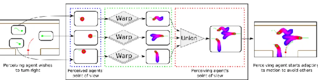
Step 1, Setup: The perceiving agent starts by defining its space-191
time projected trajectory: the trajectory it would follow if no 192
collisions were to happen (red dotted line on left of Figure 2 193
and Figure 3; detailed in Section 4). 194
Step 2, Perceive: This agent then constructs its perception of other 195
perceived agents’ future motions in the form of space-time 196
collision probabilities (middle of Figure 2 and color gradient 197
on Figure 3; detailed in Section 5). 198
Step 3, Solve: Finally, the agent intersects its projected trajectory 199
with these collision probabilities (thus evaluating the chances 200
of collision along the projected trajectory) and modifies its 201
projected trajectory by performing one step of gradient de-202
scent to lower its collision probabilities along this trajectory 203
(green dotted line on right of Figure 2 and Figure 3; detailed 204
in Section 6). 205
The most important aspect of our approach is then how the perceiv-206
ing agent derives collision probabilities from the perceived agents. 207
It is through this process that we can model any non-linear behavior 208
of both perceiving and perceived agents. 209
Figure 2: Overview of the algorithmic framework of WarpDriver.
Figure 3: Illustration of collision avoidance between two agents a and b on a curved path. The color gradient represents a’s prob-ability of collision with b, as perceived by a. The red dotted line represents a’s initial projected trajectory. The green dotted line represents a’s final, corrected, projected trajectory (exaggerated). The red line in between both dotted ones represents the correction agent a will perform (exaggerated for illustration). Note that the projected trajectory is a curve path due to Warp Operators. Our goal for the collision probability formulation process (Step 2) 210
is to be able to handle each property separately. Thus, we define 211
the Intrinsic Field as the lowest common denominator among all 212
agents: the fact that they occupy a volume in space-time (they co-213
exist); this is a collision probability field. We then model any addi-214
tional property as a Warp Operator which further warps the Intrin-215
sic Field. 216
In order to define a clean system pipeline for implementation, we 217
further associate every agent with its own agent-centric space-time. 218
Step 2 is then described by the following three sub-steps: 219
• Every perceived agent is modeled as an Intrinsic Field in its 220
agent-centric space-time (blue rectangle in Figure 2). 221
• Warp Operators progressively warp every perceived agent’s 222
Intrinsic Field from its agent-centric space-time into the per-223
ceiving agent’s agent-centric space-time (green rectangle in 224
Figure 2). 225
• These warped collision probability fields (in the perceiving 226
agent’s agent-centric space-time) are then combined into a 227
single collision probability field (red rectangle in Figure 2). 228
Note that by confining agents’ properties to Step 2, the perceiv-229
ing agent’s projected trajectory can be simply defined as a line in 230
its agent-centric space-time, which simplifies further computations 231
(more detail in Sections 4, 6). 232
4 Notations and Setup
233In this section, we describe the notations used throughout the paper 234
and detail how a perceiving agent constructs its projected trajec-235
tory, i.e. its current trajectory in space-time assuming no collisions 236
take place (Step 1 of our approach, see Figure 2): 237
• ·,×, ◦, � and ∗ respectively denote the dot product, cross 238
product, function composition, component-wise multiplica-239
tion and convolution. 240
•−→∇ is the nabla operator. For a continuous field f,−→∇ · f is the 241
gradient of f. 242
• ∪ is the union operator and�is the union operator over a set. 243
• A is the set of all agents, a, b ∈ A are two such agents; note 244
that a usually denotes the perceiving agent while b usually 245
denotes the perceived agent. 246
• S is a 3D space-time with basis {x, y, t}, where x and y 247
form the space of 2D positions and t is the time. A point 248
in such a space-time is noted s = (x, y, t) ∈ S. Note the 249
difference between bold-face vectors (e.g. x) and normal-font 250
scalar quantities (e.g. x). 251
• Sa,kis the agent-centric space-time S centered on an agent
252
aat timestep k such that, in this space-time, agent a is at 253
position o = (0, 0, 0) ∈ Sa,kand faces along the local x
254
axis, positive values along the local t axis represent the future. 255
• ra,kis agent a’s projected trajectory in Sa,k.
256
• ∀s ∈ Sa,k, pa→b,k(s)is what agent a perceives to be its
257
collision probability with agent b. 258
• I, the Intrinsic Field, gives the probability of colliding with 259
any agent b in space-time Sb,k. −→∇ · I is the gradient of I.
260
• W denotes a Warp Operator that warps I for every property of 261
an agent. W = Wn◦...◦W1further denotes the composition
262
of operators {W1, ..., Wn}.
263
• W−1is used to apply the inverse of a Warp Operator W to
probabilities and probability gradients. Assuming a collec-tion of operators {W1, ..., Wn} where W(Sa,k) =Sb,k, then
W−1= W−1 1 ◦ ... ◦ Wn−1and ∀s ∈ Sa,k: (W−1◦ I ◦ W)(s) = p a→b,k(s), (1) (W−1◦ (−→∇ · I) ◦ W)(s) =−→∇ · p a→b,k(s). (2)
With these notations, in Step 1 of our approach, the perceiving agent 264
aconstructs its projected trajectory ra,kin its agent-centric
space-265
time Sa,k. We further assume that the perceiving agent a is a point
266
in its agent-centric space-time, Sa,kis then its configuration-space.
267
As mentioned in Section 3, since the processing of agents’ proper-268
ties is confined to Step 2, the perceiving agent’s projected trajectory 269
can be defined as a line. 270
Specifically, assuming agent a has an instantaneous speed va,k
271
at timestep k, its projected trajectory is expressed as ra,k =
272
line(o, va,kx + t). Further, at any time t ∈ R in the future, the
273
perceiving agent a projects to be at point ra,k(t) = o+t(va,kx+t)
274
in space-time Sa,k.
275
5 Perception: collision probability Fields
276We here describe how the perceiving agent constructs collision 277
probabilities from the perceived agents. As mentioned in Section 3, 278
this is a three-step process where: 279
• the Intrinsic Field I is defined for each perceived agent b in 280
its agent-centric space-time Sb,k,
281
• Warp Operators warp I from each Sb,kinto the
perceiv-282
ing agent a’s agent-centric space-time Sa,k, thus modeling
283
agents’ properties, 284
• the resulting collision probability fields are combined. 285
We detail each of these three steps in the following sub-sections. 286
5.1 The Intrinsic Field
287
As defined in Section 3, the Intrinsic Field is the lowest common 288
denominator between agents, independently of their properties. It 289
is also a continuous collision probability field: for each point s in a 290
perceived agent b’s agent-centric space-time Sb,k, it gives the
prob-291
ability of colliding with b at that point I(s) ∈ [0, 1]. 292
Since the perceiving agent a is a point in its agent-centric configuration-space Sa,k, any perceived agent b should therefore
be perceived as a configuration-space obstacle (the Minkowski sum of agents a and b). As we want the Intrinsic Field to be indepen-dent of agents’ properties (including size and shape) we define the Minkowski sum of agents a and b as a disk with a normalized radius of 1, this is the step function g:
∀s = (x, y, t) ∈ Sb,k, g(s) =
�
1, if�x2+ y2≤ 1
0, otherwise
We further model the perception error in the form of a Gaussian 293
function: ∀s = (x, y, t) ∈ Sb,k, f (s) = exp(−(x
2+y2
2σ2 )).
294
Consequently, we define the Intrinsic Field as the convolution of 295
functions f and g: 296
∀s ∈ Sb,k, I(s) = (f∗ g)(s). (3)
It is computed up to a normalized time of 1 second in the future. An 297
illustration of the Intrinsic Field can be found on Figure 2 (cylinder 298
on the right side of the figure). 299
5.2 Warp Operators
300
Warp Operators model each agent property that we want to include 301
in the algorithm. As mentioned in Section 3, these could be: shape, 302
size, position, velocity, followed path, etc. Mechanically, Warp Op-303
erators warp the Intrinsic Field defined for each perceived agent 304
bin its agent-centric space-time Sb,kinto the perceiving agent a’s
305
agent-centric space-time Sa,k.
306
In this sub-section, we describe Warp Operators modeling agent-307
related and context-related properties. Note that their formal ex-308
pressions are given in Appendix A. 309
5.2.1 Agent-Related Operators
310
The following Warp Operators model properties which only de-311
pend on agents: 312
Position and Orientation The Warp Operator Wlocalmodels the
313
agents’ position and orientation properties. It is a simple 314
change of referential between Sa,kand Sb,k.
315
Time Horizon To avoid collisions in a time horizon T (beyond the 316
normalized 1 second in the Intrinsic Field), we define a time 317
horizon operator Wth.
318
Time Uncertainty The Wtuoperators models the increased
un-319
certainty on the states of other agents the further we look in 320
time. 321
Radius The Wroperator changes the radius of the agents by
dilat-322
ing space along the x and y axes. 323
Velocity The Wvoperator models the agent’s instantaneous
veloc-324
ity as a displacement along the x axis. 325
Velocity Uncertainty Depending on the speed of an agent, that 326
agent could be more or less likely to make certain adaptations 327
to its trajectory. For instance, the faster an agent travels, the 328
more likely it is to accelerate/decelerate rather that turn. This 329
is modeled by the Wvuoperator.
330
5.2.2 Context-Related Operators
331
The following operators provide information based on the Envi-332
ronment Layout (operator Wel), Interactions with Obstacles
(op-333
erator Wio) and Observed Behaviors of agents (operator Wob).
334
These operators, where applicable,replace the Local Space op-335
erator Wlocal. We call Wrefthe resulting operator: Wref =
336
{Wlocalor Welor Wioor Wob}.
337
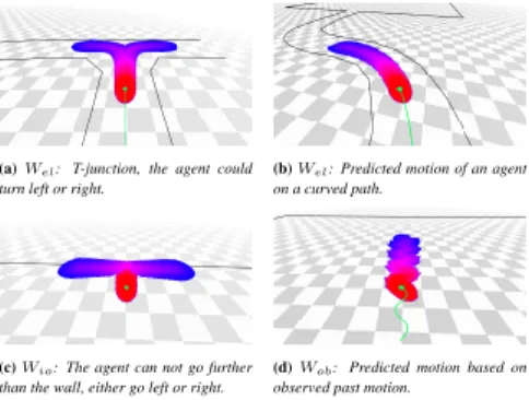
(a) Wel: T-junction, the agent could
turn left or right.
(b) Wel: Predicted motion of an agent
on a curved path.
(c) Wio: The agent can not go further
than the wall, either go left or right.
(d) Wob: Predicted motion based on
observed past motion.
Figure 4: Cases using context-related Warp Operators (Sec-tion 5.2.2). Each case represents one context-related Warp Oper-ator combined with all agent-related ones (Section 5.2.1). Same simplified 2D representation as in Figure 3(right).
Environment Layout When navigating in an environment, based 338
on its layout, we can predict what trajectories other pedestrians 339
are likely to follow. In a series of hallways, for instance, when 340
not threatened by collisions with other pedestrians, one would stay 341
roughly in the middle of the hallway and take smooth turning tra-342
jectories at intersections (an agent could turn either left or right in 343
Figure 4a). When navigating on curved paths, one would, again, 344
have a tendency to stay roughly in the middle, resulting in a curved 345
trajectory (Figure 4b). The operator Welmodels this knowledge by
346
warping space to “align” it with these probable trajectories. 347
Interactions With Obstacles Where the environment layout op-348
erator focuses on other agents’ probable trajectories assuming they 349
will continue travelling, this operator Wiotakes care of possible
350
interactions between agents and obstacles. These interactions are 351
essentially much more drastic changes to an agent’s locomotion 352
than paths, such as full stops. These can occur if, for instance, 353
an agent comes up to a wall (Figure 4c) (to interact with an ATM, 354
look out the window, check a map...). This can also happen with an 355
agent coming into contact with a small/temporary/unexpected ob-356
stacle which could force it to stop and then “hug” the obstacle to 357
get around it. 358
To achieve this, we construct a graph around each obstacle (an ob-359
stacle being modeled as a series of connected line segments). When 360
an agent’s projected trajectory intersects with an obstacle, we ex-361
tend the graph to that agent and “align” space-time wih this graph. 362
Observed Behaviors With the last operator Wob, we aim to
im-363
prove the prediction of agents’ future motions by looking at their 364
past ones. In the worst case, we might not find any useful informa-365
tion, which won’t impact the prediction. However, we might also 366
find some behaviors similar to what the agent is currently doing 367
(e.g. turning in a particular way) or, in the best case, we might find 368
patterns (e.g. agents going in near-circles, zig-zags...) that we can 369
extend to the currently-observed situation (Figure 4d shows antici-370
pation on a zig-zagging agent). 371
In order to take this information into account for an agent a at 372
timestp k, we keep a history of this agent’s positions during h previ-373
ous timesteps. These past positions form a graph which we repeat 374
on the current position of the agent and then “align” space-time 375
with it. 376
5.2.3 Composition of Warp Operators
377
As defined in Section 3, we can compose all these operators {Wref, Wth, Wtu, Wr, Wv, Wvu}:
W = Wref◦ Wth◦ Wtu◦ Wr◦ Wv◦ Wvu,
W−1= W−1
vu◦ Wv−1◦ Wr−1◦ Wtu−1◦ Wth−1◦ Wref−1.
For any point s in perceiving agent a’s agent-centric space-time Sa,k:
pa→b,k(s) = (W−1◦ I ◦ W)(s),
− →
∇ · pa→b,k(s) = (W−1◦ (−→∇ · I) ◦ W)(s).
5.3 Combining collision probability Fields
378
Before the collision avoidance problem can be solved, one last me-chanic still needs to be defined which is how pair-wise interactions can be combined (Step 3 on Figure 2). Let a be the perceiving agent, and b, c ∈ A, b �= a, c �= a be a pair of perceived agents. At timestep k, we have access to the following collision probabilities: pa→b,kand pa→c,k. We can then define the probability agent a has
of colliding with either b or c:
pa→{b,c},k= pa→b,k+ pa→c,k− pa→b,kpa→c,k.
And we can similarly define its gradient: −
→
∇ · pa→{b,c},k=−→∇ · pa→b,k+−→∇ · pa→c,k
− pa→b,k−→∇ · pa→c,k
− pa→c,k−→∇ · pa→b,k
Finally, considering the whole set of agents A, the probability agent 379
ahas of colliding with any other agent b ∈ A \ a is obtained in the 380
same manner and noted pa→A\a,k, with the corresponding gradient
381 − →∇ · p
a→A\a,k.
382
6 Solving the Collision-Avoidance Problem
383This section details the third and final step in our approach: how 384
the perceiving agent modifies its projected trajectory to reduce the 385
collision probabilities along it. 386
To solve the collision-avoidance problem, the perceiving agent 387
samples collision probabilities and their gradients pa,kalong its
388
projected trajectory ra,k(this is the cost function and its gradient),
389
and performs one step of gradient descent to modify its projected 390
trajectory. First, we compute the overall probability an agent a has 391
of colliding with other agents pa,k, its gradient −→∇ · pa,kand
appli-392
cation point sa,k(red continuous line in Figure 3), when traveling
393
along its projected trajectory ra,k(red dotted curve in Figure 3).
394
We compute these quantities for a time horizon T∗until a collision
395
with a wall is detected: T∗≤ T . With the following normalization
396
factor Na,k, and t ∈ [0, T∗]:
397
Na,k=
�
t
pa→A\a,k(ra,k(t)), (4)
We compute pa,k, −→∇ · pa,kand sa,k:
pa,k= 1 Na,k � t pa→A\a,k(ra,k(t))2, (5) − →∇ · p a,k= 1 Na,k � t
pa→A\a,k(ra,k(t)) (−→∇ · pa→A\a,k)(ra,k(t)),
(6) sa,k= 1 Na,k � t
pa→A\a,k(ra,k(t)) ra,k(t). (7)
From these quantities, given a user-set parameter α, we compute 398
the new projected trajectory that agent a should follow in Sa,kto
399
lower its collision probability (green dotted curve in Figure 3) : 400
r∗
a,k= line(o, sa,k− αpa,k−→∇ · pa,k). (8)
7 Results
401
In this section, we show the benefits of our WarpDriver algo-402
rithm as compared with several existing methods. To illustrate 403
the advantages of the more complex Warp Operators, we compare 404
WarpDriver with two velocity-based algorithms: the well-known 405
ORCA algorithm [Van Den Berg et al. 2011b] and the recent Pow-406
erlaw algorithm [Karamouzas et al. 2014], as they are representa-407
tive of what can be achieved with velocity-based approaches. We 408
also compare WarpDriver with two position-based algorithms: the 409
Boids [Reynolds 1987] and the Social-Forces [Helbing and Moln´ar 410
1995] algorithms. 411
First, we test WarpDriver in challenging scenarios, including large, 412
dense crowds, scenarios with non-linear routes, history-based an-413
ticipation cases and a highly-constrained situation. We show the 414
results of our algorithm vs. Powerlaw, ORCA, and Social-Forces 415
(Boids is omitted here, as in these situations it gives largely similar 416
results as Social-Forces). Second, we present benchmark results on 417
previously studied data sets for all five algorithms, as well as details 418
on the algorithmic performance of WarpDriver. 419
Finally, several of the shown values are measured over the dura-420
tion of the simulated scenarios for each algorithm; in the interest of 421
space, we show these results in a compact way (violin plots, box-422
plots); the corresponding full graphs can be found in Appendix B. 423
7.1 Large and Dense Crowds
424
Figure 5: Big Groups example: two groups of 1027 agents each are made to traverse each other. Simulated with WarpDriver.
Figure 6: Crossing example: two flows of agents in corridors cross each other at a right angle (red ones going to the top and blue ones going to the right). Simulated with WarpDriver.
Figure 7: Issues encountered in Big Groups and Crossing. Left: Big Groups, ORCA agents block each other. Right: Crossing, con-gestion observed for Powerlaw.
We start with simulation tests involving a large number of agents 425
and high densities (agents are within contact distance of each other), 426
testing our algorithm’s ability to navigate agents while subject to 427
many, simultaneous interactions. 428
7.1.1 Description
429
Test case 1: Big Groups This first test case involves two 1027-430
agent groups exchanging positions as seen on Figure 5. In this kind 431
of example, we expect agents to be able to traverse through the op-432
posing group (ideally with the formation of lanes) and reach their 433
destinations. This expected behavior implies a certain level of or-434
ganization of the agents; thus we measure how many sub-groups 435
emerge (using the method from [Zhou et al. 2012]) and how widely 436
agents might spread (Figure 8, top and bottom respectively). 437
Test case 2: Crossing The second test case involves two corri-438
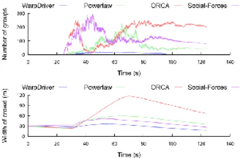
dors intersecting at a right angle, each with a uni-directional flow 439
Figure 8: Top: number of emerging sub-groups, low for Warp-Driver (i.e. number of lanes), high for all other algorithms. Bottom: spread of agents, WarpDriver agents stay compact, other agents spread widely.
Figure 9: Top: number of jammed agents, close to none for Warp-Driver, many for other algorithms. Bottom: violin plots of detected agent lines at crossing intersection, consistently around −45◦for
WarpDriver, scattered (and fewer detected lines) for other algo-rithms; full graphs in Appendix B.
of agents (Figure 6). This kind of situation is well studied and 440
45◦lines should form between agents of each flow at the
intersec-441
tion [Cividini et al. 2013], facilitating their movement. We measure 442
this by detecting sub-groups with the previously mentioned method 443
and perform linear regression on the agents, results are reported 444
on Figure 9(middle, bottom). Furthermore, as the situation is very 445
constrained (agents at contact distance from each other with the 446
presence of walls), we also measure how many agents are jammed 447
(travel at less than 0.1m/s) during the simulations, as shown in Fig-448
ure 9(top). 449
7.1.2 Analysis
450
Big Groups In the Big Groups example (Figure 5), agents sim-451
ulated with our algorithm are able to do two things. First, front-452
line agents are able to find points of entry in the opposing group 453
(which correspond to the minima of the collision probability func-454
tion) and consequently enter through them. Second, non-front-line 455
agents are able to anticipate the front-liners’ continuing motion and 456
align themselves behind them. In the resulting motion, agents re-457
organize themselves into lanes and are able to fluidly reach their 458
destinations. This re-organization can be observed through the low 459
number of emerging sub-groups (Figure 8(top)) which correspond 460
to the formed lanes, and through the relatively low spread of the 461
agents (Figure 8(bottom)). 462
In the case of the other algorithms, however, the groups can be ob-463
served to collide, block each other, and spread in order to allow 464
agents (individual or in small groups) to pass through to their goals 465
(a still of this can oberved on the left of Figure 7). For the ORCA 466
algorithm, for example, this is due to the solution space quickly be-467
coming saturated, thus forcing the agents to start spreading on the 468
sides in order to free up the velocity space and be able to continue 469
their motion. This disorganization can be observed through the high 470
number of emerging sub-groups (Figure 8(top)) corresponding to 471
agents searching for a less saturated solution space, thereby spread-472
ing over larger distances (Figure 8(bottom)). 473
Crossing In the Crossing situation (Figure 6), as expected agents 474
simulated with our algorithm are able to cross without congestion 475
(Figure 9, top: no jammed agents) forming the expected 45◦
cross-476
ing patterns (Figure 9, bottom). 477
Other algorithms’ agents on the other hand, as can be seen on the 478
right of Figure 7 quickly get into a congestion (Figure 9, top: in-479
creasing numbers of jammed agents) and no consistent patterns can 480
be found, as seen on the bottom of Figure 9. 481
Summary Overall, WarpDriver is able to better find (and take 482
advantage of) narrow spaces between agents (local minima in the 483
collision probability fields) thus producing more visually pleasing 484
results than the other algorithms, which often have more binary re-485
actions, leading to entrapping agents in congested scenes. 486
7.2 Non-Linear Motion
487
Figure 10: Curved Flows example: two opposite flows of agents on a curved path (blue ones turn clockwise, red ones counter-clockwise). Simulated with WarpDriver.
Figure 11: Curved Obstacle example: a small obstacle is on the way of a flow of agents on a curved path. Simulated with Warp-Driver.
With the following test cases, we investigate how our algorithm 488
copes with situations where agents’ future motions are non-linear. 489
To this end, we make agents interact with each other and with ob-490
stacles, while traveling along curved paths. 491
Figure 12: Issues encountered in Curved Flows and Curved Ob-stacle. Left: Curved Flows, congestion observed for ORCA. Right: Crossing, Powerlaw agents can only pass the obstacle on their right.
Figure 13: Agent speeds in straight vs. curved corridors (same corridor length and width, same agent density). WarpDriver: con-sistent agent motions; other algorithms’: important loss of speed in curved corridor. Full graphs in Appendix B.
7.2.1 Description
492
Test case 3: Curved Flows In this situation (Figure 10), we set 493
two opposing flows of agents (moderate density, about a meter be-494
tween agents) in a curved corridor. Here, with the moderate density, 495
we expect agents to fluidly navigate to the other end of the corridor. 496
To measure the impact the curved corridor has on the agents, we re-497
produced the experiment in all aspects (same number and density of 498
agents, same corridor length and width) except for one: we made 499
the corridor straight. We then measured the average speed of the 500
agents first in the straight version and then in the curved version, as 501
seen in Figure 13. 502
Test case 4: Curved Obstacle This situation is a simplification 503
of the previous test case: one uni-directional flow of agents is made 504
to travel the same curved corridor with one small obstacle in the 505
middle as shown on Figure 11. In this simple test case, we expect 506
Figure 14: Agent traces. WarpDriver agents pass the obstacle on the most convenient side. Social-Forces agents bump on the obsta-cle and pass on closest side. Powerlaw and ORCA agents can only pass on their right (some ORCA agents get pushed to left side by a small congestion).
the agents to easily bypass the obstacle on the side that is most 507
direct, i.e. if an agent is on the outer (resp. inner side) side of the 508
corridor it should bypass the obstacle on the outer side (resp. inner 509
side). We thus looked at the paths agents followed (Figure 14). 510
7.2.2 Analysis
511
Curved Flows In the Curved Flows example (Figure 10), agents 512
simulated with our algorithm are able to avoid each other correctly, 513
with the emergence of a few opposing lanes which facilitate flow. 514
Furthermore, in Figure 13 we can see that using our algorithm, 515
agents travel at the same overall speed in both the straight and 516
curved versions. 517
With the other algorithms on the other hand, agents quickly get 518
stuck in a congestion (Figure 12, left). We can observe this in 519
Figure 13, which shows an important loss of agents’ speed on the 520
curved version of the corridor as compared to the straight one. 521
Curved Obstacle The Curved Obstacle situation shows the phe-522
nomenon more clearly. With our algorithm, agents anticipate the 523
obstacle about 3m in advance (see Figure 14, top left) and choose 524
the most direct (expected) side. 525
Agents from the Powerlaw and ORCA algorithms on the other hand 526
can be seen to all prefer the outer side (with respect to the curve) of 527
the obstacle (Figure 14, top right and bottom left) and some agents 528
backtrack (Figure 14, top right) and use the inner side when a bot-529
tleneck situation forms. The Social-Forces algorithm produces re-530
sults analogous to ours (Figure 14, bottom right): being position-531
based, this algorithm steers agents without anticipation and thus 532
they “bump” on the obstacle and pass it on this same side. 533
Summary In both examples, the difference between our algo-534
rithm and the two velocity-based algorithms is that agents simu-535
lated with WarpDriver anticipate their own (and others’) future tra-536
jectories as curved along the corridor, thus perceiving interactions 537
where they most probably will occur (thus they see agents in the op-538
posite flow and obstacle from the two examples well in advance). 539
Velocity-based agents in these cases exhibit visual artifacts due to 540
their linear extrapolation of trajectories based on instantaneous ve-541
locities: they can only perceive interactions that will occur roughly 542
on a line tangent to the corridor curve at their position (thus they do 543
not react in advance to agents in the opposite flow nor the obstacle 544
from the two previous examples until the very last moment). 545
7.3 History-based Anticipation
546
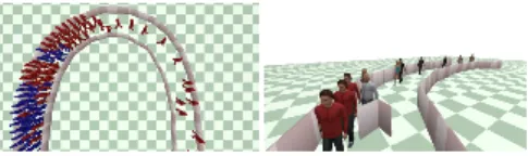
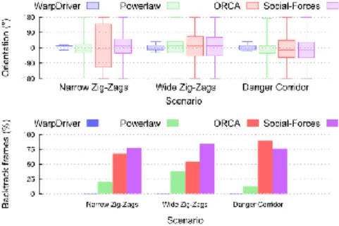
Figure 15: Zig-Zags example: agents (blue) avoid a zig-zagging agent (red); left: narrow zig-zags, right: wide zig-zags. Simulated with WarpDriver.
As instantaneous velocities can vary very rapidly and not be repre-547
sentative of agents’ overall motions, we next test situations where 548
agents or obstacles behave according to pattern-like movements. 549
We test two easily-recognizable behaviors: zig-zagging and revolv-550
ing motions. 551
Figure 16: Danger Corridor example: agents (blue) avoid turning obstacles (red). Simulated with WarpDriver.
Figure 17: Issues encountered in Zig-Zags and Danger Corridor. Left: Zig-Zags, powerlaw agents backtrack from zig-zagging agent. Right: Danger Corridor, ORCA agents backtracking and perform-ing other erratic motions next to turnperform-ing obstacles.
7.3.1 Description
552
Test case 5: Zig-Zags In this scenario (Figure 15), we set up a 553
uni-directional flow of moderately-spaced agents (in blue) traveling 554
along a straight corridor and further add an agent (in red) which 555
travels counter-flow with a zig-zagging trajectory. Figure 15 shows 556
both cases where the red agent has a narrow zig-zagging motion 557
(left) as well as a wide motion (right). In this example, we expect 558
the blue agents to recognize and anticipate the red one’s motion 559
pattern and easily avoid it. We measured how easily blue agents 560
are able to avoid the red one by recording the angle between the 561
agents’ orientation and their goal direction (their deviation from 562
their goal) on Figure 18(top). We also report what proportion of the 563
simulated frames contain backtracking agents (180◦deviations) on
564
Figure 18(bottom). 565
Test case 6: Danger Corridor This scenario (Figure 16) is 566
largely similar to the previous one in that a uni-directional flow 567
of agents (in blue) travel down a corridor, except that we set nine 568
slowly revolving pillars (in red) in the middle of the path. We then 569
expect agents to be able to recognize how these pillars move and 570
easily work out a path through them. Again, we measure the agents’ 571
deviation from their goals which we report on Figure 18(top) and 572
the proportion of frames containing backtracking agents on Fig-573
ure 18(bottom). 574
7.3.2 Analysis
575
Zig-Zags In the Zig-Zag examples (Figure 15), agents (in blue) 576
simulated with WarpDriver are able to anticipate the zig-zagging 577
agent (in red) in advance and minimally adapt their trajectories to 578
avoid it. This is confirmed by Figure 18(top) which shows that the 579
heading direction of the agents is very close to 0◦(heading in their
580
preferred direction). 581
Other algorithms’ agents, on the other hand, have more trouble an-582
ticipating the jerky motion of the zig-zagging agent and noticeably 583
over-react as a result. This is confirmed by the large spreads of 584
boxplots from Figure 18(top) where agents often deviate by ±180◦
585
(i.e. backtracking from their goal, as seen on Figure 18(bottom)). 586
Danger Corridor The Danger Corridor example (Figure 16) 587
yields results largely similar to the Zig-Zags one (but more pro-588
nounced). WarpDriver agents are able to fluidly avoid the revolving 589
obstacles with similarly little deviation (as for the Zig-Zags) from 590
Figure 18: Top: orientation of agents with respect to intended di-rection. WarpDriver agents are able to consistently head towards their intended direction. Other algorithms’ agents make very strong adaptations to their motions. Full graphs in Appendix B. Bottom: percentage of simulated frames containing backtracking agents; No WarpDriver agent has been backtracking. Other algorithms con-tain many backtracking agents.
their goal direction (Figure 18(top)). 591
Other agents have, again, more trouble dealing with the situation, 592
with much larger deviations from their intended directions (Fig-593
ure 18(top)), and a noticeable amount of backtracking agents (Fig-594
ure 18(bottom)). Non-similarly to the Zig-Zags however, in the case 595
of the Danger Corridor, the Powerlaw algorithm produced many 596
collisions between the agents and the revolving obstacles (a colli-597
sion is found when the center of an obstacle is inside the radius of an 598
agent; 21% of the simulation frames contained collisions for Pow-599
erlaw, as compared to less than 0.5% for ORCA and Social-Forces 600
and 0% for WarpDriver). 601
Summary Overall, the differences can be explained by the fact 602
that in these cases, the instantaneous velocities of the zig-zagging 603
agent and revolving obstacles are constantly changing and their tra-604
jectories are not straight. Thus, velocity-based algorithms first lin-605
early extrapolate (incorrect) future motions and then face these ex-606
trapolations constantly changing. The resulting agents thus avoid 607
many, ever-changing and possibly non-existent future interactions, 608
with large deviations from their intended directions and many 609
agents backtracking away from their goal. 610
These artifacts are addressed by WarpDriver: first, it detects pat-611
terns in the past motions and learns from them to anticipate fu-612
ture motions; second, when anticipating future motions it does so 613
non-linearly. As a result, WarpDriver agents are able to correctly 614
anticipate and avoid collision with other agents, resulting in more 615
natural reaction by agents (low deviation from intended directions) 616
and none of them back-tracking. 617
7.4 Highly-Constrained Space
618
Figure 19: Plane example: plane exit situation involving 80 agents. Simulated with WarpDriver.
Figure 20: Issues encountered in Plane: Powerlaw agents from aisle seats exit before everyone else.
Figure 21: Kendall tau coefficient for plane exit order, higher is better. WarpDriver produces an order very close to the expected one, while other algorithms produce much further orders. In the last scenario, we test our algorithm on coping with highly-619
constrained scenarios, as in very confined spaces, where agents are 620
within contact distance and many encounter path intersections. 621
7.4.1 Test case 7: Plane
622
This example features a plane egress scenario with 80 agents (Fig-623
ure 1 and Figure 19). Here, we expect agents to orderly exit the 624
plane starting with the ones close to the exit and with more far-625
away agents exiting last. To see how agents are able to cope with 626
this situation, we assigned to each agent the number of its row (e.g. 627
the four agents of the first row have the number 1, the four agents of 628
the last row have the number 20), then we recorded the number se-629
quence of agents as they got out of the plane and compared it using 630
the Kendall tau measure [Kendall 1938] to the ideal exit sequence 631
[1, 1, 1, 1, ..., 20, 20, 20, 20](Figure 21). 632
7.4.2 Analysis
633
As can be seen on Figure 19, with our algorithm, agents in the back 634
allow agents up front to exit first. This behavior leads to an orderly 635
exiting process, where all agents are progressively evacuated, as 636
evidenced by the high Kendall tau coefficient (0.96) which indicates 637
the exit sequence is close to the ideal one Figure 21. The behavior 638
obtained with our algorithm results from a combination of factors. 639
First, agents are able to predict which way the others will go: into 640
the alley and then towards the exit (note that these paths are non-641
linear since they contain a right turn). Second, agents in the front 642
rows are closer to the exit than the others and they are thus perceived 643
as obstacles blocking the exit from the other agents (and conversely 644
front agents perceive other agents as being “behind”), thus creating 645
a hierarchy. Finally, the agents easily navigate between the chairs 646
by following the local minima of the collision probabilities defined 647
by these obstacles. 648
On the contrary with the other algorithms, all agents try to exit at the 649
same time which, with the very constrained space (little room for 650
maneuvers) leads to unorderly behaviors. For instance, in the case 651
of the Powerlaw algorithm (Figure 20), aisle agents all gather in the 652
alley at the same time and exit before everyone else; while the alley 653
agents exit, window agents from the back have more space and exit 654
next; overall, window agents from the front and middle rows are 655
last to exit. This general lack of order is further confirmed by the 656
much lower Kendall tau values for Powerlaw, ORCA and Social-657
Forces found in Figure 21. In order for these algorithms’ agents to 658
exit in order, additional scripting would be required. 659
7.5 Benchmarks
660
Previous results provide a quantitative evaluation of visual artifacts, 661
including comparisons with previous techniques; this section pro-662
vides additional evaluation of results along two aspects: compar-663
isons with real data and an analysis of algorithmic complexity and 664
computational performance. 665
Figure 22: Benchmarks results using the method from [Wolinski et al. 2014], lower is better.
Data-driven validation Finally, we compared our algorithm’s 666
performance with the Powerlaw, ORCA, Social-Forces, and Boids 667
algorithms on previously-studied test cases using the method 668
from [Wolinski et al. 2014]. In these tests, the difference between 669
our algorithm and the others is not always as pronounced as in the 670
previously shown scenarios. This is due to the nature of the avail-671
able ground truth data which only captures simple interactions: (1) 672
simple crossing situations between 2-5 agents, and (2) 6-24 agents 673
exchanging positions on a circle. Nonetheless, as Figure 22 shows, 674
on these test cases, our method (in blue) gives comparable results 675
to velocity-based algorithms (Powerlaw - green, and ORCA - red), 676
occasionally outperforming them (and almost always outperform-677
ing the other algorithms). 678
Complexity Like for most other simulation algorithms, the base 679
complexity of our approach is quadratic, O(n2): every agent
inter-680
acts with every other agent. Most algorithms deal with this using 681
space-optimization structures such as kd-trees that reduce the run-682
time complexity by limiting the number of neighbors for a given 683
agent, but with the possible risk of arbitrarily discarding important 684
agents and thereby degrading results. 685
While we could also use such a strategy for WarpDriver, we note 686
that it is algorithmically very close to ray-tracing. We can thus bor-687
row strategies from the wide associated literature, such as parallel 688
sampling, caching, level-of-detail, etc. We have implemented one 689
such strategy, where in a pre-processing phase at the start of each 690
timestep, each agent imprints a theoretical maximum bounding vol-691
ume of its associated collision probability field onto a grid. Then, 692
when an agent samples collision probabilities, instead of sampling 693
every other agent’s field, it only samples the fields of those that 694
have their ID imprinted at that location on the grid. As a crowd 695
is not infinitely compressible, there is a maximum number of inter-696
actable neighboring agents, thus giving our algorithm a linear upper 697
bound to its complexity of O(n). This technique allows us to have 698
the same simulations with and without it: i.e. we can optimize the 699
runtime complexity without degrading the simulation results. 700
In practice, assuming the typical target framerate of 15-20 fps for 701
the motion of crowds, our algorithm can simulate 5, 000 agents in 702
real time. In comparison, on the same machine and for the same 703
number of agents, ORCA runs at ∼140 fps. Powerlaw on the other 704
hand, for stability reasons requires much lower timesteps – values 705
of ∼0.005 sec can be found in the examples bundled with the source 706
code, which means it needs to run at 200 fps or more to be real-time 707
– and falls to ∼40 fps on the Big Groups example that involves 2054 708
agents. 709
8 Discussion and Limitations
710We present a novel probabilistic motion prediction algorithm for 711
crowd simulation that accounts for the contextual interaction be-712
tween the agent and its surroundings, including other agents, the 713
environment layout, motion anticipation, etc. 714
We assume that the environments can be annotated with probable 715
routes to be followed by agents. This step does not present any 716
difficulty – it just needs to be done once for each new environment, 717
and could easily be automated. Probable routes’ geometry could 718
be extracted automatically based on smoothed Vorono¨ı diagrams 719
or any technique to compute static obstacles’ medial axes, or even 720
learned from real data (e.g. camera feeds). More interestingly, our 721
representation could be extended with route selection probabilities. 722
Although in this paper we have focused the application of mo-723
tion prediction to collision avoidance for crowd simulation, motion 724
prediction is generally the core of numerous types of interactions 725
among agents and it represents the most basic software module of 726
all crowd simulators. Thus, our method can and should be easily 727
extended to handle other forms of interactions, including follow-728
ing, fleeing, intercepting, group behaviors, etc. 729
A possible limitation concerning our probabilistic modeling is the 730
risk of collision. The current implementation does not distinguish 731
among various collision sources. As a result, for example, equiv-732
alent collision probabilities between a neighboring agent moving 733
in the same direction and one moving in the opposite direction are 734
processed the same way. They, however, do not result in the same 735
energy of collision, which could be integrated into the notion of risk 736
of collision. Theoretically, our method can handle any kind of mov-737
ing obstacles. Extending the notion of risk of collision would allow 738
us to mix into our simulations other types of moving obstacles (e.g. 739
cars) with their corresponding level of danger. 740
Addressing each of these issues can lead to promising directions for 741
future work. While we have presented noticeable improvements in 742
terms of agent motion quality, investigating each of these new as-743
pects would likely result in next-generation crowd simulators capa-744
ble of matching real observations more accurately in the near term. 745
9 Conclusion
746In this paper, we have presented a new context-aware motion pre-747
diction algorithm for crowd simulation. The main results of this 748
approach are two-fold. 749
First, given its non-deterministic and probabilistic representation 750
for motion prediction, agents do not perceive future collisions in a 751
binary manner like in most of the existing methods; instead, they 752
perceive a probability field of all future collisions. This model of-753
fers several advantages: (1) This characteristic results in smoother 754
motion thanks of the continuity of the probability fields. Agents 755
adapt their motion to lower the probabilities of colliding by follow-756
ing the gradient of the probability field. (2) Some agent’s oscilla-757
tions between two binary future collision states often observed in 758
some previous techniques are avoided. (3) Our anticipation con-759
siders several possible hypotheses, the notion of routes can be used 760
when future position probabilities are propagated in time. (4) The 761
non-determinism allows us to simulate uncertainty due to sensing 762
or variety in locomotion trajectories. As we increase the uncer-763
tainty of agents’ future positions the further they are in time, we 764
change the relative importance of agents that may collide sooner as 765
opposed to those that may collide later. 766
The second innovation is related the contextual awareness of our 767
technique, which not only depends on agents’ states, but also on 768
external and contextual cues. This insight introduces a major dif-769
ference from previous methods that assume agents keep moving 770
with the same current velocity vector. One can easily conceive that 771
agents’ current velocity vectors are, most of the time, not represen-772
tative of the intention of future motion, especially in crowds, where 773
we are constantly adapting our locomotion trajectory to the pres-774
ence of others. 775
Through a set of challenging benchmark scenarios, as well as quan-776
titative evaluations, we have demonstrated that this new proba-777
bilistic theoretic framework for motion prediction considerably im-778
proves the quality of visual simulations of crowds, and alleviates vi-779
sual artifacts commonly observed in some state-of-the-art collision-780
avoidance algorithms. 781
There are several avenues for future research. We would like to 782
adapt our simulator to consider other forms of local interactions in 783
addition to collision avoidance. One promising research direction is 784
to learn future position likelihoods based on real observations. This 785
would allow us to automatically adapt our simulator to a specific 786
situation. In a given place, the probability of future positions de-787
pends on the nature of people who frequent this specific place, and 788
on the exact activities they perform there. Without the need to ex-789
plicitly specify this knowledge, we could easily learn the resulting 790
probability fields. 791
References
792CHENNEY, S. 2004. Flow tiles. In Proceedings of the 2004 ACM
SIG-793
GRAPH/Eurographics symposium on Computer animation, Eurographics
Associa-794
tion, Aire-la-Ville, Switzerland, Switzerland, 233–242.
795
CIVIDINI, J., APPERT-ROLLAND, C.,ANDHILHORST, H.-J. 2013. Diagonal
pat-796
terns and chevron effect in intersecting traffic flows. EPL (Europhysics Letters)
797
102, 2, 20002.
798
FEURTEY, F. 2000. Simulating the Collision Avoidance Behavior of Pedestrians.
799
Master’s thesis, Department of Electronic Engineering, University of Tokyo.
800
GOLAS, A., NARAIN, R.,ANDLIN, M. 2013. Hybrid long-range collision
avoid-801
ance for crowd simulation. In Proceedings of the ACM SIGGRAPH Symposium on
802
Interactive 3D Graphics and Games, ACM, New York, NY, USA, I3D ’13, 29–36.
803
GUY, S. J., CHHUGANI, J., KIM, C., SATISH, N., LIN, M., MANOCHA, D.,AND
804
DUBEY, P. 2009. Clearpath: Highly parallel collision avoidance for multi-agent
805
simulation. In Proceedings of the 2009 ACM SIGGRAPH/Eurographics
Sympo-806
sium on Computer Animation, ACM, New York, NY, USA, SCA ’09, 177–187.
807
GUY, S. J., CURTIS, S., LIN, M. C.,ANDMANOCHA, D. 2012. Least-effort
trajec-808
tories lead to emergent crowd behaviors. Phys. Rev. E 85 (Jan), 016110.
809
GUY, S. J.,VAN DENBERG, J., LIU, W., LAU, R., LIN, M. C.,ANDMANOCHA, D.
810
2012. A statistical similarity measure for aggregate crowd dynamics. ACM Trans.
811
Graph. 31, 6 (Nov.), 190:1–190:11.
812
HELBING, D.,ANDMOLNAR´ , P. 1995. Social force model for pedestrian dynamics.
813
Physical Review E 51, 5, 4282–4286.
814
HELBING, D., FARKAS, I.,ANDVICSEK, T. 2000. Simulating dynamical features of
815
escape panic. Nature 407, 6803, 487–490.
816
JIN, X., XU, J., WANG, C. C. L., HUANG, S.,ANDZHANG, J. 2008. Interactive
817
control of large-crowd navigation in virtual environments using vector fields. IEEE
818
Comput. Graph. Appl. 28, 6 (Nov.), 37–46.
819
JU, E., CHOI, M., PARK, M., LEE, J., LEE, K.,ANDTAKAHASHI, S. 2010.
Mor-820
phable crowds. ACM Trans. Graph. 29, 140:1–140:10.
821
KAPADIA, M., SINGH, S., HEWLETT, W.,ANDFALOUTSOS, P. 2009. Egocentric
822
affordance fields in pedestrian steering. In Proceedings of the 2009 Symposium on
823
Interactive 3D Graphics and Games, ACM, New York, NY, USA, I3D ’09, 215–
824
223.
825
KARAMOUZAS, I., HEIL, P., BEEK, P.,ANDOVERMARS, M. H. 2009. A predictive
826
collision avoidance model for pedestrian simulation. In Proceedings of the 2Nd
827
International Workshop on Motion in Games, Springer-Verlag, Berlin, Heidelberg,
828
MIG ’09, 41–52.
829
KARAMOUZAS, I., SKINNER, B.,ANDGUY, S. J. 2014. Universal power law
gov-830
erning pedestrian interactions. Phys. Rev. Lett. 113 (Dec), 238701.
831
KENDALL, M. G. 1938. A new measure of rank correlation. Biometrika 30, 1/2,
832
81–93.
833
KIM, S., GUY, S. J., LIU, W., WILKIE, D., LAU, R. W., LIN, M. C.,AND
834
MANOCHA, D. 2014. Brvo: Predicting pedestrian trajectories using velocity-space
835
reasoning. The International Journal of Robotics Research.
836
KRETZ, T.,ANDSCHRECKENBERG, M. 2008. The f.a.s.t.-model. CoRR
837
abs/0804.1893.
838
LERNER, A., CHRYSANTHOU, Y.,ANDLISCHINSKI, D. 2007. Crowds by example.
839
Computer Graphics Forum 26, 3, 655–664.
840
LIU, C. K., HERTZMANN, A.,ANDPOPOVIC´, Z. 2005. Learning physics-based
841
motion style with nonlinear inverse optimization. ACM Trans. Graph. 24, 3 (July),
842
1071–1081.
843
NARAIN, R., GOLAS, A., CURTIS, S.,ANDLIN, M. C. 2009. Aggregate dynamics
844
for dense crowd simulation. ACM Transactions on Graphics 28, 122:1–122:8.
845
OLIVIER, A.-H., MARIN, A., CR´ETUAL, A.,ANDPETTR´E, J. 2012. Minimal
846
predicted distance: A common metric for collision avoidance during pairwise
in-847
teractions between walkers. Gait & posture 36, 3, 399–404.
848
ONDˇREJ, J., PETTRE´, J., OLIVIER, A.-H.,ANDDONIKIAN, S. 2010. A
synthetic-849
vision based steering approach for crowd simulation. ACM Trans. Graph. 29, 4
850
(July), 123:1–123:9.
851
PARIS, S., PETTR, J.,ANDDONIKIAN, S. 2007. Pedestrian reactive navigation for
852
crowd simulation: a predictive approach. Computer Graphics Forum 26, 3, 665–
853
674.
854
PATIL, S.,VAN DENBERG, J., CURTIS, S., LIN, M. C.,ANDMANOCHA, D. 2011.
855
Directing crowd simulations using navigation fields. IEEE Transactions on
Visual-856
ization and Computer Graphics 17 (February), 244–254.
857
PELLEGRINI, S., ESS, A., SCHINDLER, K.,ANDVANGOOL, L. 2009. You’ll
858
never walk alone: Modeling social behavior for multi-target tracking. In Computer
859
Vision, 2009 IEEE 12th International Conference on, 261–268.
860
PETTRE´, J., ONDREJˇ , J., OLIVIER, A.-H., CRETUAL, A.,ANDDONIKIAN, S. 2009.
861
Experiment-based modeling, simulation and validation of interactions between
vir-862
tual walkers. In Proceedings of the 2009 ACM SIGGRAPH/Eurographics
Sympo-863
sium on Computer Animation, ACM, New York, NY, USA, SCA ’09, 189–198.
864
REYNOLDS, C. W. 1987. Flocks, herds and schools: A distributed behavioral model.
865
SIGGRAPH Computer Graphics 21, 4, 25–34.
866
REYNOLDS, C. 1999. Steering behaviors for autonomous characters. In Game
Devel-867
opers Conference 1999, 763–782.
868
SCHADSCHNEIDER, A. 2001. Cellular automaton approach to pedestrian dynamics
-869
theory. 11.
870
TREUILLE, A., COOPER, S.,ANDPOPOVIC´, Z. 2006. Continuum crowds. In
SIG-871
GRAPH ’06, ACM, New York, NY, USA, 1160–1168.
872
VAN DENBERG, J., LIN, M.,ANDMANOCHA, D. 2008. Reciprocal velocity
ob-873
stacles for real-time multi-agent navigation. In IEEE International Conference on
874
Robotics and Automation, 1928–1935.
875
VAN DENBERG, J., SNAPE, J., GUY, S.,ANDMANOCHA, D. 2011. Reciprocal
col-876
lision avoidance with acceleration-velocity obstacles. In Robotics and Automation
877
(ICRA), 2011 IEEE International Conference on, 3475–3482.
878
VANDENBERG, J., GUY, S. J., LIN, M.,ANDMANOCHA, D. 2011. Reciprocal
879
n-body collision avoidance. In Robotics Research. Springer, 3–19.
880
WOLINSKI, D., GUY, S., OLIVIER, A.-H., LIN, M., MANOCHA, D.,ANDPETTR´E,
881
J. 2014. Parameter Estimation and Comparative Evaluation of Crowd Simulations.
882
Computer Graphics Forum 33, 2, 303–312.
883
ZHOU, B., TANG, X.,ANDWANG, X. 2012. Coherent filtering: detecting coherent
884
motions from crowd clutters. In Computer Vision–ECCV 2012. Springer, 857–871.

![Figure 22: Benchmarks results using the method from [Wolinski et al. 2014], lower is better.](https://thumb-eu.123doks.com/thumbv2/123doknet/14476118.523247/11.629.56.300.185.261/figure-benchmarks-results-using-method-wolinski-lower-better.webp)
