Computing lexical contrast

Publisher’s version / Version de l'éditeur:

Computational Linguistics, 39, 3, pp. 556-589, 2013-07-16

READ THESE TERMS AND CONDITIONS CAREFULLY BEFORE USING THIS WEBSITE. https://nrc-publications.canada.ca/eng/copyright

Vous avez des questions? Nous pouvons vous aider. Pour communiquer directement avec un auteur, consultez la première page de la revue dans laquelle son article a été publié afin de trouver ses coordonnées. Si vous n’arrivez pas à les repérer, communiquez avec nous à [email protected].

Questions? Contact the NRC Publications Archive team at

[email protected]. If you wish to email the authors directly, please see the first page of the publication for their contact information.

Archives des publications du CNRC

This publication could be one of several versions: author’s original, accepted manuscript or the publisher’s version. / La version de cette publication peut être l’une des suivantes : la version prépublication de l’auteur, la version acceptée du manuscrit ou la version de l’éditeur.

For the publisher’s version, please access the DOI link below./ Pour consulter la version de l’éditeur, utilisez le lien DOI ci-dessous.

https://doi.org/10.1162/COLI_a_00143

Access and use of this website and the material on it are subject to the Terms and Conditions set forth at

Computing lexical contrast

Mohammad, Saif M.; Dorr, Bonnie J.; Hirst, Graeme; Turney, Peter D.

https://publications-cnrc.canada.ca/fra/droits

L’accès à ce site Web et l’utilisation de son contenu sont assujettis aux conditions présentées dans le site LISEZ CES CONDITIONS ATTENTIVEMENT AVANT D’UTILISER CE SITE WEB.

NRC Publications Record / Notice d'Archives des publications de CNRC:

https://nrc-publications.canada.ca/eng/view/object/?id=7cfdb17a-8fca-4cdc-a63a-083d58385d6d https://publications-cnrc.canada.ca/fra/voir/objet/?id=7cfdb17a-8fca-4cdc-a63a-083d58385d6d

Saif M. Mohammad

∗

National Research Council Canada

Bonnie J. Dorr

∗∗

University of Maryland

Graeme Hirst

†

University of Toronto

Peter D. Turney

‡

National Research Council Canada

Knowing the degree of semantic contrast between words has widespread application in natural language processing, including machine translation, information retrieval, and dialogue sys-tems. Manually-created lexicons focus on opposites, such as hot and cold. Opposites are of many kinds such as antipodals, complementaries, and gradable. However, existing lexicons often do not classify opposites into the different kinds. They also do not explicitly list word pairs that are not opposites but yet have some degree of contrast in meaning, such as warm and cold or

tropical and freezing. We propose an automatic method to identify contrasting word pairs that

is based on the hypothesis that if a pair of words, A and B, are contrasting, then there is a pair of opposites, C and D, such that A and C are strongly related and B and D are strongly related. (For example, there exists the pair of opposites hot and cold such that tropical is related to hot, and freezing is related to cold.) We will call this the contrast hypothesis.

We begin with a large crowdsourcing experiment to determine the amount of human agreement on the concept of oppositeness and its different kinds. In the process, we flesh out key features of different kinds of opposites. We then present an automatic and empirical measure of lexical contrast that relies on the contrast hypothesis, corpus statistics, and the structure of a Roget-like thesaurus. We show how using four different datasets, we evaluated our approach on two different tasks, solving “most contrasting word” questions and distinguishing synonyms from opposites. The results are analyzed across four parts of speech and across five different kinds of opposites. We show that the proposed measure of lexical contrast obtains high precision and large coverage, outperforming existing methods.

1. Introduction

Native speakers of a language intuitively recognize different degrees of lexical contrast— for example most people will agree that hot and cold have a higher degree of contrast than cold and lukewarm, and cold and lukewarm have a higher degree of contrast than

∗ National Research Council Canada. E-mail: [email protected]

∗∗Department of Computer Science and Institute of Advanced Computer Studies, University of Maryland. E-mail: [email protected]

† Department of Computer Science, University of Toronto. E-mail: [email protected] ‡ National Research Council Canada. E-mail: [email protected]

Submission received: 14 January 2010. Revised submission received: 26 June 2012. Accepted for publication: 16 July 2012.

penguin and clown. Automatically determining the degree of contrast between words

has many uses, including:

r

Detecting and generating paraphrases (Marton, El Kholy, and Habash

2011) (The dementors caught Sirius Black / Black could not escape the

dementors).

r

Detecting certain types of contradictions (de Marneffe, Rafferty, and

Manning 2008; Voorhees 2008) (Kyoto has a predominantly wet climate / It is

mostly dry in Kyoto). This is in turn useful in effectively re-ranking target

language hypotheses in machine translation, and for re-ranking query responses in information retrieval.

r

Understanding discourse structure and improving dialogue systems.

Opposites often indicate the discourse relation of contrast (Marcu and Echihabi 2002).

r

Detecting humor (Mihalcea and Strapparava 2005). Satire and jokes tend

to have contradictions and oxymorons.

r

Distinguishing near-synonyms from word pairs that are semantically

contrasting in automatically created distributional thesauri. Measures of distributional similarity typically fail to do so.

Detecting lexical contrast is not sufficient by itself to solve most of these problems, but it is a crucial component.

Lexicons of pairs of words that native speakers consider opposites have been cre-ated for certain languages, but their coverage is limited. Opposites are of many kinds such as antipodals, complementaries, and gradable (summarized ahead in Section 3). However, existing lexicons often do not classify opposites into the different kinds. Further, the terminology is inconsistent across different sources. For example, Cruse (1986) defines antonyms as gradable adjectives that are opposite in meaning, whereas the WordNet antonymy link connects some verb pairs, noun pairs, and adverb pairs too. In this paper, we will follow Cruse’s terminology, and we will refer to word pairs connected by WordNet’s antonymy link as opposites, unless referring specifically to gradable adjectival pairs.

Manually created lexicons also do not explicitly list word pairs that are not op-posites but yet have some degree of contrast in meaning, such as warm and cold or

tropical and cold. Further, contrasting word pairs far outnumber those that are commonly

considered opposites. In our own experiments described later in this paper, we find that more than 90% of the contrasting pairs in GRE “most contrasting word” questions are not listed as antonyms in WordNet. We should not infer from this that WordNet or any other lexicographic resource is a poor source for detecting opposites, but rather that identifying the large number of contrasting word pairs requires further computation, possibly relying on other semantic relations stored in the lexicographic resource.

Even though a number of computational approaches have been proposed for se-mantic closeness (Budanitsky and Hirst 2006; Curran 2004), and some for hypernymy– hyponymy (Hearst 1992), measures of lexical contrast have been less successful. To some extent, this is because lexical contrast is not as well understood as other classical lexical-semantic relations.

Over the years, many definitions of semantic contrast and opposites have been proposed by linguists (Cruse 1986; Lehrer and Lehrer 1982), cognitive scientists (Kagan

1984), psycholinguists (Deese 1965), and lexicographers (Egan 1984), which differ from each other in various respects. Cruse (1986) observes that even though people have a robust intuition of opposites, “the overall class is not a well-defined one.” He points out that a defining feature of opposites is that they tend to have many common properties, but differ saliently along one dimension of meaning. We will refer to this semantic dimension as the dimension of opposition. For example, giant and dwarf are both living beings, they both eat, they both walk, they are are both capable of thinking, and so on. However, they are most saliently different along the dimension of height. Cruse also points out that sometimes it is difficult to identify or articulate the dimension of opposition (for example, city–farm).

Another way to define opposites is that they are word pairs with a “binary incom-patible relation” (Kempson 1977). That is to say that one member entails the absence of the other, and given one member, the identity of the other member is obvious. Thus,

night and day are good examples of opposites because night is best paraphrased by not day, rather than the negation of any other term. On the other hand, blue and yellow make

poor opposites because even though they are incompatible, they do not have an obvious binary relation such that blue is understood to be a negation of yellow. It should be noted that there is a relation between binary incompatibility and difference along just one dimension of meaning.

For this paper, we define opposites to be term pairs that clearly satisfy either the prop-erty of binary incompatibility or the propprop-erty of salient difference across a dimension of meaning. However, word pairs may satisfy the two properties to different degrees. We will refer to all word pairs that satisfy either of the two properties to some degree as contrasting. For example, daylight and darkness are very different along the dimension of light, and they satisfy the binary incompatibity property to some degree, but not as strongly as day and night. Thus we will consider both daylight and darkness as well as day and night as semantically contrasting pairs (the former pair less so than the latter), but only day and night as opposites. Even though there are subtle differences in the meanings of the terms contrasting, opposite, and antonym, they have often been used interchangeably in the literature, dictionaries, and common parlance. Thus, we list below what we use these terms to mean in this paper:

r

Opposites are word pairs that have a strong binary incompatibility relation

with each other and/or are saliently different across a dimension of meaning.

r

Contrasting word pairs are word pairs that have some non-zero degree of

binary incompatibility and/or have some non-zero difference across a dimension of meaning. Thus, all opposites are contrasting, but not all contrasting pairs are opposites.

r

Antonyms are opposites that are also gradable adjectives.1

In this paper, we present an automatic method to identify contrasting word pairs that is based on the following hypothesis:

Contrast Hypothesis: If a pair of words, A and B, are contrasting, then there is a pair of opposites, C and D, such that A and C are strongly related and B and D are strongly related.

1 We follow Cruse’s (1986) definition for antonyms. However, the WordNet antonymy link also connects some verb pairs, noun pairs, and adverb pairs.

For example, there exists the pair of opposites night and day such that darkness is related to night, and daylight is related to day. We then determine the degree of contrast between two words using the hypothesis stated below:

Degree of Contrast Hypothesis: If a pair of words, A and B, are contrasting, then their degree of contrast is proportional to their tendency to co-occur in a large corpus.

For example, consider the contrasting word pairs top–low and top–down, since top and

down occur together much more often than top and low, our method concludes that the

pair top–down has a higher degree of lexical contrast than the pair top–low. The degree of contrast hypothesis is inspired by the idea that opposites tend to co-occur more often than chance (Charles and Miller 1989; Fellbaum 1995). Murphy and Andrew (1993) claim that this is because together opposites convey contrast well, which is rhetorically useful. Thus we hypothesize that the higher the degree of contrast between two words, the higher the tendency of people to use them together.

Since opposites are a key component of our method, we begin by first understanding different kinds of opposites (Sections 3). Then we describe a crowdsourced project on the annotation of opposites into different kinds (Section 4). In Section 5.1, we examine whether opposites and other highly contrasting word pairs occur together in text more often than randomly chosen word pairs. This experiment is crucial to the degree of contrast hypothesis since if it is true, then we should find that highly contrasting pairs are used together much more often than randomly chosen word pairs. Section 5.2 examines this question. Section 6 presents our method to automatically compute the degree of contrast between word pairs by relying on the contrast hypothesis, the degree of contrast hypothesis, seed opposites, and the structure of a Roget-like thesaurus. (This method was first described in Mohammad et al. (2008).) Finally we present experiments that evaluate various aspects of the automatic method (Section 7). Following is a summary of the key research questions addressed by this paper:

1. On the kinds of opposites:

Research questions:How good are humans at identifying different kinds of opposites? Can certain terms pairs belong to more than one kind of opposite?

Experiment: In Sections 3 and 4, we describe how we designed a questionnaire to acquire annotations about opposites. Since the annotations are done by crowdsourcing, and there is no control over the educational background of the annotators, we devote extra effort to make sure that the questions are phrased in a simple, yet clear manner. We deploy a quality control method that uses a word-choice question to automatically identify and discard dubious and outlier annotations.

Findings:We find that humans agree markedly in identifying opposites; however, there is significant variation in the agreement for different kinds of opposites. We find that a large number of opposing word pairs have properties pertaining to more than one kind of opposite.

2. On the manifestation of opposites and other highly contrasting pairs in text: Research questions:How often do highly contrasting word pairs co-occur in text? How strong is this tendency compared to random word pairs, and compared to near-synonym word pairs?

Experiment: Section 5 describes how we compiled sets of highly contrasting word pairs (including opposites), near-synonym pairs, and random word pairs, and determine the tendency for pairs in each set to co-occur in a corpus.

Findings:Highly contrasting word pairs co-occur significantly more often than both the random word pairs set and also the near-synonyms set. We also find that the average distributional similarity of highly contrasting word pairs is higher than that of synonymous words. However, the standard deviations of the distributions for the high-contrast set and the synonyms set are large and so the tendency to co-occur is not sufficient to distinguish highly contrasting word pairs from near-synonymous pairs.

3. On an automatic method for computing lexical contrast:

Research questions: How can the contrast hypothesis and the degree of contrast hypothesis be used to develop an automatic method for identifying contrasting word pairs? How can we automatically generate the list of opposites, which are needed as input for a method relying on the contrast hypothesis?

Proposed Method: Section 6 describes an empirical method for determining the degree of contrast between two words by using the contrast hypothesis, the degree of contrast hypothesis, the structure of a thesaurus, and seed opposite pairs. The use of affixes to generate seed opposite pairs is also described. (This method was first proposed in Mohammad et al. (2008).)

4. On the evaluation of automatic methods of contrast:

Research questions:How accurate are automatic methods at identifying whether one word pair has a higher degree of contrast than another? What is the accuracy of this method in detecting opposites (a notable subset of the contrasting pairs)? How does this accuracy vary for different kinds of opposites?2How easy is it for automatic methods to distinguish between opposites and synonyms? How does the proposed method perform when compared to other automatic methods?

Experiments: We conduct three experiments (described in Sections 7.1, 7.2, and 7.3) involving three different datasets and two tasks to answer these questions. We compare performance of our method with methods proposed by Lin et al. (2003) and Turney (2008). We automatically generate a new set of 1296 “most contrasting word” questions to evaluate

2 Note that though linguists have classified opposites into different kinds, we know of no work doing so for contrasts more generally. Thus this particular analysis must be restricted to opposites alone.

performance of our method on five different kinds of opposites and across four parts of speech. (The evaluation described in Section 7.1 was first described in Mohammad et al. (2008).)

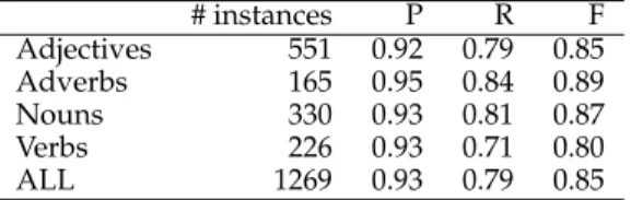
Findings: We find that the proposed measure of lexical contrast obtains high precision and large coverage, outperforming existing methods. Our method performs best on gradable pairs, antipodal pairs, and complementary pairs, but poorly on disjoint opposite pairs. Among different parts of speech, the method performs best on noun pairs, and relatively worse on verb pairs.

All of the data created and compiled as part of this research is summarized in Table 18 (Section 8), and is available for download.3

2. Related work

Charles and Miller (1989) proposed that opposites occur together in a sentence more often than chance. This is known as the co-occurrence hypothesis. Paradis et al. (2009) describe further experiments to show how canonical opposites tend to have high textual co-occurrence. Justeson and Katz (1991) gave evidence in support of the hypothesis using 35 prototypical opposites (from an original set of 39 opposites compiled by Deese (1965)) and also with an additional 22 frequent opposites. They also showed that opposites tend to occur in parallel syntactic constructions. All of these pairs were adjectives. Fellbaum (1995) conducted similar experiments on 47 noun, verb, adjective, and adverb pairs (noun–noun, noun–verb, noun–adjective, verb–adverb and so on) pertaining to 18 concepts (for example, lose(v)–gain(n) and loss(n)–gain(n), where lose(v) and loss(n) pertain to the concept of “failing to have/maintain”). However, non-opposite semantically related words also tend to occur together more often than chance. Thus, separating opposites from these other classes has proven to be difficult.

Some automatic methods of lexical contrast rely on lexical patterns in text. For example, Lin et al. (2003) used patterns such as “from X to Y ” and “either X or Y ” to separate opposites from distributionally similar pairs. They evaluated their method on 80 pairs of opposites and 80 pairs of synonyms taken from the Webster’s Collegiate

The-saurus (Kay 1988). The evaluation set of 160 word pairs was chosen such that it included

only high-frequency terms. This was necessary to increase the probability of finding sentences in a corpus where the target pair occurred in one of the chosen patterns. Lobanova et al. (2010) used a set of Dutch adjective seed pairs to learn lexical patterns commonly containing opposites. The patterns were in turn used to create a larger list of Dutch opposites. The method was evaluated by comparing entries to Dutch lexical resources and by asking human judges to determine whether an automatically found pair is indeed an opposite. Turney (2008) proposed a supervised method for identifying synonyms, opposites, hypernyms, and other lexical-semantic relations between word pairs. The approach learns patterns corresponding to different relations.

Harabagiu et al. (2006) detected contrasting word pairs for the purpose of identi-fying contradictions by using WordNet chains—synsets connected by the hypernymy– hyponymy links and exactly one antonymy link. Lucerto et al. (2002) proposed detecting contrasting word pairs using the number of tokens between two words in text and also

cue words such as but, from, and and. Unfortunately, they evaluated their method on only 18 word pairs. Neither Harabagiu et al. nor Lucerto et al. determined the degree of contrast between words and their methods have not been shown to have substantial coverage.

Schwab et al. (2002) created an oppositeness vector for a target word. The closer this vector is to the context vector of the other target word, the more opposite the two target words are. The oppositeness vectors were created by first manually identifying possible opposites and then generating suitable vectors for each using dictionary definitions. The approach was evaluated on only a handful of word pairs.

There is a large amount of work on sentiment analysis and opinion mining aimed at determining the polarity of words (Pang and Lee 2008). For example, Pang, Lee, and Vaithyanathan (2002) detected that adjectives such as dazzling, brilliant, and gripping cast their qualifying nouns positively whereas adjectives such as bad, cliched, and boring portray the noun negatively. Many of these gradable adjectives have opposites, but these approaches, with the exception of that of Hatzivassiloglou and McKeown (1997), did not attempt to determine pairs of positive and negative polarity words that are opposites. Hatzivassiloglou and McKeown (1997) proposed a supervised algorithm that uses word usage patterns to generate a graph with adjectives as nodes. An edge between two nodes indicates either that the two adjectives have the same or opposite polarity. A clustering algorithm then partitions the graph into two subgraphs such that the nodes in a subgraph have the same polarity. They used this method to create a lexicon of positive and negative words, and argued that the method could also be used to detect opposites.

3. The Heterogeneous Nature of Opposites

Opposites, unlike synonyms, can be of different kinds. Many different classifications have been proposed, one of which is given by Cruse (1986) (Chapters 9, 10, and 11). It consists of complementaries (open–shut, dead–alive), antonyms (long–short, slow–

fast) (further classified into polar, overlapping, and equipollent opposites), directional

opposites (up–down, north–south) (further classified into antipodals, counterparts, and reversives), relational opposites (husband–wife, predator–prey), indirect converses (give–

receive, buy–pay), congruence variants (huge–little, doctor–patient), and pseudo opposites

(black–white).

Various lexical relations have also received attention at the Educational Testing Services (ETS), as analogies and “most contrasting word” questions are part of the tests they conduct. They classify opposites into contradictories (alive–dead, masculine–

feminine), contraries (old–young, happy-sad), reverses (attack–defend, buy–sell),

direction-als (front–back, left–right), incompatibles (happy–morbid, frank–hypocritical), asymmetric contraries (hot–cool, dry–moist), pseudoopposites (popular–shy, right–bad), and defectives (default–payment, limp–walk) (Bejar, Chaffin, and Embretson 1991).

Keeping in mind the meanings and subtle distinctions between each of these kinds of opposites is not easy even if we provide extensive training to annotators. Since we crowdsource the annotations, and we know that Turkers prefer to spend their time do-ing the task (and makdo-ing money) rather than readdo-ing lengthy descriptions, we focused only on five kinds of opposites that we believed would be easiest to annotate, and which still captured a majority of the opposites:

r

Antipodals(top–bottom, start–finish): Antipodals are opposites in which

while the other term denotes the corresponding extreme in the other direction” (Cruse 1986).

r

Complementaries(open–shut, dead–alive): The essential characteristic of a

pair of complementaries is that “between them they exhaustively divide the conceptual domain into two mutually exclusive compartments, so that what does not fall into one of the compartments must necessarily fall into the other” (Cruse 1986).

r

Disjoint(hot–cold, like–dislike): Disjoint opposites are word pairs that

occupy non-overlapping regions in the semantic dimension such that there are regions not covered by either term. This set of opposites includes equipollent adjective pairs (for example, hot–cold) and stative verb pairs (for example, like–dislike). We refer the reader to Sections 9.4 and 9.7 of Cruse (1986) for details about these sub-kinds of opposites.

r

Gradable opposites(long–short, slow–fast): are adjective-pair or

adverb-pair opposites that are gradable, that is, “members of the pair denote degrees of some variable property such as length, speed, weight, accuracy, etc” (Cruse 1986).

r

Reversibles(rise–fall, enter–exit): Reversibles are opposite verb pairs such

that “if one member denotes a change from A to B, its reversive partner denotes a change from B to A” (Cruse 1986).

It should be noted that there is no agreed-upon number of kinds of opposites. Different researchers have proposed various classifications which overlap to a greater or lesser degree. It is possible that for a certain application or study one may be interested in a kind of opposite not listed above.

4. Crowdsourcing

We used the Amazon Mechanical Turk (AMT) service to obtain annotations for different kinds of opposites. We broke the task into small independently solvable units called

HITs (Human Intelligence Tasks) and uploaded them on the AMT website.4_{Each HIT had} a set of questions, all of which were to be answered by the same person (a Turker, in AMT parlance). We created HITs for word pairs, taken from WordNet, that we expected to have some degree of contrast in meaning.

In WordNet, words that are close in meaning are grouped together in a set called a

synset. If one of the words in a synset is an opposite of another word in a different synset,

then the two synsets are called head synsets and WordNet records the two words as direct

antonyms (Gross, Fischer, and Miller 1989)—WordNet regards the terms opposite and antonym as synonyms. Other word pairs across the two head synsets are called indirect antonyms. Since we follow Cruse’s definition of antonyms which requires antonyms to

be gradable adjectives, and since WordNet’s direct antonyms include noun, verb, and adverb pairs too, for the rest of the paper, we will refer to WordNet’s direct antonyms as direct opposites WordNet indirect antonyms as indirect opposites. We will refer to the union of both the direct and indirect opposites simply as WordNet opposites. Note that the WordNet opposites are highly contrasting term pairs.

Table 1

Target word pairs chosen for annotation. Each term was annotated about 8 times. part of speech # of word pairs

adverbs 185

adjectives 646

nouns 416

verbs 309

all 1556

We chose as target pairs all the direct or indirect opposites from WordNet that were also listed in the Macquarie Thesaurus. This condition was a mechanism to ignore less-frequent and obscure words, and apply our resources on words that are more common. Additionally, as we will describe ahead, we use the presence of the words in the thesaurus to help generate Question 1, which we use for quality control of the annotations. Table 1 gives a breakdown of the 1,556 pairs chosen by part of speech.

Since we do not have any control over the educational background of the anno-tators, we made efforts to phrase questions about the kinds of opposites in a simple and clear manner. Therefore we avoided definitions and long instructions in favor of examples and short questions. We believe this strategy is beneficial even in traditional annotation scenarios.

We created separate questionnaires (HITs) for adjectives, adverbs, nouns, and verbs. A complete example adjective HIT with directions and questions is shown in Figure 1. The adverb, noun, and verb questionnaires had similar questions, but were phrased slightly differently to accommodate differences in part of speech. These questionnaires are not shown here due to lack of space, but all four questionnaires are available for download.5_{The verb questionnaire had an additional question shown in Figure 2. Since} nouns and verbs are not considered gradable, the corresponding questionnaires did not have Q8 and Q9. We requested annotations from eight different Turkers for each HIT.

4.1 The Word Choice Question: Q1

Q1 is an automatically generated word choice question that has a clear correct answer. It helps identify outlier and malicious annotations. If this question is answered incorrectly, then we assume that the annotator does not know the meanings of the target words, and we ignore responses to the remaining questions. Further, as this question makes the annotator think about the meanings of the words and about the relationship between them, we believe it improves the responses for subsequent questions.

The options for Q1 were generated automatically. Each option is a set of four comma-separated words. The words in the answer are close in meaning to both of the target words. In order to create the answer option, we first generated a much larger source pool of all the words that were in the same thesaurus category as any of the two target words. (Words in the same category are closely related.) Words that had the same stem as either of the target words were discarded. For each of the remaining words, we

Word-pair: musical × dissonant

Q1.Which set of words is most related to the word pair musical:dissonant? r useless, surgery, ineffectual, institution

r sequence, episode, opus, composition r _{youngest, young, youthful, immature} r _{consequential, important, importance, heavy}

Q2.Do musical and dissonant have some contrast in meaning? r _yes r _no

For example, up–down, lukewarm–cold, teacher–student, attack–defend, all have at least some degree of contrast in meaning. On the other hand, clown–down, chilly–cold, teacher–doctor, and attack–rush DO NOT have contrasting meanings.

Q3.Some contrasting words are paired together so often that given one we naturally think of the other. If one of the words in such a pair were replaced with another word of almost the same meaning, it would sound odd. Are musical:dissonant such a pair?

r _yes r _no

Examples for “yes”: tall–short, attack–defend, honest–dishonest, happy–sad. Examples for “no”: tall–stocky, attack–protect, honest–liar, happy–morbid. Q5.Do musical and dissonant represent two ends or extremes?

r _yes r _no

Examples for “yes”: top–bottom, basement–attic, always–never, all–none, start–finish. Examples for “no”: hot–cold (boiling refers to more warmth than hot and freezing refers to less warmth than cold), teacher–student (there is no such thing as more or less teacher and more or less student), always–sometimes (never is fewer times than sometimes). Q6.If something is musical, would you assume it is not dissonant, and vice versa? In other words, would it be unusual for something to be both musical and dissonant?

r _yes r _no

Examples for “yes”: happy–sad, happy–morbid, vigilant–careless, slow–stationary. Examples for “no”: happy–calm, stationary–still, vigilant–careful, honest–truthful. Q7.If something or someone could possibly be either musical or dissonant, is it necessary that it must be either musical or dissonant? In other words, is it true that for things that can be musical or dissonant, there is no third possible state, except perhaps under highly unusual circumstances?

r _yes r _no

Examples for “yes”: partial–impartial, true–false, mortal–immortal.

Examples for “no”: hot–cold (an object can be at room temperature is neither hot nor cold), tall–short (a person can be of medium or average height).

Q8.In a typical situation, if two things or two people are musical, then can one be more musical than the other?

r yes r no

Examples for “yes”: quick, exhausting, loving, costly. Examples for “no”: dead, pregnant, unique, existent.

Q9.In a typical situation, if two things or two people are dissonant, can one be more dissonant than the other?

r _yes r _no

Examples for “yes”: quick, exhausting, loving, costly, beautiful. Examples for “no”: dead, pregnant, unique, existent, perfect, absolute.

Figure 1

Example HIT: Adjective pairs questionnaire.

Note: Perhaps “musical×dissonant” might be better written as “musical versus dissonant”, but we have kept “×” here to show the reader exactly what the Turkers were given.

Note: Q4 is not shown here, but can be seen in the online version of the questionnaire. It was an exploratory question, and it was not multiple choice. Q4’s responses have not been analyzed.

Word-pair: enabling×disabling

Q10.In a typical situation, do the sequence of actions disabling and then enabling bring someone or something back to the original state, AND do the sequence of actions enabling and disabling also bring someone or something back to the original state?

r

_{yes, both ways: the transition back to the initial state makes much sense in both sequences.}

r

_{yes, but only one way: the transition back to the original state makes much more sense one}

way, than the other way.

r

_{none of the above}

Examples for “yes, both ways”: enter–exit, dress–undress, tie–untie, appear–disappear. Examples for “yes, but only one way”: live–die, create–destroy, damage–repair, kill–resurrect. Examples for “none of the above”: leave–exit, teach–learn, attack–defend (attacking and then defending does not bring one back to the original state).

Figure 2

Additional question in the questionnaire for verbs.

Table 2

Number of word pairs and average number of annotations per word pair in the master set. part of # of average # of

speech word pairs annotations

adverbs 182 7.80

adjectives 631 8.32

nouns 405 8.44

verbs 288 7.58

all 1506 8.04

added their Lesk similarities with the two target words (Banerjee and Pedersen 2003). The four words with the highest sum were chosen to form the answer option.

The three distractor options were randomly selected from the pool of correct answers for all other word choice questions. Finally, the answer and distractor options were presented to the Turkers in random order.

4.2 Post-Processing

The response to a HIT by a Turker is called an assignment. We obtained about 12,448 assignments in all (1556 pairs×8 assignments each). About 7% of the adjective, adverb, and noun assignments and about 13% of the verb assignments had an incorrect answer to Q1. These assignments were discarded, leaving 1506 target pairs with three or more valid assignments. We will refer to this set of assignments as the master set, and all further analysis in this paper is based on this set. Table 2 gives a breakdown of the average number of annotations for each of the target pairs in the master set.

4.3 Prevalence of Different Kinds of Contrasting Pairs

For each question pertaining to every word pair in the master set, we determined the most frequent response by the annotators. Table 3 gives the percentage of word-pairs in the master set that received a most frequent response of “yes”. The first column in the table lists the question number followed by a brief description of question. (Note that the Turkers saw only the full forms of the questions, as shown in the example HIT.)

Table 3

Percentage of word pairs that received a response of “yes” for the questions in the questionnaire. ‘adj.’ stands for adjectives. ‘adv.’ stands for adverbs.

% of word pairs

Question answer adj. adv. nouns verbs

Q2. Do X and Y have some contrast? yes 99.5 96.8 97.6 99.3 Q3. Are X and Y opposites? yes 91.2 68.6 65.8 88.8 Q5. Are X and Y at two ends of a dimension? yes 81.8 73.5 81.1 94.4 Q6. Does X imply not Y? yes 98.3 92.3 89.4 97.5 Q7. Are X and Y mutually exhaustive? yes 85.1 69.7 74.1 89.5 Q8. Does X represent a point on some scale? yes 78.5 77.3 - -Q9. Does Y represent a point on some scale? yes 78.5 70.8 - -Q10. Does X undo Y OR does Y undo X? one way - - - 3.8 both ways - - - 90.9

Table 4

Percentage of WordNet source pairs that are contrasting, opposite, and “contrasting but not opposite”.

category basis adj. adv. nouns verbs

contrasting Q2 yes 99.5 96.8 97.6 99.3 opposites Q2 yes and Q3 yes 91.2 68.6 60.2 88.9 contrasting, but not opposite Q2 yes and Q3 no 8.2 28.2 37.4 10.4

Table 5

Percentage of contrasting word pairs belonging to various sub-types. The sub-type “reversives" applies only to verbs. The sub-type “gradable" applies only to adjectives and adverbs.

sub-type basis adv. adj. nouns verbs Antipodals Q2 yes, Q5 yes 82.3 75.9 82.5 95.1 Complementaries Q2 yes, Q7 yes 85.6 72.0 84.8 98.3 Disjoint Q2 yes, Q7 no 14.4 28.0 15.2 1.7 Gradable Q2 yes, Q8 yes, Q9 yes 69.6 66.4 - -Reversives Q2 yes, Q10 both ways - - - 91.6

Observe that most of the word pairs are considered to have at least some contrast in meaning. This is not surprising since the master set was constructed using words connected through WordNet’s antonymy relation.6Responses to Q3 show that not all contrasting pairs are considered opposite, and this is especially the case for adverb pairs and noun pairs. The rows in Table 4 show the percentage of words in the master set that are contrasting (row 1), opposite (row 2), and contrasting but not opposite (row 3).

Responses to Q5, Q6, Q7, Q8, and Q9 (Table 3) show the prevalence of different kinds of relations and properties of the target pairs.

Table 5 shows the percentage of contrasting word pairs that may be classified into the different types discussed in Section 3 earlier. Observe that rows for all categories other than the disjoints have percentages greater than 60%. This means that a number

6 All of the direct antonyms were marked as contrasting by the Turkers. Only a few indirect antonyms were marked as not contrasting.

Table 6

Breakdown of answer agreement by target-pair part of speech and question: For every target pair, a question is answered by about eight annotators. The majority response is chosen as the answer. The ratio of the size of the majority and the number of annotators is indicative of the amount of agreement. The table below shows the average percentage of this ratio.

question adj. adv. nouns verbs average

Q2. Do X and Y have some contrast? 90.7 92.1 92.0 94.7 92.4 Q3. Are X and Y opposites? 79.0 80.9 76.4 75.2 77.9 Q5. Are X and Y at two ends of a dimension? 70.3 66.5 73.0 78.6 72.1 Q6. Does X imply not Y? 89.0 90.2 81.8 88.4 87.4 Q7. Are X and Y mutually exhaustive? 70.4 69.2 78.2 88.3 76.5 average (Q2, Q3, Q5, Q6, and Q7) 82.3 79.8 80.3 85.0 81.3 Q8. Does X represent a point on some scale? 77.9 71.5 - - 74.7 Q9. Does Y represent a point on some scale? 75.2 72.0 - - 73.6 Q10. Does X undo Y OR does Y undo X? - - - 73.0 73.0 of contrasting word pairs can be classified into more than one kind. Complementaries are the most common kind in case of adverbs, nouns, and verbs, whereas antipodals are most common among adjectives. A majority of the adjective and adverb contrasting pairs are gradable, but more than 30% of the pairs are not. Most of the verb pairs are reversives (91.6%). Disjoint pairs are much less common than all the other categories considered, and they are most prominent among adjectives (28%), and least among verb pairs (1.7%).

4.4 Agreement

People do not always agree on linguistic classifications of terms, and one of the goals of this work was to determine how much people agree on properties relevant to different kinds of opposites. Table 6 lists the breakdown of agreement by target-pair part of speech and question, where agreement is the average percentage of the number of Turkers giving the most-frequent response to a question—the higher the number of Turkers that vote for the majority answer, the higher is the agreement.

Observe that agreement is highest when asked whether a word pair has some degree of contrast in meaning (Q2), and that there is a marked drop when asked if the two words are opposites (Q3). This is true for each of the parts of speech, although the drop is highest for verbs (94.7% to 75.2%).

For questions 5 through 9, we see varying degrees of agreement—Q6 obtaining the highest agreement and Q5 the lowest. There is marked difference across parts of speech for certain questions. For example, verbs are the easiest to identify (highest agreement for Q5, Q7, and Q8). For Q6, nouns have markedly lower agreement than all other parts of speech—not surprising considering that the set of disjoint opposites is traditionally associated with equipollent adjectives and stative verbs. Adverbs and adjectives have markedly lower agreement scores for Q7 than nouns and verbs.

5. Manifestation of highly contrasting word pairs in text

As pointed out earlier, there is work on a small set of opposites showing that opposites co-occur more often than chance (Charles and Miller 1989; Fellbaum 1995). Section 5.1 describes experiments on a larger scale to determine whether highly contrasting word pairs (including opposites) occur together more often than randomly chosen word

Table 7

Pointwise mutual information (PMI) of word pairs. High positive values imply a tendency to co-occur in text more often than random chance.

average PMI standard deviation high-contrast set 1.471 2.255 random pairs set 0.032 0.236 synonyms set 0.412 1.110

pairs of similar frequency. The section also compares co-occurrence associations with synonyms.

Research in distributional similarity has found that entries in distributional thesauri tend to also contain terms that are opposite in meaning (Lin 1998; Lin et al. 2003). Section 5.2 describes experiments to determine whether highly contrasting word pairs (including opposites) occur in similar contexts as often as randomly chosen pairs of words with similar frequencies, and whether highly contrasting words occur in similar contexts as often as synonyms.

5.1 Co-occurrence

In order to compare the tendencies of highly contrasting word pairs, synonyms, and random word pairs to co-occur in text, we created three sets of word pairs: the

high-contrast set, the synonyms set, and the control set of random word pairs. The high-high-contrast set

was created from a pool of direct and indirect opposites (nouns, verbs, and adjectives) from WordNet. We discarded pairs that did not meet the following conditions: (1) both members of the pair must be unigrams, (2) both members of the pair must occur in the

British National Corpus (BNC) (Burnard 2000), and (3) at least one member of the pair

must have a synonym in WordNet. A total of 1358 word pairs remained, and these form the high-contrast set.

Each of the pairs in the high-contrast set was used to create a synonym pair by choosing a WordNet synonym of exactly one member of the pair.7If a word has more than one synonym, then the most frequent synonym is chosen.8These 1358 word pairs form the synonyms set. Note that for each of the pairs in the high-contrast set, there is a corresponding pair in the synonyms set, such that the two pairs have a common term. For example, the pair agitation and calmness in the high-contrast set has a corresponding pair agitation and ferment in the synonyms set. We will refer to the common terms (agitation in the above example) as the focus words. Since we also wanted to compare occurrence statistics of the high-contrast set with the random pairs set, we created the control set of random pairs by taking each of the focus words and pairing them with another word in WordNet that has a frequency of occurrence in BNC closest to the term contrasting with the focus word. This is to ensure that members of the pairs across the high-contrast set and the control set have similar unigram frequencies.

We calculated the pointwise mutual information (PMI) (Church and Hanks 1990) for each of the word pairs in the high-contrast set, the random pairs set, and the synonyms set using unigram and co-occurrence frequencies in the BNC. If two words

7 If both members of a pair have WordNet synonyms, then one is chosen at random, and its synonym is taken.

occurred within a window of five adjacent words in a sentence, they were marked as co-occurring (same window as Church and Hanks (1990) used in their seminal work on word–word associations). Table 7 shows the average and standard deviation in each set. Observe that the high-contrast pairs have a much higher tendency to co-occur than the random pairs control set, and also the synonyms set. However, the high-contrast set has a large standard deviation. A two-sample t-test revealed that the high-contrast set is significantly different from the random set (p<_{0.05), and also that the high-contrast}

set is significantly different from the synonyms set (p<0.05).

However, on average the PMI between a focus word and its contrasting term was lower than the PMI between the focus word and 3559 other words in the BNC. These were often words related to the focus words, but nether contrasting nor synonymous. Thus, even though a high tendency to co-occur is a feature of highly contrasting pairs, it is not a sufficient condition for detecting them. We use PMI as part of our method for determining the degree of lexical contrast (described ahead in Section 6).

5.2 Distributional similarity

Charles and Miller (1989) proposed that in most contexts, opposites may be inter-changed. The meaning of the utterance will be inverted, of course, but the sentence will remain grammatical and linguistically plausible. This came to be known as the

substitutability hypothesis. However, their experiments did not support this claim. They

found that given a sentence with the target adjective removed, most people did not confound the missing word with its opposite. Justeson and Katz (1991) later showed that in sentences that contain both members of an adjectival opposite pair, the target adjectives do indeed occur in similar syntactic structures at the phrasal level. Jones et al. (2007) show how the tendency to appear in certain textual constructions such as “from X to Y” and “either X or Y” are indicative of prototypicalness of opposites. Thus, we can formulate the distributional hypothesis of highly contrasting pairs: highly contrasting pairs occur in similar contexts more often than non-contrasting word pairs.

We used the same sets of high-contrast pairs, synonyms, and random pairs de-scribed in the previous sub-section to gather empirical proof of the distributional hypothesis. We calculated the distributional similarity between each pair in the three sets using Lin’s (1998) measure. Table 8 shows the average and standard deviation in each set. Observe that the high-contrast set has a much higher average distributional similarity than the random pairs control set, and interestingly it is also higher than the synonyms set. Once again, the high-contrast set has a large standard deviation. A two-sample t-test revealed that the high-contrast set is significantly different from both the random set and the synonyms set with a confidence interval of 0.05. This demonstrates that relative to other word pairs, high-contrast pairs tend to occur in similar contexts. We also find that the synonyms set has a significantly higher distributional similarity than the random pairs set (p<0.05). This shows that near-synonymous word pairs

also occur in similar contexts (the distributional hypothesis of similarity). Further, a consequence of the large standard deviations in the cases of both high-contrast pairs and synonyms means that distributional similarity alone is not sufficient to determine whether two words are contrasting or synonymous. An automatic method for recog-nizing contrast will require additional cues. Our method uses PMI and other sources of information described in the next section.

Table 8

Distributional similarity of word pairs. The measure proposed in Lin (1998) was used. average distributional similarity standard deviation

opposites set 0.064 0.071

random pairs set 0.036 0.034

synonyms set 0.056 0.057

6. Computing Lexical Contrast

In this section, we recapitulate the automatic method for determining lexical contrast that we first proposed in Mohammad et al. (2008). Additional details are provided regarding the lexical resources used (Section 6.1) and the method itself (Section 6.2).

6.1 Lexical Resources

Our method makes use of a published thesaurus and co-occurrence information from text. Optionally, it can use opposites listed in WordNet if available. We briefly describe these resources here.

6.1.1 Published thesauri.Published thesauri, such as Roget’s and Macquarie, divide the vocabulary of a language into about a thousand categories. Words within a category are semantically related to each other, and they tend to pertain to a coarse concept. Each category is represented by a category number (unique ID) and a head word — a word that best represents the meanings of the words in the category. One may also find opposites in the same category, but this is rare. Words with more than one meaning may be found in more than one category; these represent its coarse senses.

Within a category, the words are grouped into finer units called paragraphs. Words in the same paragraph are closer in meaning than those in differing paragraphs. Each paragraph has a paragraph head — a word that best represents the meaning of the words in the paragraph. Words in a thesaurus paragraph belong to the same part of speech. A thesaurus category may have multiple paragraphs belonging to the same part of speech. For example, a category may have three noun paragraphs, four verb paragraphs, and one adjective paragraph. We will take advantage of the structure of the thesaurus in our approach.

6.1.2 WordNet.As mentioned earlier, WordNet encodes certain opposites. However, we found in our experiments (Section 7 below) that more than 90% of contrasting pairs included in Graduate Record Examination (GRE) “most contrasting word” questions are not encoded in WordNet.Also, neither WordNet nor any other manually-created repository of opposites provides the degree of contrast between word pairs. Neverthe-less, we investigate the usefulness of WordNet as a source of seed opposites for our approach.

6.2 Proposed Measure of Lexical Contrast

Our method for determining lexical contrast has two parts: (1) determining whether the target word pair is contrasting or not, and (2) determining the degree of contrast between the words.

Table 9

Fifteen affix patterns used to generate opposites. Here ‘X’ stands for any sequence of letters common to both words w1and w2.

affix pattern

pattern # word 1 word 2 # word pairs example pair 1 X antiX 41 clockwise–anticlockwise 2 X disX 379 interest–disinterest 3 X imX 193 possible–impossible 4 X inX 690 consistent–inconsistent 5 X malX 25 adroit–maladroit 6 X misX 142 fortune–misfortune 7 X nonX 72 aligned–nonaligned 8 X unX 833 biased–unbiased 9 lX illX 25 legal–illegal 10 rX irrX 48 regular–irregular 11 imX exX 35 implicit–explicit 12 inX exX 74 introvert–extrovert 13 upX downX 22 uphill–downhill 14 overX underX 52 overdone–underdone 15 Xless Xful 51 harmless–harmful

Total: 2682

6.2.1 Detecting whether a target word pair is contrasting.We use the contrast hypothe-sis to determine whether two words are contrasting. The hypothehypothe-sis is repeated below:

Contrast Hypothesis: If a pair of words, A and B, are contrasting, then there is a pair of opposites, C and D, such that A and C are strongly related and B and D are strongly related.

Even if a few exceptions to this hypothesis are found (we are not aware of any), the hypothesis would remain useful for practical applications. We first determine pairs of thesaurus categories that have at least one word in each category that are opposites of each other. We will refer to these categories as contrasting categories and the opposite connecting the two categories as the seed opposite. Since each thesaurus category is a collection of closely related terms, all of the word pairs across two contrasting categories satisfy the contrast hypothesis, and they are considered to be contrasting word pairs. Note also that words within a thesaurus category may belong to different parts of speech, and they may be related to the seed opposite word through any of the many possible semantic relations. Thus a small number of seed opposites can help identify a large number of contrasting word pairs.

We determine whether two categories are contrasting using the three methods described below, which may be used alone or in combination with each other:

Method 1: Using word pairs generated from affix patterns.

Opposites such as hot–cold and dark–light occur frequently in text, but in terms of type-pairs they are outnumbered by those created using affixes, such as un- (clear–unclear) and dis- (honest–dishonest). Further, this phenomenon is observed in most languages (Lyons 1977).

Table 9 lists fifteen affix patterns that tend to generate opposites in English. They were compiled by the first author by examining a small list of affixes for the English

language.9These patterns were applied to all words in the thesaurus that are at least three characters long. If the resulting term was also a valid word in the thesaurus, then the word-pair was added to the affix-generated seed set. These fifteen rules generated 2,682 word pairs when applied to the words in the Macquarie Thesaurus. Category pairs that had these opposites were marked as contrasting. Of course, not all of the word pairs generated through affixes are truly opposites, for example sect–insect and part–impart. For now, such pairs are sources of error in the system. Manual analysis of these 2,682 word pairs can help determine whether this error is large or small. (We have released the full set of word pairs.) However, evaluation results (Section 7) indicate that these seed pairs improve the overall accuracy of the system.

Figure 3 presents such an example pair. Observe that categories 360 and 361 have the words cover and uncover, respectively. Affix pattern 8 from Table 1 produces seed pair cover–uncover, and so the system concludes that the two categories have contrasting meaning. The contrast in meaning is especially strong for the paragraphs cover and

expose because words within these paragraphs are very close in meaning to cover and uncover, respectively. We will refer to such thesaurus paragraph pairs that have one

word each of a seed pair as prime contrasting paragraphs. We expect the words across prime contrasting paragraphs to have a high degree of antonymy (for example, mask and bare), whereas words across other contrasting category paragraphs may have a smaller degree of antonymy as the meaning of these words may diverge significantly from the meanings of the words in the prime contrasting paragraphs (for example,

white lie and disclosure).

Method 2: Using opposites from WordNet.

We compiled a list of 20,611 pairs that WordNet records as direct and indirect opposites. (Recall discussion in Section 4 about direct and indirect opposites.) A large number of these pairs include multiword expressions. Only 10,807 of the 20,611 pairs have both words in the Macquarie Thesaurus—the vocabulary used for our experiments. We will refer to them as the WordNet seed set. Category pairs that had these opposites were marked as contrasting.

Method 3: Using word pairs in adjacent thesaurus categories.

Most published thesauri, such as Roget’s, are organized such that categories correspond-ing to opposcorrespond-ing concepts are placed adjacent to each other. For example, in the Macquarie

Thesaurus: category 369 is about honesty and category 370 is about dishonesty; as shown

in Figure 3, category 360 is about hiding and category 361 is about revealing. There are a number of exceptions to this rule, and often a category may be contrasting in mean-ing to several other categories. However, since this was an easy-enough heuristic to implement, we investigated the usefulness of considering adjacent thesaurus categories as contrasting. We will refer to this as the adjacency heuristic. Note that this method of determining contrasting categories does not explicitly identify a seed opposite, but one can assume the head words of these category pairs as the seed opposites.

To determine how accurate the adjacency heuristic is, the first author manually inspected adjacent thesaurus categories in the Macquarie Thesaurus to determine which of them were indeed contrasting. Since a category, on average, has about a hundred words, the task was made less arduous by representing each category by just the first ten words listed in it. This way it took only about five hours to manually determine

3. verbs: hiding conceament covering screening

...

cover−up double blind smokescreen white lie

...

cover mask

...

curtain cushion 3. verbs: 1. nouns: Category number: 360 Category head: HIDING

2. nouns:

...

Category number: 361 Category head: REVEALING

1. nouns:

...

...

divulgement disclosure

...

uncover flush out

...

disinterment revealing exposure expose impartment unfoldment unveiling bare 2. nouns: Figure 3

Example contrasting category pair. The system identifies the pair to be contrasting through the affix-based seed pair cover–uncover. The paragraphs of cover and expose are referred to as prime contrasting paragraphs. Paragraph heads are shown in bold italic.

that 209 pairs of the 811 adjacent Macquarie category pairs were contrasting. Twice, it was found that category number X was contrasting not just to category number X+1 but also to category number X+2: category 40 (ARISTOCRACY) has a meaning that contrasts that of category 41 (MIDDLE CLASS) as well as category 42 (WORKING CLASS); category 542 (PAST) contrasts with category 543 (PRESENT) as well as category 544 (FUTURE). Both these X–(X+2) pairs are also added to the list of manually annotated contrasting categories.

6.2.2 Computing the degree of contrast between two words. Charles and Miller (1989) and Fellbaum (1995) argued that opposites tend to co-occur more often than random chance. Murphy and Andrew (1993) claimed that the greater-than-chance co-occurrence of opposites is because together they convey contrast well, which is rhetorically useful. We showed earlier in Section 5.1 that highly contrasting pairs (including opposites) co-occur more often than randomly chosen pairs. All of these support the degree of contrast hypothesis stated earlier in the introduction:

Degree of Contrast Hypothesis: If a pair of words, A and B, are contrasting, then their degree of contrast is proportional to their tendency to co-occur in a large corpus.

We used PMI to capture the tendency of word–word co-occurrence. We collected these co-occurrence statistics from the Google n-gram corpus (Brants and Franz 2006), which was created from a text collection of over 1 trillion words. Words that occurred within a window of 5 words were considered to be co-occurring.

1. nouns: Category number: 423 Category head: KINDNESS

1. nouns: Category number: 230 Category head: APATHY

kindness considerateness niceness goodness

...

2. adjectives: sympathetic consolatory caring involved

...

3. adverbs: benevolent beneficiently graciously kindheartedly

...

...

apathy acedia depression moppishness

...

2. nouns: nonchalance insouciance carelessness casualness 3. adjectives:

...

indifferent detached irresponsive uncaring

...

...

Figure 4

Example contrasting category pair that has Class II and Class III contrasting pairs. The system identifies the pair to be contrasting through the affix-based seed pair caring (second word in paragraph 2 or category 423) and uncaring (fourth word in paragraph 3 or category 230). The paragraphs of sympathetic and indifferent are therefore the prime contrasting paragraphs and so all word pairs that have one word each from these two paragraphs are Class II contrasting pairs. All other pairs formed by taking one word each from the two contrasting categories are the Class III contrasting pairs. Paragraph heads are shown in bold italic.

We expected that some features may be more accurate than others. If multiple features give evidence towards opposing information, then it is useful for the system to know which feature is more reliable. Therefore, we held out some data from the evaluation data described in Section 7.1 as the development set. Experiments on the development set showed that contrasting words may be placed in three bins corre-sponding to the amount of reliability of the source feature: high, medium, or acceptable.

r

High reliability (Class I):target words that belong to adjacent thesaurus

categories. For example, all the word pairs across categories 360 and 361, shown in Figure 3. Examples of class I contrasting word pairs from the development set include graceful–ungainly, fortunate–hapless, obese–slim, and effeminate–virile. (Note, there need not be any affix or WordNet seed pairs across adjacent thesaurus categories for these word pairs to be marked Class I.) As expected, if we use only those adjacent categories that were manually identified to be contrasting (as described in Section 6.2.1. method 3), then the system obtains even better results than those obtained using all adjacent thesaurus categories. (Experiments and results shown ahead in Section 7.1).

r

Medium reliability (Class II):target words that are not Class I contrasting

pairs, but belong to one paragraph each of a prime contrasting paragraph. For example, all the word pairs across the paragraphs of sympathetic and

the development set include altruism–avarice, miserly–munificent,

accept–repudiate, and improper–prim.

r

Acceptable reliability (Class III):target words that are not Class I or Class

II contrasting pairs, but occur across contrasting category pairs. For example, all word pairs across categories 423 and 230 except those that have one word each from the paragraphs of sympathetic and indifferent. See Figure 4. Examples of class III contrasting word pairs from the

development set include pandemonium–calm, probity–error, artifice–sincerity, and hapless–wealthy.

Even with access to very large textual datasets, there is always a long tail of words that occur so few times that there is not enough co-occurrence information for them. Thus we assume that all word pairs in Class I have a higher degree of contrast than all word pairs in Class II, and that all word pairs in Class II have a higher degree of contrast than the pairs in Class III. If two word pairs belong to the same class, then we calculate their tendency to co-occur with each other in text to determine which pair is more contrasting. All experiments in the evaluation section ahead follow this method.

6.2.3 Lexicon of contrasting word pairs.Using the method described in the previous sub-sections, we generated a lexicon of word pairs pertaining to Class I and Class II. The lexicon has 6.3 million contrasting word pairs, about 3.5 million of which belong to Class I and about 2.8 million to Class II. Class III pairs are even more numerous and given a word pair, our algorithm checked whether it is a class III pair, but we did not create a complete set of all Class III contrasting pairs. Class I and II lexicons are available for download and summarized in Table 18.

7. Evaluation

We evaluate our algorithm on two different tasks and four datasets. Section 7.1 describes experiments on solving existing GRE “choose the most contrasting word” questions (a recapitulation of the evaluation reported in Mohammad et al. (2008)). Section 7.2 describes experiments on solving newly created “choose the most contrasting word” questions specifically designed to determine performance on different kinds of oppo-sites. And lastly, Section 7.3 describes experiments on two different datasets where the goal is to identify whether a given word pair is synonymous or antonymous.

7.1 Solving GRE’s “choose the most contrasting word” questions

The Graduate Record Examination (GRE) is a test taken by thousands of North Ameri-can graduate school appliAmeri-cants. The test is administered by Educational Testing Service (ETS). The Verbal Reasoning section of GRE is designed to test verbal skills. Until August 2011, one of its sub-sections had a set of questions pertaining to word-pair contrast. Each question had a target word and four or five alternatives, or option words. The objective was to identify the alternative which was most contrasting with respect to the target. For example, consider:

Here the target word is adulterate. One of the alternatives provided is correct, which as a verb has a meaning that contrasts with that of adulterate; however, purify has a greater degree of contrast with adulterate than correct does and must be chosen in order for the instance to be marked as correctly answered. ETS referred to these questions as “antonym questions”, where the examinees had to “choose the word most nearly opposite” to the target. However, most of the target–answer pairs are not gradable adjectives, and since most of them are not opposites either, we will refer to these questions as “choose the most contrasting word” questions or contrast questions for short.

Evaluation on this dataset tests whether the automatic method is able to identify not just opposites but also those pairs that are not opposites but that have some degree of semantic contrast. Notably, for these questions, the method must be able to identify that one word pair has a higher degree of contrast than all others, even though that word pair may not necessarily be an opposite.

7.1.1 Data.A web search for large sets of contrast questions yielded two independent sets of questions designed to prepare students for the GRE. The first set consists of 162 questions. We used this set while we were developing our lexical contrast algorithm de-scribed in Section 4. Therefore, will refer to it as the development set. The development set helped determine which features of lexical contrast were more reliable than others. The second set has 1208 contrast questions. We discarded questions that had a multiword target or alternative. After removing duplicates we were left with 790 questions, which we used as the unseen test set. This dataset was used (and seen) only after our algorithm for determining lexical contrast was frozen.

Interestingly, the data contains many instances that have the same target word used in different senses. For example:

1. obdurate: a. meager b. unsusceptible c. right d. tender e. intelligent 2. obdurate: a. yielding b. motivated c. moribund d. azure e. hard 3. obdurate: a. transitory b. commensurate c. complaisant d. similar e. laconic In (1), obdurate is used in the sense ofHARDENED IN FEELINGSand is most contrasting with tender. In (2), it is used in the sense ofRESISTANT TO PERSUASION and is most contrasting with yielding. In (3), it is used in the sense of PERSISTENT and is most contrasting with transitory.

The datasets also contain questions in which one or more of the alternatives is a near-synonym of the target word. For example:

astute: a. shrewd b. foolish c. callow d. winning e. debating

Observe that shrewd is a near-synonym of astute. The word most contrasting with of

astute is foolish. A manual check of a randomly selected set of 100 test-set questions

revealed that, on average, one in four had a near-synonym as one of the alternatives.

7.1.2 Results. Table 10 presents results obtained on the development and test data using two baselines, a re-implementation of the method described in Lin et al. (2003), and variations of our method. Some of the results are for systems that refrain from attempting questions for which they do not have sufficient information. We therefore