Chapter 2
t (s) 0 50 100 150 " V || (V) -2 -1.8 -1.6 t (s) 0 50 100 150 " V ? (V) -2.2 -2 -1.8 t (s) 0 50 100 150 || " V|| 2 (V 2 ) #10-8 5 6 7 8 t (s) 0 50 100 150 I || 0.4534 0.4536 0.4538 0.454
Figure 2.1: ∆V and I vs t at U = 10−3m s−1, ω = 1571 rad s−1 and α = 0.3 %.
!M (rad/s) 0 0.2 0.4 0.6 0.8 1 " V || (V) #10-6 0 2 4 6 8 !M (rad/s) 0 0.2 0.4 0.6 0.8 1 " V ? (V) #10-6 0 2 4 6 ! M (rad/s) 0 0.2 0.4 0.6 0.8 1 || " V|| 2 -h || " V|| 2 i (V 2 ) #10 -10 0 2 4 6
Figure 2.2: FFT spectral density of ∆V vs ωM at U = 10−3m s−1, ω = 1571 rad s−1and
t (s) 0 50 100 150 " V || (V) #10-4 -4 -3 -2 -1 0 t (s) 0 50 100 150 " V ? (V) #10-4 -6 -4 -2 0 t (s) 0 50 100 150 || " V|| 2 (V 2 ) #10-7 0 1 2 3 t (s) 0 50 100 150 I || 0.438 0.4385 0.439 0.4395 0.44
Figure 2.3: ∆V and I vs t at U = 10−3m s−1, ω = 3142 rad s−1 and α = 0.3 %.
!M (rad/s) 0 0.2 0.4 0.6 0.8 1 " V || (V) #10-5 0 0.5 1 1.5 2 !M (rad/s) 0 0.2 0.4 0.6 0.8 1 " V ? (V) #10-5 0 0.5 1 1.5 2 ! M (rad/s) 0 0.2 0.4 0.6 0.8 1 || " V|| 2 -h || " V|| 2 i (V 2 ) #10 -9 0 1 2 3 4
Figure 2.4: FFT spectral density of ∆V vs ωM at U = 10−3m s−1, ω = 3142 rad s−1 and
t (s) 0 50 100 150 " V || (V) -2.6 -2.4 -2.2 t (s) 0 50 100 150 " V ? (V) -4 -3.5 t (s) 0 50 100 150 || " V|| 2 (V 2 ) #10-7 1.4 1.6 1.8 2 t (s) 0 50 100 150 I || 0.4236 0.4237 0.4238 0.4239
Figure 2.5: ∆V and I vs t at U = 10−3m s−1, ω = 4712 rad s−1 and α = 0.3 %.
!M (rad/s) 0 0.2 0.4 0.6 0.8 1 " V || (V) #10-5 0 1 2 3 !M (rad/s) 0 0.2 0.4 0.6 0.8 1 " V ? (V) #10-5 0 1 2 3 4 ! M (rad/s) 0 0.2 0.4 0.6 0.8 1 || " V|| 2 -h || " V|| 2 i (V 2 ) #10 -8 0 0.5 1 1.5
Figure 2.6: FFT spectral density of ∆V vs ωM at U = 10−3m s−1, ω = 4712 rad s−1and
t (s) 0 50 100 150 " V || (V) #10-4 -3 -2.5 -2 t (s) 0 50 100 150 " V ? (V) #10-4 -5 -4.5 -4 -3.5 -3 t (s) 0 50 100 150 || " V|| 2 (V 2 ) #10-7 1.5 2 2.5 3 t (s) 0 50 100 150 I || 0.4092 0.4093 0.4094 0.4095
Figure 2.7: ∆V and I vs t at U = 10−3m s−1, ω = 6283 rad s−1 and α = 0.3 %.
!M (rad/s) 0 0.2 0.4 0.6 0.8 1 " V || (V) #10-5 0 1 2 3 !M (rad/s) 0 0.2 0.4 0.6 0.8 1 " V ? (V) #10-5 0 2 4 6 ! M (rad/s) 0 0.2 0.4 0.6 0.8 1 || " V|| 2 -h || " V|| 2 i (V 2 ) #10 -8 0 1 2 3
Figure 2.8: FFT spectral density of ∆V vs ωM at U = 10−3m s−1, ω = 6283 rad s−1 and
t (s) 0 50 100 150 " V || (V) -3.5 -3 -2.5 t (s) 0 50 100 150 " V ? (V) -5.5 -5 -4.5 -4 t (s) 0 50 100 150 || " V|| 2 (V 2 ) #10-7 2 2.5 3 3.5 4 t (s) 0 50 100 150 I || 0.3942 0.3943 0.3944 0.3945 0.3946
Figure 2.9: ∆V and I vs t at U = 10−3m s−1, ω = 7854 rad s−1 and α = 0.3 %.
!M (rad/s) 0 0.2 0.4 0.6 0.8 1 " V || (V) #10-5 0 1 2 3 !M (rad/s) 0 0.2 0.4 0.6 0.8 1 " V ? (V) #10-5 0 2 4 6 8 ! M (rad/s) 0 0.2 0.4 0.6 0.8 1 || " V|| 2 -h || " V|| 2 i (V 2 ) #10 -8 0 2 4 6
Figure 2.10: FFT spectral density of ∆V vs ωM at U = 10−3m s−1, ω = 7854 rad s−1
t (s) 0 50 100 150 " V || (V) #10-4 -3.5 -3 -2.5 -2 t (s) 0 50 100 150 " V ? (V) #10-4 -7 -6 -5 -4 t (s) 0 50 100 150 || " V|| 2 (V 2 ) #10-7 2.5 3 3.5 4 4.5 t (s) 0 50 100 150 I || 0.3798 0.3799 0.3799 0.38 0.3800
Figure 2.11: ∆V and I vs t at U = 10−3m s−1, ω = 9425 rad s−1 and α = 0.3 %.
!M (rad/s) 0 0.2 0.4 0.6 0.8 1 " V || (V) #10-5 0 1 2 3 !M (rad/s) 0 0.2 0.4 0.6 0.8 1 " V ? (V) #10-4 0 0.5 1 ! M (rad/s) 0 0.2 0.4 0.6 0.8 1 || " V|| 2 -h || " V|| 2 i (V 2 ) #10 -8 0 2 4 6 8
Figure 2.12: FFT spectral density of ∆V vs ωM at U = 10−3m s−1, ω = 9425 rad s−1
t (s) 0 50 100 150 " V || (V) -3.5 -3 -2.5 t (s) 0 50 100 150 " V ? (V) -7 -6 -5 t (s) 0 50 100 150 || " V|| 2 (V 2 ) #10-7 3 4 5 6 t (s) 0 50 100 150 I || 0.3656 0.3657 0.3658 0.3659 0.366
Figure 2.13: ∆V and I vs t at U = 10−3m s−1, ω = 10 996 rad s−1 and α = 0.3 %.
!M (rad/s) 0 0.2 0.4 0.6 0.8 1 " V || (V) #10-5 0 1 2 3 4 !M (rad/s) 0 0.2 0.4 0.6 0.8 1 " V ? (V) #10-4 0 0.5 1 ! M (rad/s) 0 0.2 0.4 0.6 0.8 1 || " V|| 2 -h || " V|| 2 i (V 2 ) #10 -7 0 0.5 1
Figure 2.14: FFT spectral density of ∆V vs ωM at U = 10−3m s−1, ω = 10 996 rad s−1
t (s) 0 50 100 150 " V || (V) #10-4 -3.5 -3 -2.5 t (s) 0 50 100 150 " V ? (V) #10-4 -8 -7 -6 -5 -4 t (s) 0 50 100 150 || " V|| 2 (V 2 ) #10-7 3 4 5 6 t (s) 0 50 100 150 I || 0.3518 0.3519 0.352 0.3521
Figure 2.15: ∆V and I vs t at U = 10−3m s−1, ω = 12 566 rad s−1 and α = 0.3 %.
!M (rad/s) 0 0.2 0.4 0.6 0.8 1 " V || (V) #10-5 0 1 2 3 4 !M (rad/s) 0 0.2 0.4 0.6 0.8 1 " V ? (V) #10-4 0 0.5 1 1.5 ! M (rad/s) 0 0.2 0.4 0.6 0.8 1 || " V|| 2 -h || " V|| 2 i (V 2 ) #10 -7 0 0.5 1 1.5
Figure 2.16: FFT spectral density of ∆V vs ωM at U = 10−3m s−1, ω = 12 566 rad s−1
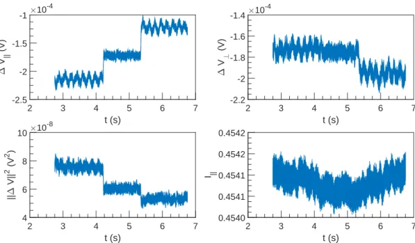
t (s) 2 3 4 5 6 7 " V || (V) -2.5 -2 -1.5 t (s) 2 3 4 5 6 7 " V ? (V) -2.2 -2 -1.8 -1.6 t (s) 2 3 4 5 6 7 || " V|| 2 (V 2 ) #10-8 4 6 8 10 t (s) 2 3 4 5 6 7 I || 0.4540 0.4541 0.4541 0.4542 0.4542
Figure 2.17: ∆V and I vs t at U = 0.1 m s−1, ω = 1571 rad s−1 and α = 0.3 %.
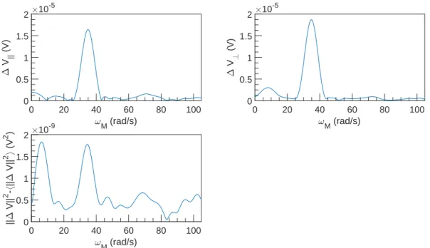
!M (rad/s) 0 20 40 60 80 100 " V || (V) #10-6 0 2 4 6 8 !M (rad/s) 0 20 40 60 80 100 " V ? (V) #10-6 0 2 4 6 ! M (rad/s) 0 20 40 60 80 100 || " V|| 2 -h || " V|| 2 i (V 2 ) #10 -9 0 0.5 1 1.5
Figure 2.18: FFT spectral density of ∆V vs ωM at U = 0.1 m s−1, ω = 1571 rad s−1 and
t (s) 2 3 4 5 6 7 " V || (V) #10-4 -6 -4 -2 0 t (s) 2 3 4 5 6 7 " V ? (V) #10-4 -6 -4 -2 0 t (s) 2 3 4 5 6 7 || " V|| 2 (V 2 ) #10-7 0 1 2 3 t (s) 2 3 4 5 6 7 I || 0.438 0.4385 0.439 0.4395 0.44
Figure 2.19: ∆V and I vs t at U = 0.1 m s−1, ω = 3142 rad s−1 and α = 0.3 %.
!M (rad/s) 0 20 40 60 80 100 " V || (V) #10-5 0 0.5 1 1.5 2 !M (rad/s) 0 20 40 60 80 100 " V ? (V) #10-5 0 0.5 1 1.5 2 ! M (rad/s) 0 20 40 60 80 100 || " V|| 2 -h || " V|| 2 i (V 2 ) #10 -9 0 0.5 1 1.5 2
Figure 2.20: FFT spectral density of ∆V vs ωM at U = 0.1 m s−1, ω = 3142 rad s−1 and
t (s) 3 4 5 6 7 8 " V || (V) -3 -2.5 -2 t (s) 3 4 5 6 7 8 " V ? (V) -4 -3.5 -3 t (s) 3 4 5 6 7 8 || " V|| 2 (V 2 ) #10-7 1.4 1.6 1.8 2 t (s) 3 4 5 6 7 8 I || 0.4241 0.4241 0.4241 0.4242 0.4242
Figure 2.21: ∆V and I vs t at U = 0.1 m s−1, ω = 4712 rad s−1 and α = 0.3 %.
!M (rad/s) 0 20 40 60 80 100 " V || (V) #10-5 0 1 2 3 !M (rad/s) 0 20 40 60 80 100 " V ? (V) #10-5 0 1 2 3 4 ! M (rad/s) 0 20 40 60 80 100 || " V|| 2 -h || " V|| 2 i (V 2 ) #10 -8 0 0.5 1 1.5
Figure 2.22: FFT spectral density of ∆V vs ωM at U = 0.1 m s−1, ω = 4712 rad s−1 and
t (s) 3 4 5 6 7 8 " V || (V) #10-4 -3.5 -3 -2.5 -2 -1.5 t (s) 3 4 5 6 7 8 " V ? (V) #10-4 -5 -4.5 -4 -3.5 -3 t (s) 3 4 5 6 7 8 || " V|| 2 (V 2 ) #10-7 1.5 2 2.5 3 t (s) 3 4 5 6 7 8 I || 0.4092 0.4093 0.4094 0.4095
Figure 2.23: ∆V and I vs t at U = 0.1 m s−1, ω = 6283 rad s−1 and α = 0.3 %.
!M (rad/s) 0 20 40 60 80 100 " V || (V) #10-5 0 1 2 3 !M (rad/s) 0 20 40 60 80 100 " V ? (V) #10-5 0 2 4 6 ! M (rad/s) 0 20 40 60 80 100 || " V|| 2 -h || " V|| 2 i (V 2 ) #10 -8 0 1 2 3
Figure 2.24: FFT spectral density of ∆V vs ωM at U = 0.1 m s−1, ω = 6283 rad s−1 and
t (s) 3 4 5 6 7 8 " V || (V) -3.5 -3 -2.5 t (s) 3 4 5 6 7 8 " V ? (V) -6 -5 -4 t (s) 3 4 5 6 7 8 || " V|| 2 (V 2 ) #10-7 2 2.5 3 3.5 4 t (s) 3 4 5 6 7 8 I || 0.3945 0.3945 0.3946 0.3946
Figure 2.25: ∆V and I vs t at U = 0.1 m s−1, ω = 7854 rad s−1 and α = 0.3 %.
!M (rad/s) 0 20 40 60 80 100 " V || (V) #10-5 0 1 2 3 !M (rad/s) 0 20 40 60 80 100 " V ? (V) #10-5 0 2 4 6 8 ! M (rad/s) 0 20 40 60 80 100 || " V|| 2 -h || " V|| 2 i (V 2 ) #10 -8 0 2 4 6
Figure 2.26: FFT spectral density of ∆V vs ωM at U = 0.1 m s−1, ω = 7854 rad s−1 and
t (s) 2 4 6 8 10 " V || (V) #10-4 -3.5 -3 -2.5 -2 t (s) 2 4 6 8 10 " V ? (V) #10-4 -7 -6 -5 -4 t (s) 2 4 6 8 10 || " V|| 2 (V 2 ) #10-7 2.5 3 3.5 4 4.5 t (s) 2 4 6 8 10 I || 0.3799 0.38 0.3801 0.3802
Figure 2.27: ∆V and I vs t at U = 0.1 m s−1, ω = 9425 rad s−1 and α = 0.3 %.
!M (rad/s) 0 20 40 60 80 100 " V || (V) #10-5 0 1 2 3 !M (rad/s) 0 20 40 60 80 100 " V ? (V) #10-5 0 2 4 6 8 ! M (rad/s) 0 20 40 60 80 100 || " V|| 2 -h || " V|| 2 i (V 2 ) #10 -8 0 2 4 6 8
Figure 2.28: FFT spectral density of ∆V vs ωM at U = 0.1 m s−1, ω = 9425 rad s−1 and
t (s) 3 4 5 6 7 8 " V || (V) -3.5 -3 -2.5 t (s) 3 4 5 6 7 8 " V ? (V) -7 -6 -5 t (s) 3 4 5 6 7 8 || " V|| 2 (V 2 ) #10-7 3 4 5 6 t (s) 3 4 5 6 7 8 I || 0.3656 0.3657 0.3658 0.3659 0.366
Figure 2.29: ∆V and I vs t at U = 0.1 m s−1, ω = 10 996 rad s−1 and α = 0.3 %.
!M (rad/s) 0 20 40 60 80 100 " V || (V) #10-5 0 1 2 3 !M (rad/s) 0 20 40 60 80 100 " V ? (V) #10-4 0 0.5 1 ! M (rad/s) 0 20 40 60 80 100 || " V|| 2 -h || " V|| 2 i (V 2 ) #10 -7 0 0.5 1
Figure 2.30: FFT spectral density of ∆V vs ωM at U = 0.1 m s−1, ω = 10 996 rad s−1
t (s) 4 6 8 10 12 " V || (V) #10-4 -3.5 -3 -2.5 -2 t (s) 4 6 8 10 12 " V ? (V) #10-4 -8 -7 -6 -5 -4 t (s) 4 6 8 10 12 || " V|| 2 (V 2 ) #10-7 3 4 5 6 t (s) 4 6 8 10 12 I || 0.3518 0.3519 0.352 0.3521 0.3522
Figure 2.31: ∆V and I vs t at U = 0.1 m s−1, ω = 12 566 rad s−1 and α = 0.3 %.
!M (rad/s) 0 20 40 60 80 100 " V || (V) #10-5 0 1 2 3 !M (rad/s) 0 20 40 60 80 100 " V ? (V) #10-4 0 0.5 1 1.5 ! M (rad/s) 0 20 40 60 80 100 || " V|| 2 -h || " V|| 2 i (V 2 ) #10 -7 0 0.5 1 1.5
Figure 2.32: FFT spectral density of ∆V vs ωM at U = 0.1 m s−1, ω = 12 566 rad s−1
t (s) 5 6 7 8 9 10 " V || (V) -2 -1 0 1 t (s) 5 6 7 8 9 10 " V ? (V) -2 -1 0 1 t (s) 5 6 7 8 9 10 || " V|| 2 (V 2 ) #10-6 0 1 2 3 4 t (s) 5 6 7 8 9 10 I || 0.44 0.45 0.46 0.47
Figure 2.33: ∆V and I vs t at U = 1 m s−1, ω = 1571 rad s−1 and α = 0.3 %.
!M (rad/s) 0 200 400 600 800 1000 " V || (V) #10-5 0 0.5 1 1.5 2 !M (rad/s) 0 200 400 600 800 1000 " V ? (V) #10-5 0 0.5 1 1.5 ! M (rad/s) 0 200 400 600 800 1000 || " V|| 2 -h || " V|| 2 i (V 2 ) #10 -8 0 1 2 3
Figure 2.34: FFT spectral density of ∆V vs ωM at U = 1 m s−1, ω = 1571 rad s−1 and
t (s) 2 3 4 5 6 " V || (V) #10-4 -10 -5 0 5 t (s) 2 3 4 5 6 " V ? (V) #10-4 -6 -4 -2 0 2 t (s) 2 3 4 5 6 || " V|| 2 (V 2 ) #10-7 0 2 4 6 t (s) 2 3 4 5 6 I || 0.437 0.438 0.439 0.44
Figure 2.35: ∆V and I vs t at U = 1 m s−1, ω = 3142 rad s−1 and α = 0.3 %.
!M (rad/s) 0 200 400 600 800 1000 " V || (V) #10-5 0 0.5 1 1.5 !M (rad/s) 0 200 400 600 800 1000 " V ? (V) #10-5 0 0.5 1 1.5 ! M (rad/s) 0 200 400 600 800 1000 || " V|| 2 -h || " V|| 2 i (V 2 ) #10 -8 0 0.5 1
Figure 2.36: FFT spectral density of ∆V vs ωM at U = 1 m s−1, ω = 3142 rad s−1 and
t (s) 4 5 6 7 8 " V || (V) -6 -4 -2 0 t (s) 4 5 6 7 8 " V ? (V) -6 -4 -2 t (s) 4 5 6 7 8 || " V|| 2 (V 2 ) #10-7 1 2 3 4 t (s) 4 5 6 7 8 I || 0.4236 0.4238 0.424 0.4242
Figure 2.37: ∆V and I vs t at U = 1 m s−1, ω = 4712 rad s−1 and α = 0.3 %.
!M (rad/s) 0 200 400 600 800 1000 " V || (V) #10-5 0 0.5 1 1.5 2 !M (rad/s) 0 200 400 600 800 1000 " V ? (V) #10-5 0 1 2 3 4 ! M (rad/s) 0 200 400 600 800 1000 || " V|| 2 -h || " V|| 2 i (V 2 ) #10 -9 0 2 4 6 8
Figure 2.38: FFT spectral density of ∆V vs ωM at U = 1 m s−1, ω = 4712 rad s−1 and
t (s) 3.5 4 4.5 5 5.5 6 " V || (V) #10-4 -6 -4 -2 0 2 t (s) 3.5 4 4.5 5 5.5 6 " V ? (V) #10-4 -6 -5 -4 -3 -2 t (s) 3.5 4 4.5 5 5.5 6 || " V|| 2 (V 2 ) #10-7 1 2 3 4 t (s) 3.5 4 4.5 5 5.5 6 I || 0.4091 0.4091 0.4092 0.4092 0.4093
Figure 2.39: ∆V and I vs t at U = 1 m s−1, ω = 6283 rad s−1 and α = 0.3 %.
!M (rad/s) 0 200 400 600 800 1000 " V || (V) #10-5 0 1 2 3 !M (rad/s) 0 200 400 600 800 1000 " V ? (V) #10-5 0 2 4 6 ! M (rad/s) 0 200 400 600 800 1000 || " V|| 2 -h || " V|| 2 i (V 2 ) #10 -9 0 2 4 6 8
Figure 2.40: FFT spectral density of ∆V vs ωM at U = 1 m s−1, ω = 6283 rad s−1 and
t (s) 4 4.5 5 5.5 6 6.5 " V || (V) -6 -4 -2 t (s) 4 4.5 5 5.5 6 6.5 " V ? (V) -8 -6 -4 t (s) 4 4.5 5 5.5 6 6.5 || " V|| 2 (V 2 ) #10-7 2 3 4 5 t (s) 4 4.5 5 5.5 6 6.5 I || 0.3944 0.3944 0.3944 0.3945 0.3945
Figure 2.41: ∆V and I vs t at U = 1 m s−1, ω = 7854 rad s−1 and α = 0.3 %.
!M (rad/s) 0 200 400 600 800 1000 " V || (V) #10-5 0 1 2 3 !M (rad/s) 0 200 400 600 800 1000 " V ? (V) #10-5 0 2 4 6 ! M (rad/s) 0 200 400 600 800 1000 || " V|| 2 -h || " V|| 2 i (V 2 ) #10 -8 0 0.5 1 1.5 2
Figure 2.42: FFT spectral density of ∆V vs ωM at U = 1 m s−1, ω = 7854 rad s−1 and
t (s) 3 4 5 6 " V || (V) #10-4 -6 -4 -2 0 t (s) 3 4 5 6 " V ? (V) #10-4 -8 -6 -4 -2 t (s) 3 4 5 6 || " V|| 2 (V 2 ) #10-7 2 3 4 5 6 t (s) 3 4 5 6 I || 0.3798 0.3799 0.38 0.3801
Figure 2.43: ∆V and I vs t at U = 1 m s−1, ω = 9425 rad s−1 and α = 0.3 %.
!M (rad/s) 0 200 400 600 800 1000 " V || (V) #10-5 0 1 2 3 !M (rad/s) 0 200 400 600 800 1000 " V ? (V) #10-5 0 2 4 6 8 ! M (rad/s) 0 200 400 600 800 1000 || " V|| 2 -h || " V|| 2 i (V 2 ) #10 -8 0 1 2 3 4
Figure 2.44: FFT spectral density of ∆V vs ωM at U = 1 m s−1, ω = 9425 rad s−1 and
t (s) 2 3 4 5 6 " V || (V) -5 -4 -3 -2 t (s) 2 3 4 5 6 " V ? (V) -8 -6 -4 t (s) 2 3 4 5 6 || " V|| 2 (V 2 ) #10-7 2 3 4 5 6 t (s) 2 3 4 5 6 I || 0.3656 0.3657 0.3658 0.3659
Figure 2.45: ∆V and I vs t at U = 1 m s−1, ω = 10 996 rad s−1 and α = 0.3 %.
!M (rad/s) 0 200 400 600 800 1000 " V || (V) #10-5 0 1 2 3 !M (rad/s) 0 200 400 600 800 1000 " V ? (V) #10-4 0 0.5 1 ! M (rad/s) 0 200 400 600 800 1000 || " V|| 2 -h || " V|| 2 i (V 2 ) #10 -8 0 2 4 6
Figure 2.46: FFT spectral density of ∆V vs ωM at U = 1 m s−1, ω = 10 996 rad s−1 and
t (s) 4 5 6 7 8 " V || (V) #10-4 -5 -4 -3 -2 -1 t (s) 4 5 6 7 8 " V ? (V) #10-4 -10 -8 -6 -4 -2 t (s) 4 5 6 7 8 || " V|| 2 (V 2 ) #10-7 3 4 5 6 7 t (s) 4 5 6 7 8 I || 0.3518 0.3519 0.352 0.3521 0.3522
Figure 2.47: ∆V and I vs t at U = 1 m s−1, ω = 12 566 rad s−1 and α = 0.3 %.
!M (rad/s) 0 200 400 600 800 1000 " V || (V) #10-5 0 1 2 3 !M (rad/s) 0 200 400 600 800 1000 " V ? (V) #10-4 0 0.5 1 ! M (rad/s) 0 200 400 600 800 1000 || " V|| 2 -h || " V|| 2 i (V 2 ) #10 -8 0 2 4 6 8
Figure 2.48: FFT spectral density of ∆V vs ωM at U = 1 m s−1, ω = 12 566 rad s−1 and
t (s) 0 50 100 150 " V || (V) -4 -3 -2 -1 t (s) 0 50 100 150 " V ? (V) -6 -4 -2 t (s) 0 50 100 150 || " V|| 2 (V 2 ) #10-7 0 1 2 3 t (s) 0 50 100 150 I || 0.438 0.4385 0.439 0.4395 0.44
Figure 2.49: ∆V and I vs t at U = 10−3m s−1, ω = 3142 rad s−1 and α = 0.3 %.
!M (rad/s) 0 0.2 0.4 0.6 0.8 1 " V || (V) #10-5 0 0.5 1 1.5 2 !M (rad/s) 0 0.2 0.4 0.6 0.8 1 " V ? (V) #10-5 0 0.5 1 1.5 2 ! M (rad/s) 0 0.2 0.4 0.6 0.8 1 || " V|| 2 -h || " V|| 2 i (V 2 ) #10 -9 0 1 2 3 4
Figure 2.50: FFT spectral density of ∆V vs ωM at U = 10−3m s−1, ω = 3142 rad s−1
t (s) 0 50 100 150 " V || (V) #10-4 -3 -2.5 -2 t (s) 0 50 100 150 " V ? (V) #10-4 -5 -4.5 -4 -3.5 -3 t (s) 0 50 100 150 || " V|| 2 (V 2 ) #10-7 1.5 2 2.5 3 t (s) 0 50 100 150 I || 0.4092 0.4093 0.4094 0.4095
Figure 2.51: ∆V and I vs t at U = 10−3m s−1, ω = 6283 rad s−1 and α = 0.3 %.
!M (rad/s) 0 0.2 0.4 0.6 0.8 1 " V || (V) #10-5 0 1 2 3 !M (rad/s) 0 0.2 0.4 0.6 0.8 1 " V ? (V) #10-5 0 2 4 6 ! M (rad/s) 0 0.2 0.4 0.6 0.8 1 || " V|| 2 -h || " V|| 2 i (V 2 ) #10 -8 0 1 2 3
Figure 2.52: FFT spectral density of ∆V vs ωM at U = 10−3m s−1, ω = 6283 rad s−1
t (s) 0 50 100 150 " V || (V) -4 -3 -2 -1 t (s) 0 50 100 150 " V ? (V) -6 -4 -2 t (s) 0 50 100 150 || " V|| 2 (V 2 ) #10-7 0 1 2 3 t (s) 0 50 100 150 I || 0.437 0.438 0.439 0.44
Figure 2.53: ∆V and I vs t at U = 3 × 10⁻³m s−1, ω = 3142 rad s−1 and α = 0.3 %.
!M (rad/s) 0 1 2 3 " V || (V) #10-5 0 0.5 1 1.5 2 !M (rad/s) 0 1 2 3 " V ? (V) #10-5 0 0.5 1 1.5 2 ! M (rad/s) 0 1 2 3 || " V|| 2 -h || " V|| 2 i (V 2 ) #10 -9 0 1 2 3 4
Figure 2.54: FFT spectral density of ∆V vs ωM at U = 3 × 10⁻³m s−1, ω = 3142 rad s−1
t (s) 0 50 100 150 " V || (V) #10-4 -3 -2.5 -2 t (s) 0 50 100 150 " V ? (V) #10-4 -5 -4.5 -4 -3.5 -3 t (s) 0 50 100 150 || " V|| 2 (V 2 ) #10-7 1.5 2 2.5 3 t (s) 0 50 100 150 I || 0.4091 0.4092 0.4093 0.4094
Figure 2.55: ∆V and I vs t at U = 3 × 10⁻³m s−1, ω = 6283 rad s−1 and α = 0.3 %.
!M (rad/s) 0 1 2 3 " V || (V) #10-5 0 1 2 3 !M (rad/s) 0 1 2 3 " V ? (V) #10-5 0 2 4 6 ! M (rad/s) 0 1 2 3 || " V|| 2 -h || " V|| 2 i (V 2 ) #10 -8 0 1 2 3
Figure 2.56: FFT spectral density of ∆V vs ωM at U = 3 × 10⁻³m s−1, ω = 6283 rad s−1
t (s) 0 10 20 30 40 " V || (V) -4 -3 -2 -1 t (s) 0 10 20 30 40 " V ? (V) -6 -4 -2 t (s) 0 10 20 30 40 || " V|| 2 (V 2 ) #10-7 0 1 2 3 t (s) 0 10 20 30 40 I || 0.437 0.438 0.439 0.44
Figure 2.57: ∆V and I vs t at U = 10−2m s−1, ω = 3142 rad s−1 and α = 0.3 %.
!M (rad/s) 0 2 4 6 8 10 " V || (V) #10-5 0 0.5 1 1.5 2 !M (rad/s) 0 2 4 6 8 10 " V ? (V) #10-5 0 0.5 1 1.5 2 ! M (rad/s) 0 2 4 6 8 10 || " V|| 2 -h || " V|| 2 i (V 2 ) #10 -9 0 1 2 3 4
Figure 2.58: FFT spectral density of ∆V vs ωM at U = 10−2m s−1, ω = 3142 rad s−1
t (s) 0 10 20 30 40 " V || (V) #10-4 -3 -2.5 -2 t (s) 0 10 20 30 40 " V ? (V) #10-4 -5 -4.5 -4 -3.5 -3 t (s) 0 10 20 30 40 || " V|| 2 (V 2 ) #10-7 1.5 2 2.5 3 t (s) 0 10 20 30 40 I || 0.4091 0.4092 0.4093 0.4094
Figure 2.59: ∆V and I vs t at U = 10−2m s−1, ω = 6283 rad s−1 and α = 0.3 %.
!M (rad/s) 0 2 4 6 8 10 " V || (V) #10-5 0 1 2 3 !M (rad/s) 0 2 4 6 8 10 " V ? (V) #10-5 0 2 4 6 ! M (rad/s) 0 2 4 6 8 10 || " V|| 2 -h || " V|| 2 i (V 2 ) #10 -8 0 1 2 3
Figure 2.60: FFT spectral density of ∆V vs ωM at U = 10−2m s−1, ω = 6283 rad s−1
t (s) 5 10 15 20 " V || (V) -4 -3 -2 -1 t (s) 5 10 15 20 " V ? (V) -6 -4 -2 t (s) 5 10 15 20 || " V|| 2 (V 2 ) #10-7 0 1 2 3 t (s) 5 10 15 20 I || 0.438 0.4385 0.439 0.4395 0.44
Figure 2.61: ∆V and I vs t at U = 3 × 10⁻²m s−1, ω = 3142 rad s−1 and α = 0.3 %.
!M (rad/s) 0 10 20 30 " V || (V) #10-5 0 0.5 1 1.5 2 !M (rad/s) 0 10 20 30 " V ? (V) #10-5 0 0.5 1 1.5 2 ! M (rad/s) 0 10 20 30 || " V|| 2 -h || " V|| 2 i (V 2 ) #10 -9 0 1 2 3
Figure 2.62: FFT spectral density of ∆V vs ωM at U = 3 × 10⁻²m s−1, ω = 3142 rad s−1
t (s) 0 5 10 15 20 " V || (V) #10-4 -3.5 -3 -2.5 -2 t (s) 0 5 10 15 20 " V ? (V) #10-4 -5 -4.5 -4 -3.5 -3 t (s) 0 5 10 15 20 || " V|| 2 (V 2 ) #10-7 1.5 2 2.5 3 t (s) 0 5 10 15 20 I || 0.4091 0.4092 0.4093 0.4094
Figure 2.63: ∆V and I vs t at U = 3 × 10⁻²m s−1, ω = 6283 rad s−1 and α = 0.3 %.
!M (rad/s) 0 10 20 30 " V || (V) #10-5 0 1 2 3 !M (rad/s) 0 10 20 30 " V ? (V) #10-5 0 2 4 6 ! M (rad/s) 0 10 20 30 || " V|| 2 -h || " V|| 2 i (V 2 ) #10 -8 0 1 2 3
Figure 2.64: FFT spectral density of ∆V vs ωM at U = 3 × 10⁻²m s−1, ω = 6283 rad s−1
t (s) 2 3 4 5 6 7 " V || (V) -6 -4 -2 t (s) 2 3 4 5 6 7 " V ? (V) -6 -4 -2 t (s) 2 3 4 5 6 7 || " V|| 2 (V 2 ) #10-7 0 1 2 3 t (s) 2 3 4 5 6 7 I || 0.438 0.4385 0.439 0.4395 0.44
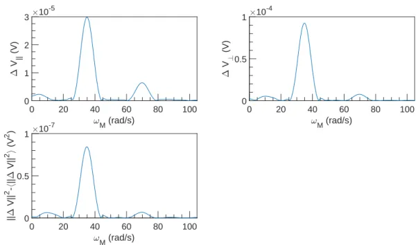
Figure 2.65: ∆V and I vs t at U = 0.1 m s−1, ω = 3142 rad s−1 and α = 0.3 %.
!M (rad/s) 0 20 40 60 80 100 " V || (V) #10-5 0 0.5 1 1.5 2 !M (rad/s) 0 20 40 60 80 100 " V ? (V) #10-5 0 0.5 1 1.5 2 ! M (rad/s) 0 20 40 60 80 100 || " V|| 2 -h || " V|| 2 i (V 2 ) #10 -9 0 0.5 1 1.5 2
Figure 2.66: FFT spectral density of ∆V vs ωM at U = 0.1 m s−1, ω = 3142 rad s−1 and
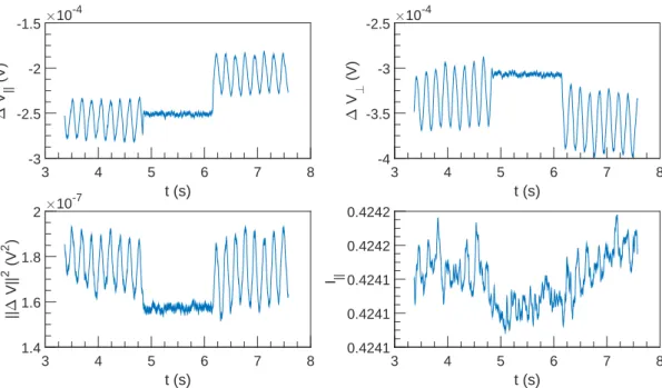
t (s) 3 4 5 6 7 8 " V || (V) #10-4 -3.5 -3 -2.5 -2 -1.5 t (s) 3 4 5 6 7 8 " V ? (V) #10-4 -5 -4.5 -4 -3.5 -3 t (s) 3 4 5 6 7 8 || " V|| 2 (V 2 ) #10-7 1.5 2 2.5 3 t (s) 3 4 5 6 7 8 I || 0.4092 0.4093 0.4094 0.4095
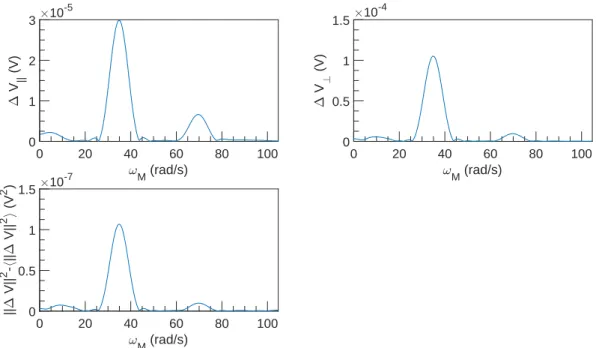
Figure 2.67: ∆V and I vs t at U = 0.1 m s−1, ω = 6283 rad s−1 and α = 0.3 %.
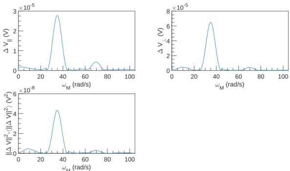
!M (rad/s) 0 20 40 60 80 100 " V || (V) #10-5 0 1 2 3 !M (rad/s) 0 20 40 60 80 100 " V ? (V) #10-5 0 2 4 6 ! M (rad/s) 0 20 40 60 80 100 || " V|| 2 -h || " V|| 2 i (V 2 ) #10 -8 0 1 2 3
Figure 2.68: FFT spectral density of ∆V vs ωM at U = 0.1 m s−1, ω = 6283 rad s−1 and
t (s) 3 4 5 6 7 " V || (V) -6 -4 -2 0 t (s) 3 4 5 6 7 " V ? (V) -6 -4 -2 t (s) 3 4 5 6 7 || " V|| 2 (V 2 ) #10-7 0 1 2 3 t (s) 3 4 5 6 7 I || 0.438 0.4385 0.439 0.4395 0.44
Figure 2.69: ∆V and I vs t at U = 0.25 m s−1, ω = 3142 rad s−1 and α = 0.3 %.
!M (rad/s) 0 50 100 150 200 250 " V || (V) #10-5 0 0.5 1 1.5 2 !M (rad/s) 0 50 100 150 200 250 " V ? (V) #10-5 0 0.5 1 1.5 2 ! M (rad/s) 0 50 100 150 200 250 || " V|| 2 -h || " V|| 2 i (V 2 ) #10 -9 0 0.5 1 1.5
Figure 2.70: FFT spectral density of ∆V vs ωM at U = 0.25 m s−1, ω = 3142 rad s−1
t (s) 2 3 4 5 " V || (V) #10-4 -3.5 -3 -2.5 -2 -1.5 t (s) 2 3 4 5 " V ? (V) #10-4 -6 -5 -4 -3 t (s) 2 3 4 5 || " V|| 2 (V 2 ) #10-7 1.5 2 2.5 3 t (s) 2 3 4 5 I || 0.4091 0.4092 0.4092 0.4093 0.4093
Figure 2.71: ∆V and I vs t at U = 0.25 m s−1, ω = 6283 rad s−1 and α = 0.3 %.
!M (rad/s) 0 50 100 150 200 250 " V || (V) #10-5 0 1 2 3 !M (rad/s) 0 50 100 150 200 250 " V ? (V) #10-5 0 2 4 6 ! M (rad/s) 0 50 100 150 200 250 || " V|| 2 -h || " V|| 2 i (V 2 ) #10 -8 0 1 2 3
Figure 2.72: FFT spectral density of ∆V vs ωM at U = 0.25 m s−1, ω = 6283 rad s−1
t (s) 2 3 4 5 6 " V || (V) -6 -4 -2 0 t (s) 2 3 4 5 6 " V ? (V) -6 -4 -2 t (s) 2 3 4 5 6 || " V|| 2 (V 2 ) #10-7 0 1 2 3 4 t (s) 2 3 4 5 6 I || 0.438 0.4385 0.439 0.4395 0.44
Figure 2.73: ∆V and I vs t at U = 0.5 m s−1, ω = 3142 rad s−1 and α = 0.3 %.
!M (rad/s) 0 100 200 300 400 500 " V || (V) #10-5 0 0.5 1 1.5 !M (rad/s) 0 100 200 300 400 500 " V ? (V) #10-5 0 0.5 1 1.5 2 ! M (rad/s) 0 100 200 300 400 500 || " V|| 2 -h || " V|| 2 i (V 2 ) #10 -9 0 1 2 3 4
Figure 2.74: FFT spectral density of ∆V vs ωM at U = 0.5 m s−1, ω = 3142 rad s−1 and
t (s) 3 4 5 6 7 " V || (V) #10-4 -6 -4 -2 0 t (s) 3 4 5 6 7 " V ? (V) #10-4 -6 -5 -4 -3 -2 t (s) 3 4 5 6 7 || " V|| 2 (V 2 ) #10-7 1.5 2 2.5 3 3.5 t (s) 3 4 5 6 7 I || 0.4091 0.4091 0.4092 0.4092 0.4093
Figure 2.75: ∆V and I vs t at U = 0.5 m s−1, ω = 6283 rad s−1 and α = 0.3 %.
!M (rad/s) 0 100 200 300 400 500 " V || (V) #10-5 0 1 2 3 !M (rad/s) 0 100 200 300 400 500 " V ? (V) #10-5 0 2 4 6 ! M (rad/s) 0 100 200 300 400 500 || " V|| 2 -h || " V|| 2 i (V 2 ) #10 -8 0 0.5 1 1.5 2
Figure 2.76: FFT spectral density of ∆V vs ωM at U = 0.5 m s−1, ω = 6283 rad s−1 and
t (s) 2 3 4 5 " V || (V) -10 -5 0 t (s) 2 3 4 5 " V ? (V) -6 -4 -2 0 t (s) 2 3 4 5 || " V|| 2 (V 2 ) #10-7 0 1 2 3 4 t (s) 2 3 4 5 I || 0.437 0.438 0.439 0.44
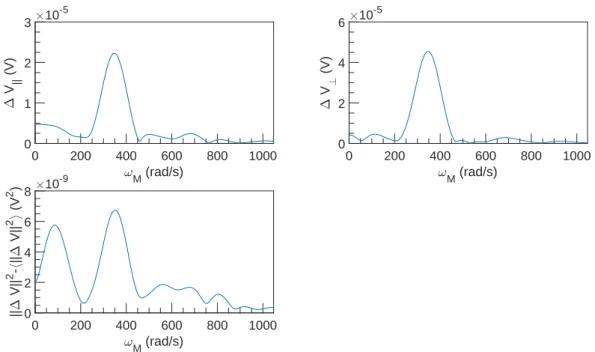
Figure 2.77: ∆V and I vs t at U = 0.75 m s−1, ω = 3142 rad s−1 and α = 0.3 %.
!M (rad/s) 0 200 400 600 " V || (V) #10-5 0 0.5 1 1.5 !M (rad/s) 0 200 400 600 " V ? (V) #10-5 0 0.5 1 1.5 2 ! M (rad/s) 0 200 400 600 || " V|| 2 -h || " V|| 2 i (V 2 ) #10 -8 0 0.5 1
Figure 2.78: FFT spectral density of ∆V vs ωM at U = 0.75 m s−1, ω = 3142 rad s−1
t (s) 4 5 6 7 8 " V || (V) #10-4 -6 -4 -2 0 t (s) 4 5 6 7 8 " V ? (V) #10-4 -6 -5 -4 -3 -2 t (s) 4 5 6 7 8 || " V|| 2 (V 2 ) #10-7 1.5 2 2.5 3 3.5 t (s) 4 5 6 7 8 I || 0.409 0.4091 0.4092 0.4093
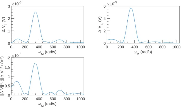
Figure 2.79: ∆V and I vs t at U = 0.75 m s−1, ω = 6283 rad s−1 and α = 0.3 %.
!M (rad/s) 0 200 400 600 " V || (V) #10-5 0 1 2 3 !M (rad/s) 0 200 400 600 " V ? (V) #10-5 0 2 4 6 ! M (rad/s) 0 200 400 600 || " V|| 2 -h || " V|| 2 i (V 2 ) #10 -8 0 0.5 1 1.5
Figure 2.80: FFT spectral density of ∆V vs ωM at U = 0.75 m s−1, ω = 6283 rad s−1
t (s) 2 3 4 5 6 " V || (V) -10 -5 0 t (s) 2 3 4 5 6 " V ? (V) -6 -4 -2 0 t (s) 2 3 4 5 6 || " V|| 2 (V 2 ) #10-7 0 2 4 6 t (s) 2 3 4 5 6 I || 0.437 0.438 0.439 0.44
Figure 2.81: ∆V and I vs t at U = 1 m s−1, ω = 3142 rad s−1 and α = 0.3 %.
!M (rad/s) 0 200 400 600 800 1000 " V || (V) #10-5 0 0.5 1 1.5 !M (rad/s) 0 200 400 600 800 1000 " V ? (V) #10-5 0 0.5 1 1.5 ! M (rad/s) 0 200 400 600 800 1000 || " V|| 2 -h || " V|| 2 i (V 2 ) #10 -8 0 0.5 1
Figure 2.82: FFT spectral density of ∆V vs ωM at U = 1 m s−1, ω = 3142 rad s−1 and
t (s) 3.5 4 4.5 5 5.5 6 " V || (V) #10-4 -6 -4 -2 0 2 t (s) 3.5 4 4.5 5 5.5 6 " V ? (V) #10-4 -6 -5 -4 -3 -2 t (s) 3.5 4 4.5 5 5.5 6 || " V|| 2 (V 2 ) #10-7 1 2 3 4 t (s) 3.5 4 4.5 5 5.5 6 I || 0.4091 0.4091 0.4092 0.4092 0.4093
Figure 2.83: ∆V and I vs t at U = 1 m s−1, ω = 6283 rad s−1 and α = 0.3 %.
!M (rad/s) 0 200 400 600 800 1000 " V || (V) #10-5 0 1 2 3 !M (rad/s) 0 200 400 600 800 1000 " V ? (V) #10-5 0 2 4 6 ! M (rad/s) 0 200 400 600 800 1000 || " V|| 2 -h || " V|| 2 i (V 2 ) #10 -9 0 2 4 6 8
Figure 2.84: FFT spectral density of ∆V vs ωM at U = 1 m s−1, ω = 6283 rad s−1 and