Publisher’s version / Version de l'éditeur:
Vous avez des questions? Nous pouvons vous aider. Pour communiquer directement avec un auteur, consultez la première page de la revue dans laquelle son article a été publié afin de trouver ses coordonnées. Si vous n’arrivez pas à les repérer, communiquez avec nous à PublicationsArchive-ArchivesPublications@nrc-cnrc.gc.ca.
Questions? Contact the NRC Publications Archive team at
PublicationsArchive-ArchivesPublications@nrc-cnrc.gc.ca. If you wish to email the authors directly, please see the first page of the publication for their contact information.
https://publications-cnrc.canada.ca/fra/droits
L’accès à ce site Web et l’utilisation de son contenu sont assujettis aux conditions présentées dans le site LISEZ CES CONDITIONS ATTENTIVEMENT AVANT D’UTILISER CE SITE WEB.
Proceedings of the 2007 IEEE International Conference on Web Services (ICWS
2007), 2007
READ THESE TERMS AND CONDITIONS CAREFULLY BEFORE USING THIS WEBSITE.
https://nrc-publications.canada.ca/eng/copyright
NRC Publications Archive Record / Notice des Archives des publications du CNRC :
https://nrc-publications.canada.ca/eng/view/object/?id=6b763472-469e-4eb4-8740-6f313a2a5b1d
https://publications-cnrc.canada.ca/fra/voir/objet/?id=6b763472-469e-4eb4-8740-6f313a2a5b1d
NRC Publications Archive
Archives des publications du CNRC
This publication could be one of several versions: author’s original, accepted manuscript or the publisher’s version. / La version de cette publication peut être l’une des suivantes : la version prépublication de l’auteur, la version acceptée du manuscrit ou la version de l’éditeur.
Access and use of this website and the material on it are subject to the Terms and Conditions set forth at
Monitoring and diagnosing orchestrated web service processes
Monitoring and Diagnosing Ochestrated
Web Services Processes*
Yan, Y., and Dague, P.
2007
* Proceedings of the 2007 IEEE International Conference on Web Services 2007. NRC 49325.
Copyright 2007 by
National Research Council of Canada
Permission is granted to quote short excerpts and to reproduce figures and tables from this report, provided that the source of such material is fully acknowledged.
Modeling and Diagnosing Orchestrated Web Service Processes
Yuhong Yan
1, Philippe Dague
2,
1
National Research Council, 46 Dineen Drive, Fredericton, NB E3B 5X9, Canada
2LRI, University of Paris Sud, CNRS, 91893 Orsay, France
Email: yuhong.yan@nrc.gc.ca
Abstract
Web service orchestration languages describe exe-cutable business processes composed of Web services. A business process can fail for many reasons, such as faulty Web services or mismatching messages. It is important to find out which Web services are responsible for a failed business process because we could penalize these Web ser-vices and exclude them from the business process in the fu-ture. In this paper, we propose a model-based approach to diagnose orchestrated Web service process. We convert the Web service orchestration language, BPEL4WS, into syn-chronized automata, so that we have a formal description of the topology and variable dependency of the business pro-cess. After an exception is thrown, the diagnoser can cal-culate the business process execution trajectory based on the formal model and the observed evolution of the busi-ness process. The faulty Web services are deduced from the variable dependency on the execution trajectory. We demonstrate our diagnosis technique with an example.
1
Introduction
Various Web service process description languages are designed by standard bodies and companies. Among them, Business Process Execution Language for Web Service (BPEL4WS, denoted as BPEL after) [1] is the de facto stan-dard used to describe an executable Web service process. In this paper, we study the behaviours of a business process described in BPEL. As any other systems, a business pro-cess can fail. For a Web service propro-cess, the symptom of a failure is that exceptions are thrown and the process halts. As the process is composed of multiple Web services, it is important to find out which Web services are responsible for the failure. If we could diagnose the faulty Web services, we could penalize these Web services and exclude them from the business process in the future. The current throw-and-catch mechanism is very preliminary for diagnosing faults. It relies on the developer associating the faults with
excep-tions at design time. When an exception is thrown, we say certain faults occur. But this mechanism does not guarantee the soundness and the completeness of diagnosis.
In this paper, we propose a model-based approach to diagnose faults in Web service processes. We convert the basic BPEL activities and constructs into synchronized au-tomata whose states are presented by the values of the
vari-ables. The process changes from one state to another by
executing an action, e.g. assigning variables, receiving or emitting messages in BPEL. The emitting messages can be a triggering event for another service to take an action. The diagnosing mechanism is triggered when exceptions are thrown. Using the formal model and the runtime ob-servations from the execution of the process, we can recon-struct the unobservable trajectories of the Web service pro-cess. Then the faulty Web services are deduced based on the variable dependency on the trajectories. Studying the fault diagnosis in Web service processes serves the ultimate goal of building self-manageable and self-healing business processes.
This paper is organized as follows: section 2 presents Model-based Diagnosis (MBD) background and motivates the use of those techniques for Web services monitoring and diagnosis; section 3 formally defines the way to generate an automata model from a BPEL description; section 4 extends the existing MBD techniques for Web service monitoring and diagnosis; section 5 is the related work, and section 6 is the conclusion.
2
The Principle of Model-based Diagnosis for
Discrete Event Systems
MBD is used to monitor and diagnose both static and dy-namic systems, such as communication systems, plant pro-cesses and automobiles. It is an active topic in both Artifi-cial Intelligence (AI) and Control Theory communities [4]. Let us briefly recall the terminology and notations adopted by the model-based reasoning community.
sym-bolic system description, e.g in first order logic, COM P S is a finite set of constants to represent the components in the system.
• D: a mode assignment to each component in the sys-tem. An assignment to a component is a unary predi-cate: ab(ci) means ci ∈ COM P S is in an abnormal
mode, and¬ab(ci) means ciworking properly.
• Observables: the variables that can be ob-served/measured.
• OBS: a set of observations. They are the values of the Observables. They can be a finite set of first-order sentences, or value assignments to some variables. • Observed system: (SD, COM P S, OBS).
Diagnosis is a procedure to determine which components are correct and which components are faulty in order to be consistent with the observations and the system description.
Definition 1 D is a consistency-based diagnosis for the
ob-served systemhSD, COM P S, OBSi, if and only if it is a
mode assignment andSD ∪ D ∪ OBS 2 ⊥.
From Definition 1, diagnosis is a mode assignment D that makes the union ofSD, D and OBS logically consis-tency.D can be partitioned into two parts:
• Dok which is a set of the components which are
as-signed to the¬ab mode;
• Dfwhich is a set of component which are assigned the
ab mode.
Usually we are interested in those diagnoses which in-volve a minimal set of faults, i.e., the diagnoses for which Dfis minimal.
Definition 2 A diagnosisD is minimal if and only if there
is no other diagnosis D′
for hSD, COM P S, OBSi such
thatD′ f⊂ Df.
When the system description is in first order logic, the computation of diagnoses is rooted in automated reason-ing [4].
When applying MBD, a formal system description is needed. As the interactions between Web services are driven by message passing, and message passing can be seen as discrete events, we consider the Discrete Event Sys-tems (DES) suitable to model Web service processes. Many discrete event models, such as Petri nets, process algebras and automata, can be used for Web service process mod-elling. These models were invented for different purposes, but now they share many common techniques, such as sym-bolic representation (in addition to graph representation in some models) and similar symbolic operations. In this pa-per, we present a method to represent Web service processes
described in BPEL as automata in Section 3. Here we intro-duce some basic concepts and operations for automata. A classic definition of deterministic automaton is as below:
Definition 3 An automaton Γ is a tuple Γ = hX, Σ, T, I, F i where:
• X is a finite set of states; • Σ is a finite set of events;
• T ⊆ X × Σ → X is a finite set of transitions; • I ⊆ X is a finite set of initial states;
• F ⊆ X is a finite set of final states.
Definition 4, 5 and 6 are some basic concepts and opera-tions about automata.
Definition 4 Synchronizationbetween two automataΓ1=
hX1, Σ1, T1, I1, F1i and Γ2 = hX2, Σ2, T2, I2, F2i, with
Σ1∩ Σ2 6= ∅, produces an automaton Γ = Γ1kΓ2, where
Γ = hX1× X2, Σ1∪ Σ2, T, I1× I2, F1× F2i, with:
T ((x1, x2), e) = (T1(x1, e), T2(x2, e)), if e ∈ Σ1∩ Σ2
T ((x1, x2), e) = (T1(x1, e), x2), if e ∈ Σ1\Σ2
T ((x1, x2), e) = (x1, T2(x2, e)), if e ∈ Σ2\Σ1
Assumes = Σ1∩ Σ2is the joint event set ofΓ1andΓ2,
Γ can also be written as Γ = Γ1ksΓ2.
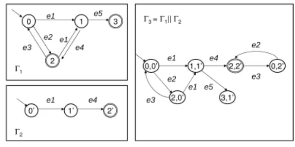
Example 1 In Figure 1,Γ1andΓ2are two automata. The
third oneΓ3is produced by synchronizingΓ1andΓ2.
0 1 2 e1 e1 e2 0’ 1’ 2’ Γ1 Γ2 Γ3 = Γ1|| Γ2 e1 e4 0,0’ 1,1’ e1 e4 2,2’ 0,2’ e3 e2 2,0’ e2 e1 e3 e5 3 e4 3,1’ e5 e3
Figure 1.An example of synchronization
Definition 5 A trajectory of an automaton is a path of con-tiguous states and transitions in the automaton that begins at an initial state and ends at a final state of the automaton.
Example 2 The trajectories in the automaton Γ3 in
Fig-ure 1 can be represented as the two formulas below, in which[ ]∗
means the content in[ ] repeated 0 or more times:
[(0, 0′)e2−→(2, 0′)→−e3]∗[(0, 0′)e1−→(1, 1′)→e4−(2, 2′)][e3−→(0, 2′)e2−→(2, 2′)]∗ , [(0, 0′ )e2−→(2, 0′)e3−→]∗[(0, 0′)→−e2(2, 0′)→e1−(1, 1′)→e4−(2, 2′)] [e3−→(0, 2′)e2−→(2, 2′)]∗. 2
Definition 6 Concatenationbetween two automataΓ1 =
hX1, Σ1, T1, I1, F1i and Γ2 = hX2, Σ2, T2, I2, F2i, with
Σ1∩ Σ2 = ∅ and F1∩ I2 6= ∅, produces an automaton
Γ = Γ1◦Γ2, whereΓ = hX1∪X2, Σ1∪Σ2, T1∪T2, I1, F2∪
(F1\I2)i.
3
Modeling Web Service Processes with
Discrete-Event Systems
3.1
Description of the Web Service
Pro-cesses
BPEL is an XML-based orchestration language devel-oped by IBM and recognized by OASIS [1]. BPEL is a so-called executable language because it defines the internal behaviour of a Web service process, as compared to chore-ography languages that define only the interactions among the Web services and are not executable. BPEL defines fif-teen activity types, among those the most important are the following:
P rocess ::= P rocess(Activity1, . . . , Activityn, V )
Activity ::= BasicActivity|StructuredActivity BasicActivity ::= receive|invoke|reply|assign|throw|
terminate|compensate|wait|empty StructuredActiviy ::= sequence|switch|f low|while|
pick|scope
Example 3 The loan approval process is an example de-scribed in the BPEL Specification 1.1 [1]. It is diagrammed in Figure 2. <receive> receive1 <invoke> invokeAssessor <invoke> invokeApprover <assign> assign <reply> reply receive_to_approval (request.amount>=1000) receive_to_assess (request.amount <1000) approval_to_reply assess_to_setMessage (risk.level=low) assess_to_approval (risk.level!=low) setMessage_to_reply input : request output : risk output: approval.accept=yes output: request input : request output : approval input: approval
Figure 2.A loan approval process. Activities are repsented in shaded boxes. The inV ar and outV ar are re-spectively the input and output variables of an activity.
This process contains five activities (big shaded blocks). An activity involves a set of input and output variables (dot-ted box besides each activity). All the variables are of composite type. The edges show the execution order of the activities. When two edges are issued from the same activity, only one edge that satisfies a triggering condition
(shown on the edge) will be activated. The process is trig-gered when ahreceivei activity named receive1 receives a message of a predefined type. First,receive1 initializes a variable request. Then, receive1 dispatches the request to one of the twohinvokei activities, invokeAssessor and invokeApprover, depending on the amount of the loan. In the case where the amount is large (request.amount >= 1000), invokeApprover is called for a decision, otherwise (request.amount < 1000), invokeAssessor is called for risk assessment. IfinvokeAssessor returns with an assess-ment that the risk level is low (risk.level = low), a reply is prepared by anhassigni activity and later sent out by a hreplyi activity, otherwise, invokeApprover is invoked for a final decision. The result frominvokeApprover is sent to the client by thehreplyi activity.
3.2
Modeling Web Services Process with
Discrete-Event Systems
A Web service process defined in BPEL is a composition of activities. We are going to model a BPEL activity as an automaton. A BPEL state is associated with an assignment of the variables. A BPEL activity is triggered when its ini-tial state satisfies a finite set of triggering conditions which is a certain assignment of variables. After an activity is ex-ecuted, the values of the state variables are changed. We need to extend the classic automaton definition to include the operations on state variables.
Assume a BPEL process has a finite set of variablesV = {v1, . . . , vn}, and the domain D = {D1, . . . , Dn} for V is
real values ℜ or arbitrary strings. C = {c1, . . . , cm} is a
finite set of constraints. A constraintcj of some arityk is
defined as a subset of the cartesian product over variables {vji, . . . , vjk} ⊆ V , i.e. cj ⊆ Dj1× · · · × Djk, or a first
order formula over{vji, . . . , vjk}. A constraint restricts the
possible values of thek variables.
A BPEL states is defined as an assignment of variables. A BPEL transition t is an operation on the state si, i.e.,
(sj, post(V2)) = t(si, e, pre(V1)), where V1 ⊆ V , V2 ⊆
V , pre(V1) ⊆ C is a set of preconditions that si has to
satisfy and post(V2) ⊆ C is a set of post-conditions that
the successor state sj will satisfy. If a states satisfies a
constraintc, we annotate as c ∧ s. Then, the semantics of transitiont is also represented as: t : (si∧ pre(V1))−→e(sj∧
post(V2)).
Definition 7 A BPEL activity is an automaton
hX, Σ, T, I, F, Ci, where C is the constraint set on variables
that define statesX and T : X × Σ × 2C→ X × 2C
.
3.2.1 Modeling Basic Activities
Due to lack of space, only major activities are included in this and the following subsection.
Activityhreceivei: h{so, sf}, {received}, {t}, {so}, {sf}, Ci
t : (so ∧ SoapM sg.type = M sgT ype)received−−−−−−→(sf ∧
RecM sg = SoapM sg), where
M sgT ype is a predefined message type. If the incoming message SoapM sg has the predefined type, RecM sg is initialized asSoapM sg.
Activityhreplyi : h{so, sf}, {replied}, {t}, {so}, {sf}, Ci
t : (so ∧ exists(RepM sg)) replied −−−−→(s
f ∧ SoapM sg =
RepM sg), where
exists(RepM sg) is the predicate checking that the replay messageRepM sg is initialized. SoapM sg is the message on the wire.
Activityhinvokei
Synchronous invocation (wait for a return message):
h{so, wait, sf}, {invoked, received}, {t1, t2}, {so}, {sf}, Ci
t1: (so∧ exists(InV ar))invoked−−−−−→(wait), and
t2: (wait)received−−−−−−→(sf ∧ exists(OutV ar)) where
InV ar and OutV ar are the input and output variables. Asynchronous invocation (not wait for a return message): h{so, sf}, {invoked}, {t}, {so}, {sf}, Ci
t : (so∧ exists(InV ar))invoked−−−−−→(sf).
Activityhassigni: h{so, sf}, {assigned}, {t}, {so}, {sf}, Ci
t : (so∧exists(InV ar)) assigned −−−−−−→(s
f∧OutV ar = InV ar)
Activityhthrowi: h{so, sf}, {thrown}, {t}, {so}, {sf}, Ci
t : (so∧ F ault.mode = Off )thrown−−−−−→(sf∧ F ault.mode =
On)
Activityhwaiti:
h{so, wait, sf}, {waiting, waited}, {t1, t2}, {so}, {sf}, Ci
t1 : (so ∧ W ait mode = Off) waiting
−−−−−→(wait ∧
W ait mode = On)
t2: (wait∧W ait mode = On)waited−−−−→(sf∧W ait mode =
Off)
This model is not temporal. We do not consider time, so the notion of delay is not considered in this activity.
Activityhemptyi: h{so, sf}, {empty}, {t}, {so}, {sf}, Ci
t : (so) empty −−−−→(s
f)
3.2.2 Modeling Structured Activities
Sequence Ahsequencei can nest n activities hAii in its scope. These activities are executed in sequential order. Assume hAii : hSAi, ΣAi, TAi, {sAio}, {sAif}, CAii, i ∈
{1, . . . , n}.
Activity hsequencei: h{so, sf} ∪ SSAi, {end} ∪
S {callAi} ∪ SΣAi, {ti} ∪ S TAi, {so}, {sf}, S CAii with t0: (so) callA1 −−−−→(sA 1o) ti: (sAif) callAi+1 −−−−−−→(sA i+1o) tn: (sAnf) end −−→(s f)
If assumeso= sA1o,sf = sAnf, andsAif = sAi+1o, for
i = [1, . . . , n − 1], a short representation of hsequencei is the concatenation of the nested activitiesA1◦ A2· · · ◦ An.
Switch Assume a hswitchi has n hcasei branches and one hotherwisei branch. Assume hAii :
hSAi, ΣAi, TAi, {sAio}, {sAif}, CAii, i ∈ {1, . . . , n + 1}.
Activity hswitchi: h{so, sf} ∪ SSAi, {end} ∪
S {switchAi} ∪ S ΣAi, S {tio} ∪ S {tif} ∪ S TAi, {so}, {sf}, S CAi∪ S pre(Vi)i.
Assume V1, . . . , Vn are variable sets on n hcasei
branches. The transitions are defined as below:
tio : (so ∧ ¬pre(V1) ∧ · · · ∧ pre(Vi) · · · ∧
¬pre(Vn)) switchAi
−−−−−−→(sA
io), ∀i ∈ {1, . . . n}
t(n+1)o(so ∧ ¬pre(V1) ∧ · · · ∧ ¬pre(Vi) · · · ∧
¬pre(Vn)) swicthAn+1 −−−−−−−−−→(s A(n+1)o) tif : (sAif) end −−→(s f), ∀i ∈ {1, . . . n + 1}
While Assume hwhilei nests an activity hAi: hSA, ΣA, TA, {sAo}, {sAf}, Ci.
Activity hwhilei: h{so, sf} ∪ SA, {while, while end} ∪
ΣA, {to, tf, t} ∪ TA, {so}, {sf}, C ∪ pre(W )i.
AssumeW is a variable set. to: (so∧ pre(W ))while−−−→(sAo)
tf : (so∧ ¬pre(W ))while end−−−−−−−→(sf)
t : (sAf)
ǫ − →(so)
Flow A hflowi can nest n activities hAii in its scope. These activities are executed concurrently. AssumehAii : hSAi, ΣAi, TAi, {sAio}, {sAif}, CAii, i ∈ {1, . . . , n}.
Activity hflowi: h{so, sf} ∪ SSAi, {start, end} ∪
S ΣAi, S {tio, tif} ∪STAi, {so}, {sf}, S CAii with tio: (so)start−−−→(sAio) tif : (sAif) end −−→(s f)
Notice that the semantic of automata cannot model con-currency. We actually model then-paralleled branches into n automata and define synchronization events to build their connections. The principle is illustrated in Figure 3. Each branch is modeled as an individual automaton. The entry statesoand the end statesf are duplicated in each branch.
Eventsstart and end are the synchronization events. More complicated case in joining the paralleled branches is dis-cussed in subsection 3.2.3. The key point in reasoning about decentralized automata is to postpone the synchronization until a synthesis result is needed, in order to avoid the state explosion problem. In Web service diagnosis, it is the situ-ation (cf. subsection 4.1).
Pick Assume a hpicki has n honMessagei and one honAlarmi branches. The correspondent branches are trig-gered by predefined events (for honMessagei) or by a time-out event produced by a timer (for honAlarmi). As-sume hAii : hSAi, ΣAi, TAi, {sAio}, {sAif}, CAii, i ∈ {1, . . . , n + 1}. Activity hpicki: h{so, sf} ∪ SSAi, S {startAi} ∪ {end} ∪SΣAi, S{t io, tif} ∪STAi, {so}, {sf}, SC Ai∪ S exists(eventAi)i with tio: (so∧ exists(eventAi)) startAi −−−−−→(s Aio) tif : (sAif) end −−→(s f) SA2o SA1o end SA1f SA2f event_A1 So So Sf start end event_A2 start Sf
Figure 3. Build concurrency as synchronized DES pieces.
3.2.3 Synchronization Links of Activities
Each BPEL activity can optionally nest the standard ele-mentshsourcei and htargeti:
< source linkN ame = “ncname”
transitionCondition = “bool − expr”?/ > < target linkN ame = “ncname”/ >
A pair ofhsourcei and htargeti defines a link which con-nects two activities. The target activity must wait until the source activity finishes. When onehflowi contains two par-allel activities which are connected by a link, the two activ-ities become sequentially ordered.
hsourcei can be modeled similarly like an hactivityi, with “transitionCondition” as the triggering condition.
Activityhsourcei: h{so, sf}, {ǫ}, {t}, {so}, {sf},
transitionConditioni with
t : (so∧ transitionCondition)−→ǫ(sf),
When an activity is thehtargeti of multiple links, a join condition is used to specify how these links can join. The join condition is defined within the activity. BPEL specifi-cation defines standard attributes for this activity:
<activityName=“ncname”, joinCondition=“bool-expr”, suppressJoinFailure=“yes—no”>
where joinCondition is the logical OR of the liveness status of all links that are targeted at this activity. If the condition is not satisfied, the activity is bypassed, and a fault is thrown if suppressJoinFailure is no.
In this case, the synchronization eventend as in Figure 3 is removed. If the ending state ofhflowi is the starting state s′
o of the next activity, the precondition of s ′
o is the
join-Condition. For example, either of the endings of the two
branches can trigger the next activity can be represented as: s′
o∧ (exists(sA1f) ∨ exists(sA2f)).
3.2.4 Modeling the Loan Approval Process
Example 4 The loan approval process in Example 3 contains five activities: hreceive1i, hinvokeAssessori, hinvokeApproveri, hassigni, hreplyi. The five ac-tivities are contained in a hflowi. Six links,
hreceive to assessi, hreceive to approvali, hassess to setMessagei, hassess to approvali, happroval to replyi,
and hsetMessage to replyi, connect the activities and
change the concurrent orders to sequential orders between the activities. In this special case, there are actually no concurrent activities. Therefore, for clarity, the event caused byhflowi is not shown. Assume the approver may
return an error message due to an unknown error. The formal representation of the process is shown on Figure 4(b)without highlights (the formulas are eliminated due to lack of space.)
4
Model-based Diagnosis for Web Service
Processes
A Web service process can run down for many reasons. For example, a composed Web service may be faulty, an in-coming message mismatches the interface, or the Internet is down. The symptom1of a failed Web service process is that exceptions are thrown and the process is halted. The current fault handling mechanism is throw-and-catch, sim-ilar to programming languages. The exceptions are thrown at the places where the process cannot be executed. The
catch clauses process the exceptions, normally to recover
the failure effects by executing predefined actions.
The throw-and-catch mechanism is very preliminary for fault diagnosis. The exception reports where it happened and returns some fault information. The exceptions can be regarded as associated with certain faults. When an ex-ception is thrown, we deduce that its associated fault oc-curred. This kind of association relations rely on the em-pirical knowledge of the developer. It may not be a real cause of the exceptions. In addition, there may exist mul-tiple causes of an exception which are unknown to the de-veloper. Therefore, the current throw-and-catch mechanism does not provide sound and complete diagnosis. For exam-ple, when a Web service throws an exception about a value in a customer order, not only the one that throws the excep-tion may be faulty, but the one that generates these data may
1In diagnosis concept, sympton is an observed abnormal behaviour,
while fault is the original cause of a sympton. For example, an alarm from a smoke detector is a symptom. The two possible faults, a fire or a faulty smoke detector, are the causes of the symptom.
also be faulty. But a Web service exception can only report the Web service where the exception happens with no way to know who generated these data. In addition, all the ser-vices that modified the data should be also suspected. Not all of this kind of reasoning is included in the current fault handling mechanism.
The diagnosis task is to determine the Web services re-sponsible for the exceptions. These Web services will be
diagnosed faulty. The exceptions come from the BPEL en-gine or the infrastructure below. We classify the exceptions into time-out exceptions and business logic exceptions.
The time-out exceptions are due to either a disrupted net-work or unavailable Web services. If there is a lack of re-sponse, we cannot distinguish whether the fault is in the network or at the remote Web service. Since we cannot diagnose which kind of faults prevent a Web service from responding, we can do little with time-out exceptions.
The business logic exceptions occur while invoking an external Web service and executing BPEL internal activi-ties. For example, mismatching messages (including the type of parameters and the number of parameters mismatch-ing) cause the exceptions to be thrown when the parameters are passed to the remote method. BPEL can throw excep-tions indicating the input data is wrong. During execution, the remote service may stop if it cannot process the request. The most common scenarios are the invalid format of the parameters, e.g. the data is not in a valid format, and the data is out of the range. The causes of the exceptions are various and cannot be enumerated. The common thread is that a business logic exception brings back information on the variables that cause the problem. In this paper, our ma-jor effort is on diagnosing business logic-related exceptions. So in our framework, COM P S is made up of all the basic activities of the Web service process considered, and OBS is made up of the exceptions thrown and the events of the executed activities. These events can be obtained by the monitoring function of a BPEL engine. A typical correct model for an activityhAi is thus:
¬ab(A) ∧ ¬ab(A.inputs) =⇒ ¬ab(A.outputs) (1) For facilitating diagnosis, the BPEL engine has to be ex-tended for the following tasks: 1) record the events emit-ted by execuemit-ted activities; 2) record the input and output SOAP messages; and 3) record the exceptions and trig-ger the diagnosis function when the first exception is re-ceived. Diagnosing is triggered on the first occurred ex-ception2. The MBD approach developed relies on the fol-lowing three steps with the techniques we introduced in the content above.
2When a Web service engine supports multiple instances of a process,
different instances are identified with a process ID. Therefore, diagnosis is based on the events for one instance of the process.
1) A prior process modelling and variable depen-dency analysis. All the variables in BPEL are global vari-ables, i.e. they are accessible by all the activities. An ac-tivity can be regarded as a function that takes input vari-ables and produces output varivari-ables. An activity has three kinds of relation to its input and output variables: initial-ization, modification and utilization. We useInit(A, V ), M od(A, V ) and U til(A, V ) to present the relation that ac-tivityA initializes V , modifies V or utilizes variable V . An activity is normally a utilizer of its input variables, and is ei-ther an initializer or an modifier of its output variables. This is similar to the view point of programming slicing, a tech-nique in software engineering for software debugging. But BPEL can violate this relation by applying some business logic. For example, some variables, such as order ID and customer address, are not changeable after they are initial-ized in a business process. Therefore, a BPEL activity may be an utilizer of its output variables. In BPEL, it is defined in correlation sets. In this case, we useU til(A, (V 1, V 2)) to express that outputV 2 is correlated to input V 1. In this case, Formula 1 can be simplified as:
¬ab(A.input) =⇒ ¬ab(A.output),
ifU til(A, (A.input, A.output)) (2) In Example 5, we give a table to summarize the variable dependency for the load approval process. This table can be obtained automatically from BPEL. The approach is not presented due to lack of space.
Example 5 The variable dependency analysis for the loan approval process is in Table 1.
2) Trajectories reconstruction from observations af-ter exceptions are detected. As mentioned earlier, the ob-servations are the events and exceptions when a BPEL pro-cess is executed. The events can be recovered from the log file in a BPEL engine. The observations are formed in an automaton. The trajectories are calculated by synchronizing the observations with the automaton of the system descrip-tion:
trajectories= SD||OBS (3) As trajectories can be recovered fromOBS, we do not require to record each event during the execution. It is very useful when some events are not observable and when there are too many events to record. It is our future work to study the minimal observables for diagnosing a fault.
Example 6 In the loan approval example, assume that OBS={received, invoked assessor, received risk, in-voked approver, received aplErr} (as in Figure 4(a)). received aplErr is an exception showing that there is a
Variables Parts Initializer Modifier Utilizer
request firstname receive1 invokeAssessor, invokeApprover
lastname receive1 invokeAssessor, invokeApprover
amount receive1 invokeAssessor, invokeApprover
risk level invokeAssessor
approval accept assign, invokeApprover reply error errorCode invokeApprover
Table 1.The variable dependency analysis for the loan approval process.
type mismatch in received parameters. We can build the trajectory of evolution as below, also shown in Figure 4(b).
(x0)received−−−−−−→(x1)→−ǫ(x2)invoked assessor−−−−−−−−−−−−−→(x4)received risk−−−−−−−−−→(x5) ǫ
−
→(x3)invoked approver−−−−−−−−−−−−−→(x7)received aplErr−−−−−−−−−−−−→(x8)
x0 invoked_assessor Invoked_approver received x2 received_risk x1 received_aplError x5 x3 x4 x0 x3 x6 x11 ε invoked_assessor x2 Invoked_approver assigned x9 x10 reply received x4 received_risk x8 x1 ε x5 ε ε x7 received_approval ε ε received_aplError (a) (b)
Figure 4.(a) the observations; (b) the loan approval pro-cess evolution trajectory up to the exception.
3) Accountability analysis for mode assignment
Not all the activities in a trajectory are responsible for the exception. As a software system, the activities connect to each other by exchanging variables. Only the activities which change the attributes within a variable can be respon-sible for the exception.
Assume that activityA generates exception ef, andt is a
trajectory ending atA. The responsibility propagation rules are (direct consequences of the contraposition of Formula 1 and 2):
∀A.InV ar.part ∈ A.InV ar,
ef ∈ ΣA ⊢ ab(A) ∨
_
ab(A.InV ar.part) (4) ∀Aj ∈ t, Aj 6= Ai, Aj is the only activity between
Aj and Ai such that M od(Aj, Ai.InV ar.part) ∨
Init(Aj, Ai.InV ar.part), ∀Aj.InV ar.part ∈
Aj.InV ar,
ab(Ai.InV ar.part) ⊢ ab(Aj)∨
_
ab(Aj.InV ar.part)
(5) The first rule in (4) states that if an activityA generates an exceptionef, it is possible that activityA itself is faulty,
or any part in itsA.InV ar is abnormal. Notice a variable is a SOAP message which has several parts.A.InV ar.part is a part inA.InV ar3. The second rule in (5) propagates
the responsibility backwards in the trajectory. It states that an activity Aj ∈ t that modifies or initializes a part of
Ai.InV ar which is known as faulty could be faulty; and
its inputs could also be faulty. If there are several activi-ties that modify or initialize a part ofAi.InV ar, only the
last one counts, because it overrides the changes made by the other activities, i.e.Ajis the last activity “between”Aj
and A that modifies or initializes Ai.InV ar, as stated in
(5). After responsibility propagation, we obtain a
responsi-ble set of activitiesRS = {Ai} ⊆ t.
Then the diagnosis is that either A or any of Ai in the
responsible set is faulty:
{Df} = {{A}} ∪ {{Ai}|Ai∈ RS} (6)
Each Df is a single fault diagnosis and the
re-sult is the disjunct of Df. The algorithm is as
fol-lowing. In the worst case, this algorithm checks each activity in t. In the worst case, the function getF irstM odAct(t, A, next part) checks each activity in t also. Assume k1 is the maximum number of variables
in an activity, andk2 is the maximum number of parts in
a variable. The worst case complexity of this algorithm isO(k1k2|t|2), but experiments on examples exhibit lower
real complexity.
3Sometimes, the exception returns the information about the part
A.InV ar.part is faulty. Then this rule is simplified.
Algorithm 1Calculate Diagnosis for a Faulty Web Service Process
INPUT: A0- the activity generating the exception.
t - a list of activities in a reserved trajectory whose first element is A0.
Acts - a list of candidate activities, initialized as{A0}.
OUTPUT: D - the list of faulty activities, initialized as{A0}.
Notes about the algorithm: 1) list.next() returns the first el-ement of a list; list.add(elel-ement) adds an elel-ement at the end of the list; list.remove(element) removes an element from the list. 2) Activity A has a list of variables A.V ars and a vari-able var = A.V ars.next() has a list of parts var.P arts. 3) getF irstM odAct(t, A, next part) is a function to return the first activity from A in t that modifies or initializes next part. whileActs! = null do
A= Acts.next()
fornext var In A.InV ars do fornext part In next var.parts do
B= getF irstM odAct(t, A, next part) ifB! = null then
D.add(B) Acts.add(B) Acts.remove(A) return D
Example 7 For the loan approval example, we have the trajectory as in Example 6. We do the responsibility propagation. As invokeApprover generates the
excep-tion, according to Formula (4), invokeApprover is
pos-sibly faulty. Then its input request is possibly faulty.
Among all the activities {receive1, invokeAssessor, invokeApprover} in the trajectory, receive1
initial-izesrequest, invokeAssessor and invokeApprover use request. Therefore, receive1 is possibly faulty, according
to Formula (5). receive1 is the first activity in the
trajec-tory. The propagation stops. The diagnosis is:
{Df} = {{receive1}, {invokeApprover}}
Example 7 has two single faults {receive1} and {invokeApprover} for the exception received aplErr, which means either the activity hreceive1i or hinvokeApproveri is faulty. In an empirical way, an engineer may associate only one fault for an exception. But our approach can find all possibilities. Second, if we want to further identify which activity is indeed responsible for the exception, we can do a further test on the data. For example, if the problem is wrong data format, we can verify the data format against some specification, and then identify which activity is faulty.
4.1
Multiple Exceptions
There are two scenarios where multiple exceptions can happen. The first scenario is the chained exceptions when one exception causes the others to happen. Normally the software reports this chained relation. We need to diagnose only the first occurred exception, because the causal rela-tions for other exceprela-tions are obvious from the chain.
The second scenario is the case when exceptions occur independently, e.g. two parallelled branches report excep-tions. As the exceptions are independent, we diagnose each exception independently, the synthesis diagnoses are the union of all the diagnoses. Assume the diagnoses for ex-ception 1 are {D1
i}, where i ∈ [1, . . . , n], and the
diag-noses for exception 2 are{D2
j}, where j ∈ [1, . . . , m], the
synthesis diagnoses are any combinations of D1
i andDj2:
{D1
i ∪ Dj2|i ∈ [1, . . . , n], j ∈ [1, . . . , m]}.
What interests us most is the synthesis of the minimal diagnoses. So, we remove theD1
i ∪ Dj2that are supersets
of other ones. This happens only if at least one activity is common to{D1
i} and {Dj2}, giving rise to a single fault that
can be responsible for both exceptions. Such activities are thus most likely to be faulty (single faults being preferred to double faults).
5
Related Work
MBD has been used for software debugging. Wotawa, among others, has used consistency-based diagnosis for de-bugging java and hardware description languages [7]. He has also discussed the relationship between MBD based de-bugging and program slicing [7] and concluded that MBD in his way and program slicing should draw equivalent con-clusions for debugging.
The diagnosis method developed in this paper can be compared to dynamic slicing introduced in [5]. Similar to our method, dynamic slicing considers the bugs should be within the statements that actually affect the value of a variable at a program point for a particular execution of the program. Their solution, following after Weiser’s static slicing algorithm [6], solves the problem using data-flow equations, which is also similar to the variable dependency analysis presented in this paper, but not the same. An exter-nal Web service can be seen as a procedure in a program, with unknown behaviour. For a procedure, we normally consider the outputs brought back by a procedure are gen-erated according to the inputs. Therefore, in slicing, the outputs are considered in the definition set (the set of the variables modified by the statement). For Web services, we can know some parts in SOAP response back from a Web service should be unchanged, e.g. the name and the address of a client. Therefore, the variable dependency analysis is
different from slicing. As a consequence, the diagnosis ob-tained from MBD approach in this paper can be different from slicing, and actually more precise.
Some other people have applied MBD on diagnosing component-based software systems. We found that when diagnosing such systems, the modelling is rather at the com-ponent level than translating lines of statements into logic representations. Grosclaude in [3] used a formalism based on Petri nets to model the behaviours of component-based systems. It is assumed that only some of the events are monitored. The history of execution is reconstructed from the monitored events by connecting pieces of activities into possible trajectories. Console’s group is working towards the same goal of monitoring and diagnosing Web services like us. In their paper [2], a monitoring and diagnosing method for choreographed Web service processes is devel-oped. Unlike BPEL in our paper, choreographed Web ser-vice processes have no central model and central monitor-ing mechanism. [2] adopted grey-box models for individual Web services, in which individual Web services expose the dependency relationships between their input and output pa-rameters to public. The dependency relationships are used by the diagnosers to determine the responsibility for excep-tions. This abstract view could be not sufficient when deal-ing with highly interactdeal-ing components. More specifically, if most of the Web services claim too coarsely that their outputs are dependent on their inputs, which is correct, the method in [2] could diagnose all the Web services as faulty. Yan et al. [8] was a preliminary work to the present one, fo-cusing on Web service modeling using transition systems. Our work simplifies the model and, more importantly, for-malizes the diagnosis principle and presents the diagnosis algorithm for Web service processes.
Other related research includes the studies on Web vice monitoring mechanism and the studies to map Web ser-vice processes into formal models. The discussion on these studies are eliminated due to lack of space.
6
Conclusions
To identify the Web services that are responsible for a failed business process is important for e-business applica-tions. Existing throw-and-catch fault handling mechanism is an empirical mechanism that does not provide sound and complete diagnosis. In this paper, we develop a monitor-ing and diagnosis mechanism based on solid theories in MBD. Automata are used to give a formal modelling of Web service processes described in BPEL. We adapt the existing MBD techniques for DES to diagnose Web ser-vice processes. Web serser-vice processes have all the features of software systems and do not function abnormally until an exception is thrown, which makes the diagnosis princi-ple different from diagnosing physical systems where fault
events are unobservable. The approach developed here re-constructs execution trajectories based on the model of the process and the observations from the execution. The vari-able dependency relations are utilized to deduce the actual Web services within a trajectory responsible for the thrown exceptions. The approach is sound and complete in the con-text of modelled behaviour. A BPEL engine can be ex-tended for the monitoring and diagnosis approach devel-oped in this paper.
References
[1] T. Andrews, F. Curbera, H. Dholakia, Y. Goland, and et.al. Business process execution lan-guage for Web Services (BPEL4WS) 1.1, 2003. ftp://www6.software.ibm.com/software/developer/library/ws-bpel.pdf, retrieved April 10, 2005.
[2] L. Ardissono, L. Console, A. Goy, G. Petrone, C. Pi-cardi, and M. Segnan. Cooperative model-based diag-nosis of web services. In Proceedings of the 16th
In-ternational Workshop on Principles of Diagnosis (DX-2005), pages 125–132, 2005.
[3] I. Grosclaude. Model-based monitoring of software components. In Proceedings of the 16th European
Conf. on Artificial Intelligence (ECAI’04), pages 1025–
1026, 2004.
[4] W. Hamscher, L. Console, and J. de Kleer, editors.
Readings in model-based diagnosis. Morgan Kauf-mann, 1992.
[5] B. Korel and J. Laski. Dynamic program slicing.
Infor-mation Processing Letters, 29(3):155–163, 1988.
[6] Mark Weise. Program slicing. IEEE Transactions on
Software Engineering, 10(4):352–357, 1984.
[7] Franz Wotawa. On the relationship between model-based debugging and program slicing. Artificial
Intelli-gence, 135:125–143, 2002.
[8] Y. Yan, Y. Pencol´e, M-O. Cordier, and A. Grastien. Monitoring web service networks in a model-based ap-proach. In 3rd IEEE European Conference on Web
Ser-vices (ECOWS05), V¨axj¨o, Sweden, Nov. 14-16, 2005.
IEEE Computer Society.