Modeling and Control of Manipulators - Part I: Geometric and Kinematic Models

HAL Id: cel-02129939

https://hal.inria.fr/cel-02129939

HAL is a multi-disciplinary open access archive for the deposit and dissemination of sci-entific research documents, whether they are pub-lished or not. The documents may come from teaching and research institutions in France or abroad, or from public or private research centers.

L’archive ouverte pluridisciplinaire HAL, est destinée au dépôt et à la diffusion de documents scientifiques de niveau recherche, publiés ou non, émanant des établissements d’enseignement et de recherche français ou étrangers, des laboratoires publics ou privés.

Distributed under a Creative Commons Attribution - NonCommercial| 4.0 International License

Geometric and Kinematic Models

Wisama Khalil

To cite this version:

Wisama Khalil. Modeling and Control of Manipulators - Part I: Geometric and Kinematic Mod-els. Doctoral. GdR Robotics Winter School: Robotica Principia, Centre de recherche Inria Sophia Antipolis – Méditérranée, France. 2019. �cel-02129939�

Modeling and Control of

Manipulators

Part I:

Geometric and Kinematic Models

Master I EMARO

European Master on Advanced Robotics

Wisama KHALIL

Ecole Centrale de Nantes

Master Automatique, Robotique et Informatique

Appliquée

Master in Control Engineering, Robotics and Applied

Informatics

2013-2014

Chapter 1: Terminology and general definitions

1.1. Introduction ...1

1.2. Mechanical components of a robot ...2

1.3. Definitions ... ………..4

1.3.1. Joints ... 4

1.3.2 Degrees of Mobility or Number of degrees of freedom of a body ...5

1.3.3. Joint space ... 5

1.3.4. Task space ... 5

1.3.5. Redundancy ...6

1.3.6. Singular configurations ...6

1.4. Choosing the number of degrees of freedom of a robot ... ………..7

1.5. Architectures of robot manipulators ... 7

1.6. Characteristics of a robot ...12

1.7. Conclusion ... …...13

Chapter 2: Transformation matrix between vectors, frames and screws Transformation matrix between vectors, frames and screws 2.1. Introduction ... 15

2.2. Homogeneous coordinates ... 16

2.2.1. Representation of a point ... ...16

2.2.2. Representation of a direction... ...16

2.2.3. Representation of a plane ... ... 17

2.3. Homogeneous transformations [Paul 81]... ... 17

2.3.1. Transformation of frames ... ... 17

2.3.2. Transformation of vectors ... ... 18

2.3.3. Transformation of planes ... ... 19

2.3.4. Transformation matrix of a pure translation ... ... 19

2.3.5. Transformation matrices of a rotation about the principle axes ... ...20

2.3.6. Properties of homogeneous transformation matrices ... ...22

2.3.7. Transformation matrix of a rotation about a general vector located at the origin . 25 2.3.8. Equivalent angle and axis of a general rotation ... 27

2.4. Representation of velocities ... ………..29

2.4.1. Definition of a screw ... ………30

2.4.2. Kinematic screw ... …………... 30

2.4.3. Transformation matrices between screws ... ……….31

2.5. Differential translation and rotation of frames ... ……… 32

2.6. Representation of forces (wrench) ... ………..35

Chapter 3: Direct geometric model of serial robots

3.1. Introduction ... 37

3.2. Description of the geometry of serial robots ... ………..38

3.3. Direct geometric model ... ………...44

3.4. Optimization of the computation of the direct geometric model ... ………..47

3.5. Transformation matrix of the end-effector in the world frame ... ………. 50

3.6. Specification of the orientation ... ………. 51

3.6.1. Euler angles ... …………... 52

3.6.2. Roll-Pitch-Yaw angles ... ……….54

3.6.3. Quaternions ... ……….56

3.7. Conclusion ... …………..…...58

Chapter 4: Inverse geometric model of serial robots 4.1. Introduction ... ………...59

4.2. Mathematical statement of the problem ... ………. 60

4.3. Inverse geometric model of robots with simple geometry ... ………..61

4.3.1. Principle ... ……… 61

4.3.2. Special case: robots with a spherical wrist ... ………63

4.3.3. Inverse geometric model of robots with more than six degrees of freedom ……..71

4.3.4. Inverse geometric model of robots with less than six degrees of freedom ……….71

4.4. Inverse geometric model of decoupled six degree-of-freedom robots ... 74

4.4.1. Introduction ... 74

4.4.2. Inverse geometric model of six degree-of-freedom robots with a spherical joint ..75

4.4.3. Inverse geometric model of robots with three prismatic joints ... ………82

4.5. Inverse geometric model of general 6 dof robots ... ………...83

4.6. Conclusion ... ………...87

Chapter 5: Direct kinematic model of serial robots 5.1. Introduction ... ……… 89

5.2. Computation of the Jacobian matrix from the direct geometric model ... ……….90

5.3. Kinematic Jacobian matrix ... ………..91

5.3.1. Computation of the kinematic Jacobian matrix ... ………92

5.3.2. Computation of the matrix iJn ... ………94

5.4. Decomposition of the Jacobian matrix into three matrices ... ………..97

5.5. Efficient computation of the end-effector velocity ... ………. 98

5.6. Dimension of the task space of a robot ... ………. 99

5.7. Analysis of the robot workspace ... ………..100

5.7.1. Workspace ... …………... 100

5.7.2. Singularity branches ... ………101

5.7.3. Jacobian surfaces ... ………104

5.7.4. Concept of aspect ... ………105

5.7.5. t-connected subspaces ... ………107

5.8. Velocity transmission between joint space and task space ... ………..110

5.8.1. Singular value decomposition ... ……… 110

5.9. Static model ... ………...114

5.9.1. Representation of a wrench ... ………... 114

5.9.2. Mapping of an external wrench into joint torques ... ………114

5.9.3. Velocity-force duality ... ……… 115

5.10. Second order kinematic model ... ………. 117

5.11. Kinematic model associated with the task coordinates representation .. ………..118

5.11.1. Direction cosines ... ………….. 119

5.11.2. Euler angles ... …………... 120

5.11.3. Roll-Pitch-Yaw angles ... ………121

5.11.4. Quaternions ... ………122

5.12. Conclusion ... ………. 122

Chapter 6: Inverse kinematic model of serial robots 6.1. Introduction ... ………...124

6.2. General form of the kinematic model ... ……….124

6.3. Inverse kinematic model for a regular case ... ……….125

6.3.1. First method ... ………126

6.3.2. Second method ... ………126

6.4. Solution in the neighborhood of singularities ... ………. 128

6.4.1. Use of the pseudoinverse ... ……… 129

6.4.2. Use of the damped pseudoinverse ... …………...130

6.4.3. Other approaches for controlling motion near singularities ... ………….. 132

6.5. Inverse kinematic model of redundant robots ... ………. 133

6.5.1. Extended Jacobian ... ………133

6.5.2. Use of the pseudoinverse of the Jacobian matrix ... ……… 135

6.5.3. Weighted pseudoinverse ... ……… 135

6.5.4. Pseudoinverse solution with an optimization term ... ………….. 136

6.5.5. Task-priority concept ... ……… 138

6.6. Numerical calculation of the inverse geometric problem ... ………. 141

6.7. Minimum description of tasks [Fournier 80], [Dombre 81] ... ………. 142

6.7.1. Principle of the description ... ……… 143

6.7.2. Differential models associated with the minimum description of Tasks ...146

6.8. Conclusion ... ……… 153

References... …………..467

Appendix 1: Solution of the inverse geometric model equations (Table 4.1)…..…………..497

Appendix 2: The inverse robot... …………503

Appendix 3: Dyalitic elimination ... …………505

Terminology and general definitions

1.1. Introduction

A robot is a mechanical device, containing electrically, electronically and IT parts. It possesses capacities of perception, action, decision, learning, communication and interaction with its environment, to realize certain tasks on the place of the man or in interaction with the man. Robotics is the field concerned with designing, constructing, integrating and programming robots.

Robots have been widely used with success in various industrial applications. Since the last two decades, other areas of application have emerged: medical, service (spatial, civil security, …), transport, underwater, entertainment, and even providing companionship in the form of artificial “pets” or humanoid robots. We can distinguish three main classes of robots: robot manipulators, which imitate the human arm, walking robots, which imitate the locomotion of humans, animals or insects, mobile robots, which look like cars, and flying robots “drones”.

The terms adaptability and versatility are often used to highlight the intrinsic flexibility of a robot. Adaptability means that the robot is capable of adjusting its motion to comply with environmental changes during the execution of tasks. Versatility means that the robot may carry out a variety of tasks – or the same task in different ways – without changing the mechanical structure or the control system.

A robot is composed of the following subsystems:

– mechanism: consists of an articulated mechanical structure actuated by electric, pneumatic or hydraulic actuators, which transmit their motion to the joints using suitable transmission systems;

– perception capabilities: They consist of the internal sensors that provide information about the state of the robot (joint positions and velocities), and the external sensors to obtain the information about the environment (contact

detection, distance measurement, artificial vision). They help the robot to adapt to disturbances and unpredictable changes in its environment;

– controller: realizes the desired task objectives. It generates the input signals for the actuators as a function of the user's instructions and the sensor outputs; – communication interface: through this the user programs the tasks that the

robot must carry out;

– workcell and peripheral devices: constitute the environment in which the robot works.

Robotics is thus a multidisciplinary science, which requires a background in mechanics, automatic control, electronics, signal processing, communications, computer engineering, etc.

The objective of this book is to present the techniques of the modeling, identification and control of robots. We restrict our study to rigid robot manipulators with a fixed base.

In this chapter, we will present certain definitions that are necessary to classify the mechanical structures and the characteristics of robot manipulators.

1.2. Mechanical components of a robot

The mechanism of a robot manipulator consists of two distinct subsystems, one (or more) end-effectors and an articulated mechanical structure:

– by the term end-effector, we mean any device intended to manipulate objects (magnetic, electric or pneumatic grippers) or to transform them (tools, welding torches, paint guns, etc.). It constitutes the interface with which the robot interacts with its environment. An end-effector may be multipurpose, i.e. equipped with several devices each having different functions;

– the role of the articulated mechanical structure is to place the end-effector at a given location (position and orientation) with a desired velocity and acceleration. The mechanical structure is composed of a kinematic chain of articulated rigid links. One end of the chain is fixed and is called the base. The end-effector is fixed to the free extremity of the chain. This chain may be serial (simple open chain) (Figure 1.1), tree structured (Figure 1.2) or closed (Figures 1.3 and 1.4). The last two structures are termed complex chains since they contain at least one link with more than two joints.

Figure 1.1. Simple open (or serial) chain

Serial robots with a simple open chain are the most commonly used. There are also industrial robots with closed kinematic chains, which have the advantage of being more rigid and accurate.

Figure 1.2. Tree structured chain

Figure 1.3. Closed chain

Figure 1.4 shows a specific architecture with closed chains, which is known as a parallel robot. In this case, the end-effector is connected to the base by several parallel chains [Inoue 85], [Fichter 86], [Reboulet 88], [Gosselin 88], [Clavel 89],

[Charentus 90], [Pierrot 91a], [Merlet 00]. The mass ratio of the payload to the robot is much higher compared to serial robots. This structure seems promising in manipulating heavy loads with high accelerations and realizing difficult assembly tasks.

Figure 1.4. Parallel robot

1.3. Definitions 1.3.1. Joints

A joint connects two successive links, thus limiting the number of degrees of freedom between them. The resulting number of degrees of freedom, m, is also called joint mobility, such that 0  m  6.

When m = 1, which is frequently the case in robotics, the joint is either revolute or prismatic. A complex joint with several degrees of freedom can be constructed by an equivalent combination of revolute and prismatic joints. For example, a spherical joint can be obtained by using three revolute joints whose axes intersect at a point.

1.3.1.1. Revolute joint

This limits the motion between two links to a rotation about a common axis. The relative location between the two links is given by the angle about this axis. The revolute joint, denoted by R, is represented by the symbols shown in Figure 1.5.

1.3.1.2. Prismatic joint

This limits the motion between two links to a translation along a common axis. The relative location between the two links is determined by the distance along this axis. The prismatic joint, denoted by P, is represented by the symbols shown in Figure 1.6.

Figure 1.6. Symbols of a prismatic joint

1.3.2 Mobility or Number of degrees of freedom of a body

The mobility of a body is defined as the number of independent components of its instantaneous velocity (rotational and linear), thus it is equal to 6 for a free body in space and 3 for a body in plane. In general it is  6.

1.3.3. Joint space E(q)

The space in which the location of all the links of a robot are represented is called joint space, or configuration space. We use the joint variables, q  N_{, as the}

coordinates of this space. Its dimension N is equal to the number of independent joints and corresponds to the number of degrees of freedom of the mechanical structure also known as the mobility of the structure. In an open chain robot (simple or tree structured), the joint variables are generally independent, whereas a closed chain structure implies constraint relations between the joint variables.

Unless otherwise stated, we will consider that a robot with N degrees of freedom has N actuated joints.

1.3.4. Task space E(X)

The location, position and orientation, of the end-effector is represented in the task space, or operational space. We may consider as many task spaces as there are end-effectors. Generally, Cartesian coordinates are used to specify the position in 3

3 _{x SO(3). An element of the task space is represented by the vector X  }M_{, where}

M is equal to the maximum number of independent parameters that are necessary to specify the location of the end-effector in space. Consequently, M  6 and M  N. In robot-manipulator (where holonomic joints are used) M is equal to the maximum mobility of the end-effector.

1.3.5. Redundancy

A robot is classified as redundant when the number of degrees of freedom of its joint space is greater than the number of degrees of freedom of its task space (N>M). Such robot can have an infinite number of configurations to locate the end effector at a desired location. This property increases the volume of the reachable workspace of the robot and enhances its performance. We will see in Chapter 6 that redundant robots can achieve a secondary optimum objective besides the primary objective of locating the end-effector.

Notice that a simple open chain is redundant if it contains any of the following combinations of joints (non-exhaustive):

– more than six joints;

– more than three revolute joints whose axes intersect at a point; – more than three revolute joints with parallel axes;

– more than three prismatic joints; – prismatic joints with parallel axes; – revolute joints with collinear axes. NOTES.–

– for an articulated mechanism with several end-effectors, redundancy is evaluated by comparing the number of degrees of freedom of the joint space acting on each end-effector and the number of degrees of freedom of the corresponding task space;

– a robot which is not redundant (N=M) may be redundant with respect to a particular task whose number of degrees of freedom, m, is less than the number of degrees of freedom of the robot.

– A robot is said to have redundant actuators if the number of motorized joints is greater than the number of degrees of freedom of the robot. This case may take place only in closed loop structures.

For all robots, redundant or not, it is possible that at some configurations, called singular configurations, the number of degrees of freedom of the end-effector becomes less than the dimension of the task space. For example, this may occur when:

– the axes of two prismatic joints become parallel; – the axes of two revolute joints become collinear;

In Chapter 5, we will present a mathematical condition to determine the number of degrees of freedom of the task space of a mechanism as well as its singular configurations.

1.4. Choosing the number of degrees of freedom of a robot

A non-redundant robot must have six degrees of freedom in order to place an arbitrary object in space. However, if the manipulated object exhibits revolution symmetry, five degrees of freedom are sufficient, since it is not necessary to specify the rotation about the revolution axis. In the same way, to locate a body in a plane, one needs only three degrees of freedom: two for positioning a point in the plane and the third to determine the orientation of the body.

From these observations, we deduce that:

– the number of degrees of freedom of a mechanism is chosen as a function of the shape of the object to be manipulated by the robot and of the class of tasks to be realized;

– a necessary but insufficient condition to have compatibility between the robot and the task is that the number of degrees of freedom of the end-effector of the robot is equal to or more than that of the task.

1.5. Architectures of robot manipulators

Without anticipating the results of the next chapters, we can say that the study of both tree structured and closed chains can be reduced to some equivalent simple open chains. Thus, the classification presented below is relevant for simple open chain architectures, but may also be generalized to the complex chains.

In order to count the possible architectures, we only consider revolute or prismatic joints whose consecutive axes are either parallel or perpendicular. Generally, with some exceptions (in particular, the last three joints of the GMF P150 and Kuka IR600 robots), the consecutive axes of currently used robots are either parallel or perpendicular. The different combinations of these four parameters yield the number of possible architectures with respect to the number of joints as shown in Table 1.1 [Delignières 87], [Chedmail 90a].

The first three joints of a robot are commonly designed in order to perform gross motion of the end-effector, and the remaining joints are used to accomplish orientation. Thus, the first three joints and the associated links constitute the shoulder or regional positioning structure. The other joints and links form the wrist.

Taking into account these considerations and the data of Table 1.1, one can count 36 possible combinations of the shoulder. Among these architectures, only 12 are mathematically distinct and non-redundant (we eliminate, a priori, the structures limiting the motion of the terminal point of the shoulder to linear or planar displacement, such as those having three prismatic joints with parallel axes, or three revolute joints with parallel axes). These structures are shown in Figure 1.7.

Table 1.1. Number of possible architectures as a function of the number of degrees of

freedom of the robot

Number of degrees of freedom of the robot

Number of architectures 2 8 3 36 4 168 5 776 6 3508

A survey of industrial robots has shown that only the following five structures [Liégeois 79] are manufactured:

– anthropomorphic shoulder represented by the first RRR structure shown in Figure 1.7, like PUMA from Unimation, Acma SR400, ABB IRBx400, Comau Smart-3, Fanuc (S-xxx, Arc Mate), Kuka (KR 6 to KR 200), Reis (RV family), Staübli (RX series), etc.;

– spherical shoulder RRP: "Stanford manipulator" and Unimation robots (Series 1000, 2000, 4000);

– RPR shoulder corresponding to the first RPR structure shown in Figure 1.7: Acma-H80, Reis (RH family), etc. The association of a wrist with one revolute degree of freedom of rotation to such a shoulder can be found frequently in the industry. The resulting structure of such a robot is called SCARA (Selective Compliance Assembly Robot Arm) (Figure 1.8). It has several applications, particularly in planar assembly. SCARA, designed by Sankyo, has been manufactured by many other companies: IBM, Bosch, Adept, etc.;

– cylindrical shoulder RPP: Acma-TH8, AFMA (ROV, ROH), etc.;

– Cartesian shoulder PPP: Acma-P80, IBM-7565, Sormel-Cadratic, Olivetti-SIGMA. More recent examples: AFMA (RP, ROP series), Comau P-Mast, Reis (RL family), SEPRO, etc.

The second RRR structure of Figure 1.7, which is equivalent to a spherical joint, is generally used as a wrist. Other types of wrists are shown in Figure 1.9 [Delignières 87].

A robot, composed of a shoulder with three degrees of freedom and a spherical wrist, constitutes a classical six degree-of-freedom structure (Figure 1.10). Note that the position of the center of the spherical joint depends only on the configuration of joints 1, 2 and 3. We will see in Chapter 4 that, due to this property, the inverse geometric model, providing the joint variables for a given location of the end-effector, can be obtained analytically for such robots.

According to the survey carried out by the French Association of Industrial Robotics (AFRI) and RobAut Journal [Fages 98], the classification of robots in France (17794 robots), with respect to the number of degrees of freedom, is as follows: 4.5% of the robots have three degrees of freedom, 27% have four, 9% have five and 59.5% have six or more. As far as the architecture of the shoulder is concerned, there is a clear dominance of the RRR anthropomorphic shoulder (65.5%), followed by the Cartesian shoulder (20.5%), then the cylindrical shoulder (7%) and finally the SCARA shoulder (7%).

RRR RRP

RPR

RPP PRR PPR PPP

Figure 1.7. Architectures of the shoulder (from [Milenkovic 83])

One-axis wrist

Two intersecting-axis wrist

Two non intersecting-axis wrist

Three intersecting-axis wrist (spherical wrist)

Three non intersecting-axis wrist

Figure 1.9. Architectures of the wrist (from [Delignières 87])

P

shoulder wrist

1.6. Characteristics of a robot

The standard ISO 9946 specifies the characteristics that manufacturers of robots must provide. Here, we describe some of these characteristics that may help the user in choosing an appropriate robot with respect to a given application:

– workspace: defines the space that can be reached by the end-effector. Its range depends on the number of degrees of freedom, the joint limits and the length of the links;

– payload: maximum load carried by the robot;

– maximum velocity and acceleration: determine the cycle time;

– position accuracy (Figure 1.11): indicates the difference between a commanded position and the mean of the attained positions when visiting the commanded position several times from different initial positions;

– position repeatability (Figure 1.11): specifies the precision with which the robot returns to a commanded position. It is given as the distance between the mean of the attained positions and the furthermost attained position;

– resolution: the smallest increment of movement that can be achieved by the joint or the end-effector.

However, other characteristics must also be taken into account: technical (energy, control, programming, etc.) and commercial (price, maintenance, etc.). Thus, the selection criteria are sometimes difficult to formulate and are often contradictory. To a certain extent, the simulation and modeling tools available in Computer Aided Design (CAD) packages may help in making the best choice [Dombre 88b], [Zeghloul 91], [Chedmail 92], [Chedmail 98].

Commanded position Position repeatability Position accuracy

1.7. Conclusion

In this chapter, we have presented the definitions of some technical terms related to the field of modeling, identification and control of robots. We will frequently come across these terms in this book and some of them will be reformulated in a more analytical or mathematical way. The figures mentioned here justify the choice of the robots that are taken as examples in the following chapters. In the next chapter, we present the transformation matrix concept, which constitutes an important mathematical tool for the modeling of robots.

Transformation matrix between vectors,

frames and screws

2.1. Introduction

In robotics, we assign one or more frames to each link of the robot and each object of the workcell. Thus, transformation of frames is a fundamental concept in the modeling and programming of a robot. It enables us to:

– compute the location, position and orientation of robot links relative to each other;

– describe the position and orientation of objects;

– specify the trajectory and velocity of the end-effector of a robot for a desired task;

– describe and control the forces when the robot interacts with its environment; – implement sensory-based control using information provided by various

sensors, each having its own reference frame.

In this chapter, we present a notation that allows us to describe the relationship between different frames and objects of a robotic cell. This notation, called homogeneous transformation, has been widely used in computer graphics [Roberts 65], [Newman 79] to compute the projections and perspective transformations of an object on a screen. Currently, this is also being used extensively in robotics [Pieper 68], [Paul 81]. We will show how the points, vectors and transformations between frames can be represented using this approach. Then, we will define the differential transformations between frames as well as the representation of velocities and forces using screws.

16

2.2. Homogeneous coordinates 2.2.1. Representation of a point

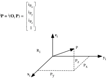
Let (i_P

x, iPy, iPz) be the Cartesian coordinates of an arbitrary point P with respect

to the frame R_i, which is described by the origin O_i and the axes x_i, y_i, z_i (Figure 2.1). The homogeneous coordinates of P with respect to frame R_i are defined by (wi_P

x, wiPy, wiPz, w), where w is a scaling factor. In robotics, w is taken to be equal

to 1. Thus, we represent the homogeneous coordinates of P by the (4x1) column vector: i_{P =} i_{(Oi P) =} x y z P P P i i i 1               [2.1] zi xi yi P Px Pz Py Ri

Figure 2.1. Representation of a point vector

2.2.2. Representation of a direction

A direction (free vector) is also represented by four components, but the fourth component is zero, indicating a vector at infinity. If the Cartesian coordinates of a unit vector u with respect to frame R_i are (i_ux, i_uy, i_{uz), its homogeneous coordinates}

will be: i_{u =} x y z u u u i i i 0               [2.2]

17

2.2.3. Representation of a plane

The homogeneous coordinates of a plane Q, whose equation with respect to a frame R_i is i_{x +} i_{y +} i_{z +} i_{ = 0, are given by:}

i_{Q =}

_[

_]

If a point P lies in the plane Q, then the matrix product i_Q i_{P is zero:}

i_Q i_{P =} x y z P P P i i i i i i i 1            _{  }         = 0 [2.4]

2.3. Homogeneous transformations [Paul 81] 2.3.1. Transformation of frames

The transformation, translation and/or rotation, of a frame R_i into frame R_j (Figure 2.2) is represented by the (4x4) homogeneous transformation matrix i_T

j such that: i_T j = isj inj iaj iPj = j j i i 0 0 0 1         R P [2.5a] where i_sj, i_{nj and} i_{aj contain the components of the unit vectors along the xj, yj and zj}

axes respectively expressed in frame Ri, and where iPj is the vector representing the

coordinates of the origin of frame R_j expressed in frame R_i.

We can also say that the matrix i_{Tj defines frame Rj relative to frame Ri.}

Thereafter, the transformation matrix [2.5a] will occasionally be written in the form of a partitioned matrix: i_{Tj =} i j i j 0 0 0 1         R P = i j i j i j i j 0 0 0 1         s n a P [2.5b]

18

Apparently, this is in violation of the homogeneous notation since the vectors have only three components. In any case, the distinction in the representation with either three or four components will always be clear in the text.

In summary: – the matrix i_T

j represents the transformation from frame Ri to frame Rj;

– the matrix i_{Tj can be interpreted as representing the frame Rj (three}

orthogonal axes and an origin) with respect to frame R_i.

iTj xi xj yj zj Ri Rj zi yi

Figure 2.2. Transformation of frames

2.3.2. Transformation of vectors

Let the vector j_{Pdefine the homogeneous coordinates of the point P with respect}

to frame R_j (Figure 2.3). Thus, the homogeneous coordinates of P with respect to frame R_i can be obtained as:

i_{P =} i_{(OiP) =} i_sj j_P x + inj jPy + iaj jPz + iPj = iTj jP [2.6] xi yj zj Ri Rj zi yi iTj P xj Oi

19 Thus the matrix i_T

j allows us to calculate the coordinates of a vector with respect

to frame R_i in terms of its coordinates in frame R_j.

•

j and jTi from Figure 2.4. Using equation

[2.5a], we directly obtain:

i_{Tj =} 0 0 1 3 0 1 0 12 1 0 0 6 0 0 0 1               , j_{Ti =} 0 0 1 6 0 1 0 12 1 0 0 3 0 0 0 1     _           6 3 12 zi xj xi zj yi yj Figure 2.4. Example 2.1 2.3.3. Transformation of planes

The relative position of a point with respect to a plane is invariant with respect to the transformation applied to the set of {point, plane}. Thus:

j_Q j_{P =} i_Q i_{P =} i_Q i_Tjj_P

leading to:

j_{Q =} i_Q i_{Tj [2.7]}

2.3.4. Transformation matrix of a pure translation

Let Trans(a, b, c) be this transformation, where a, b and c denote the translation along the x, y and z axes respectively. Since the orientation is invariant, the transformation Trans(a, b, c) is expressed as (Figure 2.5):

20 i_T j =Trans(a, b, c) = 1 0 0 a 0 1 0 b 0 0 1 c 0 0 0 1               [2.8]

From now on, we will also use the notation Trans(u, d) to denote a translation along an axis u by a value d. Thus, the matrix Trans(a, b, c) can be decomposed into the product of three matrices Trans(x, a) Trans(y, b) Trans(z, c), taking any order of the multiplication.

c a yj zi yi xj xi b zj

Figure 2.5. Transformation of pure translation

2.3.5. Transformation matrices of a rotation about the principle axes

2.3.5.1. Transformation matrix of a rotation about the x axis by an angle 

Let Rot(x, ) be this transformation. From Figure 2.6, we deduce that the components of the unit vectors i_s

j, inj, iaj along the axes xj, yj and zj respectively of

frame R_j expressed in frame R_i are as follows:







where S and C represent sin(and cos(respectively, and the superscript T indicates the transpose of the vector.

21 i_T j = Rot(x,) = 1 0 0 0 0 C S 0 0 S C 0 0 0 0 1    _                = 0 ( , ) 0 0 0 0 0 1               rot x [2.10]

where rot(x, ) denotes the (3x3) orientation matrix.

xi yi xj sj nj    yj zj zi aj

Figure 2.6. Transformation of a pure rotation about the x-axis 2.3.5.2. Transformation matrix of a rotation about the y axis by an angle 

In the same way, we obtain:

i_{Tj = Rot(y, ) =} C 0 S 0 0 1 0 0 S 0 C 0 0 0 0 1                   = 0 ( , ) 0 0 0 0 0 1               rot y  [2.11]

2.3.5.3. Transformation matrix of a rotation about the z axis by an angle  We can also verify that:

22 i_T j = Rot(z, ) = C S 0 0 S C 0 0 0 0 1 0 0 0 0 1                    = 0 ( , ) 0 0 0 0 0 1               rot z  [2.12]

2.3.6. Properties of homogeneous transformation matrices

a) From equations [2.5], a transformation matrix can be written as:

T = x x x x y y y y z z z z s n a P s n a P s n a P 0 0 0 1               = 0 0 0 1       R P [2.13]

The matrix R represents the rotation whereas the column matrix P represents the translation. For a transformation of pure translation, R = I₃ (I₃ represents the identity matrix of order 3), whereas P = 0 for a transformation of pure rotation. The matrix R represents the direction cosine matrix. It contains three independent parameters (one of the vectors s, n or a can be deduced from the vector product of the other two, for example s = n×a; moreover, the dot product n.a is zero and the magnitudes of n and a are equal to 1).

b) The matrix R is orthogonal, i.e. its inverse is equal to its transpose:

R-1 _{= R}T _[2.14]

c) The inverse of a matrix i_T

j defines the matrix jTi.

To express the components of a vector i_{P1 into frame Rj, we write:} j_P

1 = jTiiP1 [2.15]

If we postmultiply equation [2.6] by i_Tj-1 _{(inverse of} i_{Tj), we obtain:} i_T

j-1iP1 = jP1 [2.16]

From equations [2.15] and [2.16], we deduce that:

23 d) We can easily verify that:

Rot-1_{(u, ) = Rot(u, ) = Rot(–u, ) [2.18]}

Trans-1_{(u, d) = Trans(–u, d) = Trans(u, –d) [2.19]}

e) The inverse of a transformation matrix represented by equation [2.13] can be obtained as: T T T -1 T 0 0 0 1  _                   s P R n P T a P = T T 0 0 0 1  _        R R P _[2.20]

f) Composition of two matrices. The multiplication of two transformation matrices gives a transformation matrix:

T₁ T₂ = 1 1 2 2 0 0 0 1 0 0 0 1             R P R P = 1 2 1 2 1 0 0 0 1        R R R P P [2.21]

Note that the matrix multiplication is non-commutative (T₁T₂  T₂T₁).

g) If a frame R₀ is subjected to k consecutive transformations (Figure 2.7) and if each transformation i, (i = 1, …, k), is defined with respect to the current frame R_i-1, then the transformation 0_T

k can be deduced by multiplying all the transformation on

the right as:

0_{Tk =} 0_T11_T22_{T3 …} k-1_{Tk [2.22]}

h) If a frame R_j, defined by i_T

j, undergoes a transformation T that is defined

relative to frame R_i, then R_j will be transformed into R_j' with i_T

j' = T iTj (Figure

2.8).

From the properties g and h, we deduce that:

– multiplication on the right (postmultiplication) of the transformation i_Tj

indicates that the transformation is defined with respect to the current frame Rj;

– multiplication on the left (premultiplication) indicates that the transformation is defined with respect to the reference frame R_i.

24 1T2 z1 z0 k-1Tk x0 x1 y1 x2 y2 z2 xk-1 zk-1 yk zk 0T1 0Tk R0 R1 R2 Rk y0 yk-1 xk

Figure 2.7. Composition of transformations: multiplication on the right

xi yi zi _xj yj zj T iTj = iTj' Ri Rj zj' yj' xj' Ri' zi' yi' xi' Rj' T i'Tj' = iTj iTj

Figure 2.8. Composition of transformations: multiplication on the left

•

defined by:

0_{T2 = Rot(x,} 

6) Trans(y, d)

– reading 0_{T2 from left to right (Figure 2.9a): first, we apply the rotation; the}

new location of frame R0 is denoted by frame R1; then, the translation is

25 – reading 0_T

2 from right to left (Figure 2.9b): first we apply the translation, then

the rotation is defined with respect to frame R₀.

Trans(y, d) y0 z0 x2 y2 z2 y1 x0 x1 y1 z1 z0 a) b) x2 y2 z2 y0 x0, x1 z1 Rot(x, ₆) Rot(x, ₆) Trans(y, d) Figure 2.9. Example 2.2

i) Consecutive transformations about the same axis. We note the following properties:

Rot(u, ₁) Rot(u, ₂) = Rot(u, (₁ +₂)) [2.23]

Rot(u, ) Trans(u, d) = Trans(u, d) Rot(u, ) [2.24]

j) Decomposition of a transformation matrix. A transformation matrix can be decomposed into two transformation matrices, one represents a pure translation and the second a pure rotation:

T = ₌ 3 0 0 0 1 0 0 0 1 0 0 0 1                   R P I P R 0 [2.25]

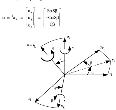
2.3.7. Transformation matrix of a rotation about a general vector located at the

origin

Let Rot(u,  be the transformation representing a rotation of an angle  about an axis, with unit vector u = [ux uy uz]T, located at the origin of frame Ri (Figure

2.10). We define the frame Rk such that zk is along the vector u and xk is along the

common normal between zk and zi. The matrix iTk can be obtained as: i_T

k = Rot(z, ) Rot(x, ) [2.26]

where  is the angle between x_i and x_k about z_i, and  is the angle between z_i and u about x_k.

26

From equation [2.26], we obtain:

u = x i k y z u S S a = u = C S C u       _{ }    _{ }   _{ }        [2.27]  xk xi yi yi' yk zi       u = zk

Figure 2.10. Transformation of pure rotation about any axis

The rotation about u is equivalent to the rotation about z_k. From properties g and h of § 2.3.6, we deduce that:

Rot(u, ) i_T

k = iTk Rot(z, ) [2.28]

thus:

Rot(u, ) = i_{Tk Rot(z, )} i_Tk-1

= Rot(z, ) Rot(x, ) Rot(z, ) Rot(x, –) Rot(z, –) [2.29] From this relation and using equation [2.27], we obtain:

Rot (u, ) = 0 ( , ) 0 0 0 0 0 1               rot u

27 = 2 x x y z x z y 2 x y z y y z x 2 x z y y z x z u (1-C )+C u u (1-C ) u S u u (1-C ) u S 0 u u (1-C ) u S u (1-C )+C u u (1-C ) u S 0 u u (1-C ) u S u u (1-C ) u S u (1-C )+C 0 0 0 0 1  _{ }     _{ }     _{ }                          [2.30]

We can easily remember this relation by writing it as:

rot(u,  = u uT (1 – C) + I3 C + ^u S [2.31]

where ^u indicates the skew-symmetric matrix defined by the components of the

vector u such that:

^_{u =} z y z x y x 0 u u u 0 u u u 0         _    [2.32]

Note that the vector product uxV is obtained by ^u V.

NOTES:-

- Rot(u, ) = i_T

k Rot(z, ) iTk-1, can be explained by the fact that iTk Rot(z, )

gives frame R_k with respect to frame R_i in its initial configuration. To find frame Ri after Rot(u, ), we have to multiply iTk Rot(z, ) by kTi.

2.3.8. Equivalent angle and axis of a general rotation 1

Let T be any arbitrary rotational transformation matrix such that:

1_{The Matlab function “U = vrrotmat2vec(R)” returns a 4x1 vector representing}

an axis-angle representation of rotation defined by the 3x3 matrix R. The first three components of U give the coordinates of the rotation axis and the fourth component gives the angle.

28 x x x y y y z z z s n a 0 s n a 0 s n a 0 0 0 0 1                T [2.33]

We solve the following expression for u and:

Rot (u,) = T with 0   

Adding the diagonal terms of equations [2.30] and [2.33], we obtain:

C = 1_{2 (sx} + n_y + a_z – 1) [2.34]

From the off-diagonal terms, we obtain:

x z y y x z z y x 2u S n a 2u S a s 2u S s n       _   _     [2.35] yielding: 2 2 2 z y x z y x 1 S (n a ) (a s ) (s n ) 2       [2.36]

From equations [2.34] and [2.36], we deduce that:

 = atan2 (S,C) with 0     [2.37] u_x, u_y and u_z are calculated using equation [2.35] if S  When S is small,

the elements u_x, u_y and u_z cannot be determined with good accuracy by this equation. However, in the case where C < 0, we obtain u_x, u_y and u_z more accurately using the diagonal terms of Rot(u,) as follows:

y x z x y z n C s C a C u , u , u 1 C 1 C 1 C         _          [2.38]

29 x x z y y y x z z z y x s C u sign(n a ) 1 C n C u sign(a s ) 1 C a C u sign(s n ) 1 C          _   _  _             [2.39]

where sign(.) indicates the sign function of the expression between brackets, thus sign(e) = +1 if e  0, and sign(e) = 1 if e < 0.

•

E

to the location Rot(y, /4) Rot(z, /2). We can write:

Rot(x, – /4) Rot(u, ) = Rot(y, /4) Rot(z, /2)

Thus:

Rot(u, ) = Rot(x, /4) Rot(y, /4) Rot(z, /2)

= 0 1/ 2 1/ 2 0 1/ 2 1/ 2 1/ 2 0 1/ 2 1/ 2 1/ 2 0 0 0 0 1                 

Using equations [2.34] and [2.36], we get: C = 1 2  , S = 3 2 , giving  = 2/3. Equation [2.35] yields: u_x = 1 3, uy = 0, uz = 2 3 . 2.4. Representation of velocities

In this section, we will use the concept of screw to describe the velocity of a body in space.

30

2.4.1. Definition of a screw

A vector field, H, on 3 _{is a screw if there exist a point O}

i and a vector  such

that for all points O_j in 3_:

Hj = Hi + x OiOj

where H_j is the vector of H at O_j and the symbol x indicates the vector product;  is called the vector of the screw of H. The vector H_j is also called the moment at O_j, whereas is also called the resultant of the screw.

Then, it is easy to prove that for every couple of points O_k and O_m:

H_m = H_k + x O_kO_m

Thus, the screw at a point O_i is well defined by the vectors H_i and , which can be concatenated in a single (6x1) vector.

2.4.2. Kinematic screw

Since the set of velocity vectors at all the points of a body defines a screw field, the screw at a point O_i can be defined by:

• v_i representing the linear velocity at O_{i with respect to the fixed frame R0}, such that vi = _dt(Od 0Oi);

• _{i representing the angular velocity of the body with respect to frame R0}. It constitutes the vector of the screw of the velocity vector field.

Thus, the velocity of a point O_j is calculated in terms of the velocity of the point O_i by the following equation:

j = +i i i j

v v ω O O [2.40]

The components of v_i and _i can be concatenated to form the kinematic screw vector V_i, i.e.:

T

T T

i = _ i i _

31 The kinematic screw is also called twist.

2.4.3. Transformation matrices between screws

Let i_v

i and ii be the vectors representing the kinematic screw in Oi, origin of

frame R_i, expressed in frame R_i. To calculate j_v

j and jj representing the kinematic

screw in O_j expressed in frame R_j, we first note that:

_j = i [2.42]

v_j = v_i + _i x L_i,j [2.43]

L_i,j being the position vector connecting O_i to O_j. Equations [2.42] and [2.43] can be rewritten as:

j , i j ˆ             _{ }           3 i j i 3 3 v _{I L v} 0 I   [2.44]

where I3 and 03 represent the (3x3) identity matrix and zero matrix respectively.

Projecting this relation in frame Ri, we obtain:

j j i i i i i ˆ i    _          _ _{ } _   V _{3 j} 3 3 i V I P 0 I   [2.45]

Since j_{vj =} j_Rii_{vj and} j_{j =} j_Rii_{j, equation [2.45] gives:}

j_V

j = jSi iVi [2.46]

where j_T

i is the (6x6) transformation matrix between screws:

j i j i i j j i j 3 i ˆ =          R R P S 0 R [2.47]

The transformation matrices between screws have the following properties: i) product:

32 0_{Sj =} 0_S1 1 _{S2 . . .} j-1_{S j [2.48]} ii) inverse: i i i j j j i j i 3 j ˆ           R P R S S 0 R - 1 j i _[2.49]

Note that equation [2.49] gives another possibility, other than equation [2.45], to define the transformation matrix between screws.

From [2.49] and [2.49], we can write:

i i j i i i j j j j j i i j _{i i} 3 j 3 j ˆ  _ ˆ                  R P R R R P S 0 R 0 R

2.5. Differential translation and rotation of frames

The differential transformation of the position and orientation – or location – of a frame Ri attached to any body may be expressed by a differential translation vector

dPi expressing the translation of the origin of frame Ri, and of a differential rotation

vector i, equal to ui d, representing the rotation of an angle d about an axis, with

unit vector ui, passing through the origin Oi.

Given a transformation i_{Tj, the transformation} i_{Tj + d}i_{Tj can be calculated,}

taking into account the property h of § 2.3.6, by the premultiplication rule as:

i_T

j + diTj = Trans(idxi, idyi, idzi) Rot(iui, d) iTj [2.50]

Thus, the differential of i_{Tj is equal to:}

di_T

j = [Trans(idxi, idyi, idzi) Rot(iui, d) – I4] iTj [2.51]

In the same way, the transformation i_{Tj + d}i_{Tj can be calculated, using the}

postmultiplication rule as:

i_{Tj + d}i_{Tj =} i_{Tj Trans(}j_dxj, j_dyj, j_{dzj) Rot(}j_{uj, d) [2.52]}

and the differential of i_T

33

di_{Tj =} i_{Tj [Trans(}j_dxj, j_dyj, j_{dzj) Rot(}j_{uj, d) – I4] [2.53]}

From equations [2.51] and [2.53], the differential transformation matrix  is defined as [Paul 81]:

 = [Trans(dx, dy, dz) Rot(u, d) – I₄] [2.54]

such that:

di_{Tj =} i_ i_{Tj [2.55]}

or:

di_T

j = iTjj [2.56]

Assuming that d is sufficiently small so that S(d) ≈ d and C(d) ≈ 1, the transformation matrix of a pure rotation d about an axis of unit vector u can be calculated from equations [2.30] and [2.54] as:

j_{ =} jˆj j j 0 0 0 0         dP  ₌













where u^ and ^ represent the skew-symmetric matrices defined by the vectors u and respectively.

Note that the transformation matrix between screws can also be used to transform the differential translation and rotation vectors between frames:

























_i the differential screw.

•

displacement. The differential model calculates the joint increments corresponding to the desired elementary displacement of frame R_n fixed to the terminal link (Figure 2.11). However, the task of the robot is often described in the tool frame R_E,

34

which is also fixed to the terminal link. The problem is to calculate n_dP

n and nn in

terms of E_dP

E and EE.

Let the transformation describing the tool frame in frame R_n be:

n_{TE =} 0 1 0 0 1 0 0 0.1 0 0 1 0.3 0 0 0 1   _            

and that the value of the desired elementary displacement is:

E_{dPE =}









n_{n =} n_REE_{E ,} n_{dPn =} n_{RE (}E_ExE_{Pn +} E_dPE)

The numerical application gives:

n_{dPn =}





0 0.015 0.005 , n_n =

[

]

In a similar way, we can evaluate the error in the location of the tool frame due to errors in the position and orientation of the terminal frame. Suppose that the position error is equal to 10 mm in all directions and that the rotation error is estimated as 0.01 radian about the x axis:

35

n_{dPn =}

_[

_]





0.01 0 0 The error on the tool frame is calculated by:

E_

E = ERnnn, EdPE = ERn (nnxnPE + ndPn)

which results in:

E_{dPE =}





0.013 0.01 0.011

 , E_{E =}





0 0.01 0

2.6. Representation of forces (wrench)

A collection of forces and moments acting on a body can be reduced to a wrench

F_i at point O_i, which is composed of a force f_i at O_i and a moment m_i about O_i:

Fi = i i       f m [2.59]

Note that the vector field of the moments constitutes a screw where the vector of the screw is fi. Thus, the wrench forms a screw.

Consider a given wrench i_{Fi, expressed in frame Ri. For calculating the}

equivalent wrench j_{Fj, we use the transformation matrix between screws such that:} j j j j         m f = j_S i i i i i         m f [2.60] which gives: j_{fj =} j_Ri i_{fi [2.61]} j_{mj =} j_{Ri (}i_fixi_{Pj +} i_{mi) [2.62]}

It is often more practical to permute the order of fi and mi. In this case, equation

[2.60] becomes:

























36

•

E describing the location of the tool

frame with respect to the terminal frame be:

n_{TE =} 0 1 0 0 1 0 0 0.1 0 0 1 0.5 0 0 0 1   _           

Supposing that we want to exert a wrench E_F

E with this tool such that EfE =

[0 0 5]T _and E_m

E = [0 0 3]T, determine the corresponding wrench nFn at the

origin O_n and referred to frame R_n. Using equations [2.61] and [2.62], it follows that:

n_f

n = nREEfE

n_{mn =} n_{RE (}E_fExE_Pn+ E_mE)

The numerical application leads to:

n_f

n =





n =





2.7. Conclusion

In the first part of this chapter, we have developed the homogeneous transformation matrix. This notation constitutes the basic tool for the modeling of robots and their environment. Other techniques have been used in robotics: quaternion [Yang 66], [Castelain 86], (3x3) rotation matrices [Coiffet 81] and the Rodrigues formulation [Wang 83]. Readers interested in these techniques can consult the given references.

We have also recalled some definitions about screws, and transformation matrices between screws, as well as differential transformations. These concepts will be used extensively in this book. In the following chapter, we deal with the problem of robot modeling.

Direct geometric model of serial robots

3.1. Introduction

The design and control of a robot requires the computation of some mathematical models such as:

– transformation models between the joint space (in which the configuration of the robot is defined) and the task space (in which the location of the end-effector is specified). These transformation models are very important since robots are controlled in the joint space, whereas tasks are defined in the task space. Two classes of models are considered:

– direct and inverse geometric models, which give the location of the end-effector as a function of the joint variables of the mechanism and vice versa;

– direct and inverse kinematic models, which give the velocity of the end-effector as a function of the joint velocities and vice versa;

– dynamic models giving the relations between the input torques or forces of the actuators and the positions, velocities and accelerations of the joints. The automatic symbolic computation of these models has largely been addressed in the literature [Dillon 73], [Khalil 76], [Zabala 78], [Kreuzer 79], [Aldon 82], [Cesareo 84], [Megahed 84], [Murray 84], [Kircánski 85], [Burdick 86], [Izaguirre 86], [Khalil 89a]. The algorithms presented in this book have been used in the development of the software package SYMORO+ [Khalil 97], which deals with all the above-mentioned models.

The modeling of robots in a systematic and automatic way requires an adequate method for the description of their structure. Several methods and notations have been proposed [Denavit 55], [Sheth 71], [Renaud 75], [Khalil 76], [Borrel 79], [Craig 86a]. The most popular among these is the Denavit-Hartenberg method

[Denavit 55]. This method is developed for serial structures and presents ambiguities when applied to robots with closed or tree chains. For this reason, we will use the notation of Khalil and Kleinfinger [Khalil 86a], which gives a unified description for all mechanical articulated systems, including mobile robots [Venture 2006], with a minimum number of parameters. In this chapter, we will present the geometric description and the direct geometric model of serial robots. Tree and closed loop structures will be covered in Chapter 7.

3.2. Description of the geometry of serial robots

A serial robot is composed of a sequence of n + 1 links and n joints. The links are assumed to be perfectly rigid. The links are numbered such that link 0 constitutes the base of the robot and link n is the terminal link (Figure 3.1). Joint j connects link j to link j – 1 and its variable is denoted q_j. The joints are either revolute or prismatic and are assumed to be ideal (no backlash, no elasticity). A complex joint can be represented by an equivalent combination of revolute and prismatic joints with zero-length massless links. In order to define the relationship between the location of links, we assign a frame R_j attached to each link j, such that:

– the zj axis is along the axis of joint j;

– the x_j axis is aligned with the common normal between z_j and z_j+1:

. if zj and zj+1 are collinear xj is not unique, it can be taken in any plane

perpendicular to them,

. if z_j and z_j+1 are parallel, x_j is not unique, it is in the plane defined by them,

. in the case of intersecting joint axes, xj is normal to the plane defined by

them and passing through their intersection point;

– the intersection of x_j and z_j defines the origin O_j, the y_j axis is formed by the right-hand rule to complete the coordinate system (x_j, y_j, z_j).

Link 1 Link 0 Link 2 Link 3 Link_n

Figure 3.1. Robot with simple open structure

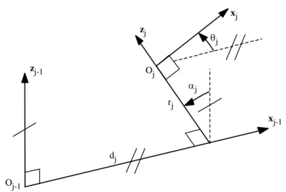
The transformation matrix from frame Rj-1 to frame Rj is expressed as a function

of the following four geometric parameters (Figure 3.2): • _j: the angle between z_j-1 and z_j about x_j-1; • dj: the distance between zj-1 and zj along xj-1;

• _j: the angle between x_j-1 and x_j about z_j; • rj: the distance between xj-1 and xj along zj.

z_j-1 x_j-1 z_j x_j d_j r_j _j _j O_j O_j-1

Figure 3.2. The geometric parameters in the case of a simple open structure The variable of joint j, defining the relative orientation or position between links j – 1 and j, is either _j or r_j, depending on whether the joint is revolute or prismatic respectively. This is defined by the relation:

j j j j j q =   +  r [3.1a] with: • _j = 0 if joint j is revolute; • _j = 1 if joint j is prismatic; • _j= 1 – _j.