radiation
M. Mihoviloviˇc,1, 2 A. B. Weber,1 P. Achenbach,1 T. Beranek,1 J. Beriˇciˇc,2 J. C. Bernauer,3R. B¨ohm,1 D. Bosnar,4 M. Cardinali,1 L. Correa,5L. Debenjak,2 A. Denig,1 M. O. Distler,1 A. Esser,1 M. I. Ferretti Bondy,1H. Fonvieille,5
J. M. Friedrich,6 I. Friˇsˇci´c,4 K. Griffioen,7 M. Hoek,1 S. Kegel,1 Y. Kohl,1 H. Merkel,1, ∗ D. G. Middleton,1 U. M¨uller,1 L. Nungesser,1 J. Pochodzalla,1 M. Rohrbeck,1 S. S´anchez Majos,1 B. S. Schlimme,1 M. Schoth,1 F. Schulz,1 C. Sfienti,1 S. ˇSirca,8, 2 S. ˇStajner,2 M. Thiel,1 A. Tyukin,1 M. Vanderhaeghen,1 and M. Weinriefer1
(A1-Collaboration) 1
Institut f¨ur Kernphysik, Johannes Gutenberg-Universit¨at Mainz, DE-55128 Mainz, Germany
2Joˇzef Stefan Institute, SI-1000 Ljubljana, Slovenia 3
Massachusetts Institute of Technology, Cambridge, MA 02139, USA
4
Department of Physics, University of Zagreb, HR-10002 Zagreb, Croatia
5Universit´e Clermont Auvergne, CNRS/IN2P3, LPC, BP 10448, F-63000 Clermont-Ferrand, France 6
Technische Universit¨at M¨unchen, Physik Department, 85748 Garching, Germany
7
College of William and Mary, Williamsburg, VA 23187, USA
8Faculty of Mathematics and Physics, University of Ljubljana, SI-1000 Ljubljana, Slovenia
(Dated: August 7, 2018)
We report on a new experimental method based on initial-state radiation (ISR) in e-p scattering, in which the radiative tail of the elastic e-p peak contains information on the proton charge form factor (GpE) at extremely small Q2. The ISR technique was validated in a dedicated experiment using the spectrometers of the A1-Collaboration at the Mainz Microtron (MAMI). This provided first measurements of GpE for 0.001 ≤ Q2≤ 0.004 (GeV/c)2
.
PACS numbers: 12.20.-m, 25.30.Bf, 41.60.-m
INTRODUCTION
The radius of the proton as a fundamental subatomic constant has recently received immense attention. The CODATA [1] value of 0.8751(61) fm was compiled from electron scattering and atomic Lamb shift measurements. Both approaches gave consistent results. This value how-ever, does not agree with the findings of very precise Lamb shift measurements in muonic hydrogen [2, 3], which are 6 σ away from the CODATA value. This dis-crepancy cannot be explained within existing physics the-ories, nor can it be interpreted as an experimental error. To provide further insight into the matter, several new spectroscopic and scattering experiments are underway. They aim to investigate different aspects of the prob-lem [4, 5].
In a scattering experiment the charge radius of the pro-ton is typically determined by measuring cross sections for elastic scattering of electrons from hydrogen, which depend on GpE and carry information about the charge distribution in the proton. The proton charge radius is given by r2p≡ −6¯h2 dGpE dQ2 Q2=0 , (1)
where Q2 is the negative square of the four-momentum transferred to the hadron. Due to the limited reach of existing data sets (Q2> 0.004 GeV2/c2) the slope of Gp
E at Q2= 0 needs to be evaluated from an extrapolated fit
of the measured data. The available data have enough resolving power to precisely determine the slope of the form factor at some distance from the origin, but addi-tional data are needed to constrain the slope at Q2= 0. Therefore, measurements of GpE need to be extended into the previously unmeasured region of Q2<
∼ 10−3GeV2/c2. Efforts to do such measurements with the standard ap-proaches are limited by the minimal Q2 accessible with the experimental apparatus at hand. The energy of the electron beam and the scattering angle must be very small. Here we present a new experimental approach that avoids these kinematic limitations, extends the currently accessible Q2 range, and allows for cross section mea-surements below 0.004 GeV2/c2 with sub-percent preci-sion. The initial state radiation (ISR) technique exploits information within the radiative tail of the elastic peak. This was inspired by a similar concept used in particle physics to measure e+e− → hadrons over a wide range of center-of-mass energies in a single experiment [6, 7].
INITIAL STATE RADIATION TECHNIQUE
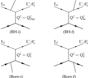
The radiative tail of an elastic peak is dominated by the contributions from two Bethe-Heitler diagrams [8] as shown in Fig. 1. The initial-state radiation (BH-i) cor-responds to the incident electron emitting a real photon before interacting with the proton, and the final-state ra-diation (BH-f) corresponds to a real photon being emit-ted after the interaction with the nucleon. For these
Q2= Q2 Out Q2= Q2In (BH-i) (BH-f) Q2= Q2 0 Q2= Q20 (Born-i) (Born-f) E0 E0, θe0 E0 E0, θe0 E0 E0, θe0 E0 E0, θe0
FIG. 1. Feynman diagrams for inelastic scattering of an elec-tron from a proton, where an elecelec-tron or a proton emits a real photon before or after the interaction. Diagrams where electrons emit a photon are known as Bethe-Heitler (BH) diagrams, while those where protons emit real photons are called Born diagrams. Q2In is the squared four-momentum
fixed by the beam energy and the scattering angle, while Q2Out≤ Q
2
In corresponds to the value measured with the
de-tector. Q20= 4E0E0sin2(θ0e/2)/c2, where E0 is the energy of
the incident electron, E0 and θe0 are the energy and angle of
the detected electron. For the (BH-i) diagram Q2 = Q2Out,
and for the (BH-f) diagram Q2= Q2In.
cesses two characteristic Q2can be defined: Q2 In= 4E02 c2 sin 2 θ0e 2 1 + 2E0 M c2sin 2 θ0 e 2 and Q2 Out = 4Ec202sin 2 θ0e 2 1− 2E0 M c2sin 2 θ0 e 2 . Here, Q2
Inrepresents the value set by the chosen kinemat-ics for elastic scattering (E0, θ0e), while Q2Out corresponds to the value measured by the detectors after scattering. E0and E0 are the energies of the incoming and scattered electrons, M is the mass of the proton, and θ0
eis the scat-tering angle of the detected electron. In the limit of exact elastic H(e, e0)p scattering, Q2
In and Q2Out are both equal to Q2
0 = 4E0E0sin2(θ0e/2)/c2 and correspond to the Q2 actually transferred to the proton. In H(e, e0)γp, how-ever, Q2
Inand Q2Outno longer coincide. In the initial-state radiation diagram the emitted photon carries away part of the incident electron’s four-momentum and opens the possibility to probe the proton’s electromagnetic struc-ture at Q2 = Q2
Out which is smaller than Q2In. On the other hand, in the final-state radiation diagram the mo-mentum transfer at the vertex remains fixed (Q2= Q2
In), thus only Q2Out is modified, Q2Out≤ Q2.
In an inclusive (e, e0) experiment only Q2
Out can be measured, which implies that initial state radiation can-not be distinguished from final state radiation. The mea-sured radiative tail represents an approximately 2 : 3 mixture of terms with Q2= Q2
Inand Q2= Q2Out, respec-tively. There are also Born terms (Born-i and Born-f),
where the initial and final protons emit real photons, as well as higher-order radiative corrections that also con-tribute to the radiative tail. The basic concept of the ISR approach is to isolate the interesting (BH-i) process from other contributions to the radiative tail, and thus ob-tain information on form factors at unmeasured values of Q2= Q2
Out. To accomplish this, the measurements need to be studied in conjunction with a Monte-Carlo simu-lation that encompasses a comprehensive description of the radiative tail.
DESCRIPTION OF THE RADIATIVE TAIL
To realistically mimic the radiative tail, the peaking approximation models devised from the corrections to the elastic cross section are insufficient [8]. For an adequate description far away from the elastic line (Q2= Q2
Out
Q2
In), it is crucial to consider cross-section contributions to the e8-order. To achieve this goal, a Monte-Carlo sim-ulation is used, which employs a sophisticated event gen-erator that calculates amplitudes exactly for the leading, e3-order diagrams (shown in Fig. 1) and includes Gp
E as a free, tuneable parameter for every simulated Q2. The next order vacuum polarization diagrams (with electrons inside the fermion loop) are exactly calculable and are added as a multiplicative factor to the cross section. The virtual corrections to the Bethe-Heitler diagrams (self-energy corrections and various vertex corrections) require integration of the loop diagrams and are computationally too intensive to be added directly to the simulation. In-stead they are considered as effective corrections to the cross section using the prescription of Ref. [8], together with the real second-order correction (emission of two real photons) which is approximated using the correc-tions to the elastic cross section [8, 9]. Hadronic cor-rections are also considered in the elastic limit using the calculations of Ref. [9]. They contribute only up to 0.5 % to the cross section at the lowest energy settings. In the simulation the proton is always on-shell. Effects related to the internal structure of the proton, described by the general polarisabilities [10] and known from the virtual Compton scattering (VCS) experiments [11], were small and could be neglected. Besides the internal corrections, the simulation includes external radiative and Coulomb corrections [12, 13], collisional losses of particles on their way from the vertex point to the detectors, and the pre-cise acceptances of the spectrometers.
EXPERIMENT
The measurement of the radiative tail has been per-formed at the Mainz Microtron (MAMI) in 2013 using the spectrometer setup of the A1-Collaboration [14]. In the experiment a rastered electron beam with energies
of 195, 330 and 495 MeV was used in combination with a hydrogen target, which consisted of a 5 cm-long cigar-shaped Havar cell filled with liquid hydrogen and placed in an evacuated scattering chamber. For the cross section measurements the single-dipole magnetic spectrometer B with a momentum acceptance of±7.5 % was employed. It was positioned at a fixed angle of 15.21◦, while its momentum settings were adjusted to scan the complete radiative tail for each beam energy. The central momen-tum of each setting was measured with an NMR probe to a relative accuracy of 8× 10⁻⁵. The spectrometer is equipped with a detector package consisting of two layers of vertical drift chambers (VDCs) for tracking, two layers of scintillation detectors for triggering, and a threshold Cherenkov detector for particle identification. The kine-matic settings of the experiment were chosen such that the radiative tails recorded at three beam energies over-lap.
The beam current was between 10 nA and 1 µA and was limited by the maximum rate allowed in the VDCs (≈ 1 kHz/wire), resulting in raw rates up to 20 kHz. The current was determined by a non-invasive fluxgate-magnetometer and from the collected charge of the stopped beam. At low beam currents and low beam energies the accuracy of both approaches is not better than 2 %, which is insufficient for a precision cross sec-tion measurement. Hence spectrometer A, used in a fixed momentum and angular setting, was employed for precise monitoring of the relative luminosity.
In spite of the good vacuum conditions inside the scat-tering chamber (10−6mbar), the experiment was sen-sitive to traces of cryogenic depositions on the target walls, consisting mostly of residual nitrogen and oxy-gen present in the scattering chamber [15]. Since the deposited layer affected the measured spectra, the kine-matic settings for spectrometer A were chosen such that the nitrogen/oxygen elastic lines were always visible next to the hydrogen spectrum, which served as a precise mon-itor of the thickness of the cryogenic depositions.
The data were collected at a rate of 800 events per sec-ond and with a live-time of about 50 %. Each collected data sample contains about 2 M events and consists of measurements of the radiative tail for a chosen E0 range collected with spectrometer B and a corresponding refer-ence (luminosity) spectrum from spectrometer A.
DATA ANALYSIS
Measurements at the highest beam energy settings en-compass the range of Q2where Gp
Eis known from previ-ous experiments, and were then used for the validation of the ISR technique. The measurements with the beam en-ergies of 330 MeV and 195 MeV were used to investigate GpE at previously unattained values of Q2.
Before comparing the data to the simulation, the
mea-sured spectra had to be corrected for the inefficiencies of the detection system. The efficiencies of the scintillation detector and the Cherenkov detector were determined to be (99.8± 0.2) % and (99.74 ± 0.02) %, respectively, and were considered as multiplicative correction factors to the measured distributions. The quality of the agreement between the data and simulation depends also on the momentum and spatial resolutions of the spectrometer. These were determined from dedicated calibration data sets. The relative momentum plus angular and vertex resolutions (FWHM) were 1.7×10⁻⁴, 3 msr, and 1.6 mm, respectively.
A series of cuts were applied to the data in order to minimize the background. First, a cut on the Cherenkov signal was applied to identify electrons, followed by a cut on the nominal momentum acceptance of the spectrome-ter. To minimize the contributions of events coming from the target walls and cryogenic depositions, a rather strict, ±10 mm cut on the vertex position was applied. Due to the finite vertex resolution some of the background events remained in the cut sample. Their contribution to the spectra was estimated by using a dedicated simulation, normalized to the size of the nitrogen, oxygen and Havar elastic lines, and corrected for the changes in the thick-ness of the depositions versus time by using the data of Spectrometer A.
The most challenging background came from the en-trance flange of spectrometer B and the metal support structure of the target cell. When measuring far away from the elastic peak, the elastically scattered electrons, which a priori are not accepted, undergo secondary pro-cesses in these components and re-scatter into the accep-tance of the spectrometer. At high E0these contributions are negligible, but at low E0, where the cross section for the Bethe-Heitler processes becomes comparable to the probability for double scattering, these secondary reac-tions begin to contribute substantially to the detected number of events. At high beam energy settings, the background can be successfully removed via strict cuts on vertex and out-of-plane angle. However, at the lowest en-ergy settings, a substantial part remained inside the data, which limited our efforts to measure at lower Q2. Since this background could not be adequately subtracted or simulated, the data with E0 < 128 MeV were omitted from the present analysis, which limited the reach of the experiment to Q2
≥ 1.3 · 10−3GeV2/c2.
Additionally, the external radiative corrections are not considered to the same order of precision as the inter-nal radiative corrections. This is not problematic in the region of the tail, where the size of the former is small. However, in the immediate vicinity of the elastic peak, where their contribution is substantial, they may result in an incorrect description of the momentum distribu-tion. To avoid this problem, the unradiated elastic data (from the first bin) were omitted from the analysis.
were corrected for the dead-time and prescale factors, weighted by the relative luminosity determined by spec-trometer A, and then merged together to form a single spectrum that could be compared to the simulation (see Fig. 2). The simulation was performed with the Bernauer parameterization of GpE [16]. The contribution of G
p M to the cross section at Q2
≤ 10−2GeV2/c2 is smaller than 0.5 % and can therefore be approximated with the stan-dard dipole model. For each beam-energy setting golden data were selected which served as a reference for the relative normalization of luminosity for other data sets. Hence, for each of the three beam energies one parameter (absolute luminosity) remained unknown and was fixed by equating the average ratio of data to simulation to unity.
In the bins far away from the elastic peak, one also needs to consider H(e, e0)nπ+ and H(e, e0)pπ0 reactions, which contribute up to 10 % of all events. These pro-cesses were simulated using the MAID model [17] and were added to the full simulation before comparing it to the data.
SYSTEMATIC UNCERTAINTIES
The ISR technique provides remarkable control over the systematic uncertainties. With the fixed angular settings and overlapping momentum ranges all ambigui-ties related to the acceptances disappear. Furthermore, the luminosity is directly measured with spectrometer A, thus avoiding potential problems with fluctuations in the beam current and target density. The relative luminosity is determined with an accuracy better than 0.17 %. Other sources of systematic uncertainty are: the ambiguity in the determination of detector efficiencies (0.2 %); the in-conclusiveness of the background simulation at lowest momenta (≤ 0.5 %); the contribution of higher-order cor-rections, which are not included in the simulation (0.3 %); and the contamination with events coming from the tar-get support frame and the spectrometer entrance flange (0.4 %). The bins containing pions are subjected to an-other 0.5 % uncertainty of the MAID model near the pion production threshold. This contribution, which appears to be an important source of the systematic uncertainty, is significant only for the 495 MeV setting. For the mea-surements at 195 MeV and 330 MeV the contribution of pion production processes is less than 2 % and the corre-sponding systematic uncertainty is≤ 0.1 %.
RESULTS AND OUTLOOK
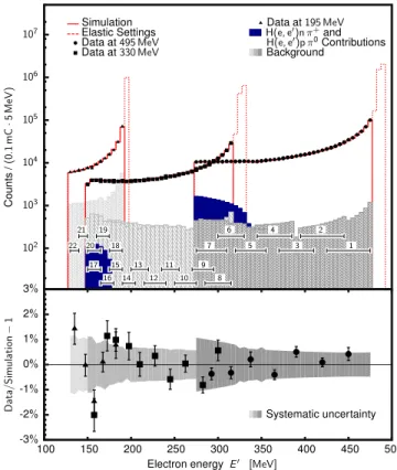
The ratio of measured and calculated cross sections shown in Fig. 2 (bottom) are in agreement to within a percent for all three energies. Considering the Bernauer fit [16] as a credible description of GpE this demonstrates
102 103 104 105 106 107 C ou nt s /( 0. 1 m C · 5 M eV ) -3% -2% -1% 0% 1% 2% 3% 100 150 200 250 300 350 400 450 500 D at a/ S im u la ti on − 1
Electron energy E′ [MeV]
Simulation Elastic Settings Data at 495 MeV Data at 330 MeV Data at 195 MeV H(e, e′)n π+and H(e, e′)p π0Contributions Background 1 2 3 4 5 6 7 8 9 10 11 12 13 14 15 16 17 18 19 20 21 22 Systematic uncertainty
FIG. 2. (Color on-line) Comparison of the data to the sim-ulation. Top: Circles, squares and triangles show the mea-sured distributions at 495 MeV, 330 MeV and 195 MeV, re-spectively, normalized to the accumulated charge of 0.1 mC. The elastic data (dashed line) are omitted from the analy-sis. The simulations with GpE, given by parameterization of Bernauer [16] are shown with red lines. The measurements at 495 MeV, 330 MeV, 195 MeV were divided into seven (1 − 7), ten (8 − 17) and five (18 − 22) energy bins, respectively, such that two neighboring settings overlap for a half of the en-ergy acceptance. The residual contributions of target walls, target frame, spectrometer entrance flange and cryogenic de-positions are shown with shaded areas. The full (blue) areas represent the contributions of the pion production processes. Bottom: Relative difference between the data and simula-tion. The points show the mean values for each kinematic point, while the error bars denote their statistical uncertain-ties. Gray bands demonstrate the systematic uncertainuncertain-ties.
for the first time that the electromagnetic processes, which give rise to the radiative tail are understood to a few parts per thousand, even at 200 MeV below the elas-tic line. This is an important finding for the electron-induced experiments, such as VCS [18], which require precise knowledge of the radiative corrections.
The remaining inconsistencies between the data and simulation could be due to the higher-order effects that are missing in the simulation or unresolved backgrounds. However, they could also be attributed to the difference between the true values of GpEand the model used in the simulation. Hence, the results presented in Fig. 2 may also be considered in reverse. Assuming that the
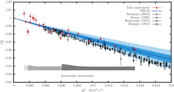
theo-Murphy (1974) Borkowski (1975) Simon (1980) Bernauer (2010) ISR fit This experiment Systematic uncertainty Q2 [GeV2/c2] G p E 0.02 0.018 0.016 0.014 0.012 0.01 0.008 0.006 0.004 0.002 0 1.02 1.01 1 0.99 0.98 0.97 0.96 0.95 0.94 0.93 0.92
FIG. 3. (Color on-line) The proton electric form factor as a function of Q2(= Q2Out). Empty black points show previous
data [19–22]. The results of this experiment are shown with full red circles. The error bars show statistical uncertainties. Gray structures at the bottom shows the systematic uncertainties for the three energy settings. The curve corresponds to a polynomial fit to the data defined by Eq. (2). The inner and the outer bands around the fit show its uncertainties, caused by the statistical and systematic uncertainties of the data, respectively.
retical description of radiative corrections is flawless and that background processes are well under control, the dif-ferences between data and simulation have been used to extract new values of the proton charge form factor. We have determined GpE for 0.001 ≤ Q2
≤ 0.017 GeV2/c2, thus significantly extending the low Q2-range of available data. The new values shown in Fig. 3 are consistent with results of previous measurements [19–22] in the region of overlap. The extracted new GpEvalues were compared to the polynomial G(Q2) = 1−r 2 pQ2 6 ¯h2 + a Q4 120 ¯h4 − b Q6 5040 ¯h6, (2) where parameters a = (2.59± 0.194) fm4and b = (29.8± 14.71) fm6, which determine the curvature of the fit, were taken from Ref. [23]. The three data sets were fit with a common parameter for the radius, rp, but with dif-ferent renormalisation factors, nE0, for each energy. In terms of this fit with 18 degrees of freedom and χ2 of 58.0, the normalisations and the radius were determined to be n195= 1.001± 0.002stat± 0.003syst, n330= 1.002± 0.001stat± 0.003syst, n495= 1.005± 0.003stat± 0.007syst, and rp= (0.810± 0.035stat± 0.074syst± 0.003∆a,∆b) fm. The reduced χ2 of 3.2 per degree of freedom (statistical uncertainties only) indicates that the results are domi-nated by systematic effects. Due to the limiting back-grounds and corresponding systematic uncertainties, we are unable to distinguish convincingly between the CO-DATA and the muonic hydrogen radii. However, we have proven the technique of initial state radiation to be a vi-able method for investigating the electromagnetic
struc-ture of the nucleon at extremely small Q2. This has moti-vated further experiments of its kind. Utilising a gaseous point-like jet target together with a redesigned spectrom-eter entrance flange will significantly reduce instrumen-tal backgrounds in the planned followup experiment [24] thereby extending GpE down to Q2
≈ 2 · 10−4GeV2/c2. The authors would like to thank the MAMI acceler-ator group for the excellent beam quality which made this experiment possible. This work is supported by the Federal State of Rhineland-Palatinate, by the Deutsche Forschungsgemeinschaft with the Collaborative Research Center 1044, by the Slovenian Research Agency under Grant Z1-7305 and U. S. Department of Energy under Award Number DE-FG02-96ER41003.
∗
merkel@kph.uni-mainz.de
[1] P. J. Mohr, D. B. Newell, and B. N. Taylor, Rev. Mod. Phys., 88, 035009 (2016).
[2] R. Pohl et al., Nature, 466, 213 (2010). [3] A. Antognini et al., Science, 339, 417 (2013).
[4] R. Pohl, R. Gilman, G. A. Miller, and K. Pachucki, Ann. Rev. Nucl. Part. Sci., 63, 175 (2013).
[5] C. E. Carlson, Prog. Part. Nucl. Phys., 82, 59 (2015). [6] A. B. Arbuzov, E. A. Kuraev, N. P. Merenkov, and
L. Trentadue, JHEP, 1998, 009 (1998).
[7] B. Aubert et al. (BABAR Collaboration), Phys. Rev. D, 69, 011103 (2004).
[8] M. Vanderhaeghen, J. M. Friedrich, D. Lhuillier, D. Marchand, L. Van Hoorebeke, and J. Van de Wiele, Phys. Rev. C, 62, 025501 (2000).
[9] L. C. Maximon and J. A. Tjon, Phys. Rev. C, 62, 054320 (2000).
[10] H. Arenh¨ovel and D. Drechsel, Nucl. Phys. A, 233, 153 (1974), ISSN 0375-9474.
[11] J. Roche et al., Phys. Rev. Lett., 85, 708 (2000). [12] L. W. Mo and Y. S. Tsai, Rev. Mod. Phys., 41, 205
(1969).
[13] Y.-S. Tsai, Phys. Rev., 122, 1898 (1961).
[14] K. Blomqvist et al., Nucl. Instr. and Meth. A, 403, 263 (1998), ISSN 0168-9002.
[15] M. Mihoviloviˇc et al., EPJ Web Conf., 72, 00017 (2014). [16] J. C. Bernauer et al., Phys. Rev. C, 90, 015206 (2014). [17] D. Drechsel, S. Kamalov, and L. Tiator, Eur. Phys. J.
A, 34, 69 (2007), ISSN 1434-6001.
[18] P. Janssens et al., Eur. Phys. J. A, 37, 1 (2008), ISSN
1434-6001.
[19] J. C. Bernauer et al., Phys. Rev. Lett., 105, 242001 (2010).
[20] G. Simon, C. Schmitt, F. Borkowski, and V. Walther, Nucl. Phys. A, 333, 381 (1980), ISSN 0375-9474. [21] J. J. Murphy, Y. M. Shin, and D. M. Skopik, Phys. Rev.
C, 9, 2125 (1974).
[22] F. Borkowski, P. Peuser, G. Simon, V. Walther, and R. Wendling, Nucl. Phys. A, 222, 269 (1974), ISSN 0375-9474.
[23] M. O. Distler, J. C. Bernauer, and T. Walcher, Phys. Lett. B, 696, 343 (2011), ISSN 0370-2693.
[24] H. Merkel (spokesperson), MAMI proposal A1/02-16 (2016).