3D turbine tip clearance flow redistribution due to gap variation

3D Turbine Tip Clearance Flow Redistribution due to Gap

Variation

by

Kai Yuen Eric Leung

B.Eng., Imperial College of Science, Technology and Medicine, London University

(1989)

Submitted to the Department of Aeronautics and Astronautics

in partial fulfillment of the requirements for the degree of

Master of Science in Aeronautics and Astronautics

at the

MASSACHUSETTS INSTITUTE OF TECHNOLOGY

June 1991

@

Massachusetts Institute of Technology 1991

Signature of Author.... ....

.... .... ...

. .. . ... ... .. ...

...

Department of Aeronautics and Astronautics

May 28, 1991

A

Certified by...

... ... ...

Prof. Manuel Martinez-Sanchez

Associate Professor, Gas Turbine Laboratory

a

Thesis Supervisor

Accepted by ...

. ..o.. ... .... ...

SProf.

Harold Y. Wachman

•~ m

i

hairman, Department Graduate Committee

3D Turbine Tip Clearance Flow Redistribution due to Gap Variation

by

Kai Yuen Eric Leung

Submitted to the Department of Aeronautics and Astronautics on May 28, 1991, in partial fulfillment of the

requirements for the degree of

Master of Science in Aeronautics and Astronautics

Abstract

The effects of blade-tip leakage in a turbine are investigated by modeling the stage as an incom-plete actuator disk. Taking advantage of the xz solutions for the spanwise flow redistribution due to constant geometrical gap width, they are generalized to include flow with some az-imuthal inlet velocity component which develops in the xy redistribution on the R scale when the turbine is eccentric.

The relevant flow quantities are linearized into their corresponding mean and perturbation parts. 5 downstream and 1 upstream perturbation modes are identified. Combining with the linear sensitivities calculated from the xz model, the coefficients for the perturbation modes su-perposition are calculated. The resulting perturbed flow quantities represent various responses of the downstream flowfield to a cyclically varying gap at the disk. Finally, the Alford force coefficients are calculated and correlate well with experimental data. Only the Alford force coefficient in the Y direction and the loss coefficient 1 are sensitive to changes in the mean geometrical gap.

Thesis Supervisor: Prof. Manuel Martinez-Sanchez Title: Associate Professor, Gas Turbine Laboratory

Acknowledgments

I wish to express my gratitude to Prof. M. Martinez-Sanchez for his guidance and instruction

throughout the project, not to mention especially his patience in going through all the details

of this work with me.

I am grateful to Dr. T. W. Poon and S. Yoo for their concern over my research work and

the progress in writing up this thesis. Much thanks are given to C. Adrian and A. Wong for

preparing the figures with me.

Finally, I would like to dedicate this thesis to my parents and my younger brother for their

love, care and prayerful support of me during this program.

Contents

Table of Contents ...

1 Introduction

2 Actuator Disk Theory for a Centered Turbine

3 Formulation 3.1 Linearization ... 3.2 Perturbation modes . . . . 3.2.1 a 3.2.2 a= - ... 3.2.3 a = - ... C+ 3.2.4 a = - . ...

3.2.5

aiR ...

3.2.6 Upstream perturbations . . . . 3.3 Linear sensitivities from the xz model . .

4 Solution to the Azimuthal Redistribution 4.1 Superposition of perturbation modes ... 4.2 Alford cross-force coefficients ...

Problem

•.. . . . .•

5 Some Results of the Linearized Perturbed Model 5.1 The nominal case ...

5.1.1 Spatialplots ... · · · · · · · · · · · · · · · · ... ...

5.1.2 Off-design operation ... .. 39 5.2 Various design conditions ... 40

6 Discussions

7 Conclusions and Summary

Bibliography Figures

Chapter 1

Introduction

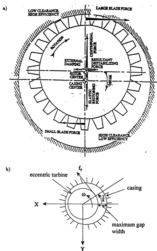
It has been known for some time that blade-tip losses of various kinds of turbomachinery generate de-stabilizing cross forces on turbine disks. These forces are only opposed by inertia and damping forces. The result, if damping is insufficient, is a divergent whirling motion. The loss factor P is important for the prediction of the stability properties of a turbine rotor. Fig.la) shows the contribution to whirl from turbine tip clearance effects.

Martinez-Sanchez and Gauthier [1] developed a theory to predict 3 from first principles, and to illuminate the effects of spanwise flow redistribution caused by the presence of a small rotor blade-tip gap. To this end, the blade-to-blade details were ignored by using an incom-plete actuator disk formulation which collapsed both stator and rotor to a plane, across which connecting conditions were imposed.

In their simplest version, the flow which leaked through the tip gap was assumed to do zero work. The results indicated that the flow tended to go preferentially through the gap, and that the attendant flux reduction elsewhere was very nearly uniform in the spanwise direction. The axial length scale for the flow redistribution was the blade height, and not the gap size. As a consequence, the unloading of the turbine blades was unifrom, and the work defect could not be localized in the near-gap region. The efficiency loss was found due to mixing effects downstream of the gap, between the bulk flow and the underturned and somewhat axially faster stream going through the gap.

Then, in their more sophisticated version, the underturned stream was recognized as orig-inating partly from gap flow, partly from entrained passage flow, both leaving the passage in

the form of a rolled-up tip vortex. The modified actuator disk theory allowed prediction of the fractional tip loading factor, and introduced the effects of loading level on individual blades, which the simpler version had ignored.

In this work, the same global nature of the blade-tip pattern is emphasized by using an actuator disk model for the stage. Provided one recognizes the discontinuous nature of the downstream velocity distribution (i.e. the presence of a shear layer along the tip streamsurface), the spanwise and the azimuthal rearrangement of the flow pattern due to preferential migration towards the gap region can be correctly captured. This shear layer is, of course, the result of azimuthally smearing the individual 'trailing vortices' of the blades. The xz solution of [1] then plays the role of a set of algebraic connecting conditons between the upstream and downstream flows. With some reasonable mathematical approximations, a generalization is made possible to include non-uniform gap distributions (our principal goal) and non-uniform inlet flow. The upstream flow redistributions which have been ignored in [1] are considered seriously here. Linearization of the relevant flow quantities by breaking them into their corresponding mean and perturbation part is employed as a major technique for the analysis. The results for the perturbation quantities will be directly used to calculate the Alford force coefficients which are the ultimate objectives of the whole work.

Chapter 2

Actuator Disk Theory for a

Centered Turbine

The model is that of [1] and will make the following assumptions: 1. Incompressible, inviscid flow

2. Two-dimensional geometry (x,z)

3. No variation along the tangential y direction

4. Fluid passing through the rotor-tip gap does no work

5. Stage collapsed in the axial direction to a single plane, and smeared in the azimuthal direction

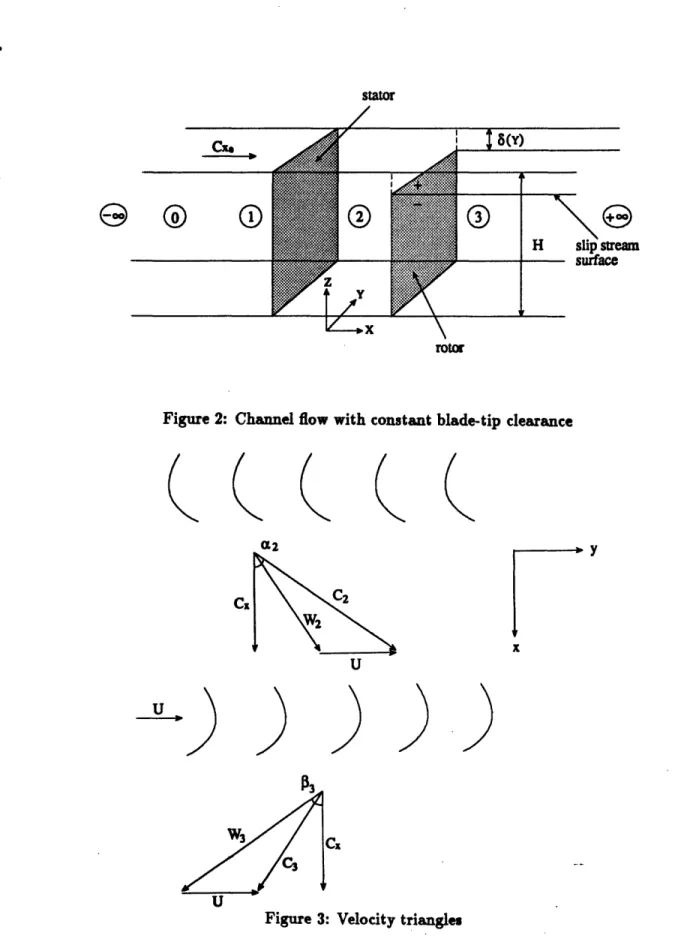
The 'actuator disk' which represents the stage consists of a full-span stator and a partial-span rotor (Fig.2), both occupying the x = 0 plane. The definition for BI of the meridional model is still valid here

B

= 1 (c2 + c2) (2.1)

P 2

Continuity is satisfied by introducing the streamfunction O(x,z) for the meridional flow:

a

?

c.- = - _(2.2)

c = _(2.3)

and then

cY = c

1

(o)

Wy = W,

(,)

BI = B(-)

where wOy = O _ V20 (2.4) SOz Oz

Notice that the meridional flow (c., c,) is decoupled from cy. cy1 = cy0, i.e. cy is purely

convected and does not change in the approach to the gap.

Upstream of the stage (x<O), the flow is assumed to be irrotational (wi = 0), and

b

simply obeys Laplace's equation. Uneven work extraction as the flow goes through the stage gives rise to non-zero vorticity wy downstream of the disk, and the value of wy is carried unchanged on each streamline from here on. It is further found [1] that

OB.

eW

=

(2.5)

This relationship opens the way for a connection between the downstream W• and the non-uniformity of extracted work at the disk. Let subscripts 1 and 3 denote stations just upstream and just downstream of the stage (Fig.3). Then because of continuity, and since spanwise uniform blading is assumed, which can exert no forces on the flow in the z direction,

cz3 = cz1 (2.6)

Because of Eq. 2.6 and the definition 2.1,

B - B = -P3 (2.7)

P

Now, upstream of the stage, the absence of vorticity implies a- = 0 and so from Eq. 2.5,

dB

d 3

B

1

- Bd

3 =

d

p

-

(2.8)

which gives the vorticity

oy

when the distribution of (isentropic) static enthapy extraction P--P

is known. The geometry of the stage blading is shown in Fig.3. Euler's equation gives for the stagnation enthalpy decrease across the stage

- Aht = U[c; tan a2 - (U - c- tan 0₃)] (2.9)

where U is the wheel speed. Adding to this the kinetic energy increase

A(K.E.) = 1 -

CO

) [(U - c; tan 13)2

-

c%0]

(2.10) we obtain, for any streamline which crosses the disk in the region covered by the blades (not the gap)

P - P Uc tana₂ - (U - c 2 tan 3) -~c (2.11)

As it has been mentioned before, no work is extracted from those streamlines which at some point cross the blade-tip gap. This implies for such streamlines

r - P3) p= - P = 1c+2 tan2 a 2 - - c (2.12)

P

P

= .2

2

In Eqs. 2.11 and 2.12, the axial velocities c+ and c- at the disk are to be regarded as functions of z, in anticipation of redistribution of the flow in response to the presence of the gap. When using Eq. 2.8, therefore,

d 0 (Oc, Oz (10 c~

dz ac, 8c . z /O,= C. 1~-z /,=o Oc,_

and so wy can be calculated from Eqs. 2.11 and 2.12 as

BLADES: w; = - tan a2 + tan2 33 (2.13)

(I

o=o

( 11)c=)

GAPS: w+ = - tan a2 --)= (2.14)

Since there is a discontinuity in the connecting conditions for flow through the gap versus flow through the blade passages, a discontinuity, in the form of a shear layer, is expected on

the downstream portion of the streamline which passes through the blade tips. Denoting by

superscripts

(+)

and

(-)

the regions on the gap and blade side of this layer respectively (Fig.3),

its strength (at least for the y component) will be

Q=jw

4I+ ,-B+-B;

(2.15)

With the help of Eqs. 2.7, 2.11 and 2.12, and the fact that no discontinuity exists in BI,

we obtain

Q

= Uc; tana2 - (U2 c-tan2 / 3)- 2 tan2 a2 (2.16)

Recapitulating, the equation for

4

is

upstream: V2 = 0 (2.17)

downstream: V

2 ₌

_tan

2

+

Q6(

-

t)(2.18)

- tanCa

+

tan2 / _8Z z _=o

- (c;).=o where 6(o - itip) is Dirac's delta function.

The boundary conditions are

(X, 0) = 0

;

/(a,H)

=

c.oH

C(-oo, z)

=

;

(+oo,)

=

0coz

0(0-,z)

=

0(0+,z) ; •(0-,z)

=

(0+, z)

Although there is some interest in the flow distributions elsewhere, the main results to the

obtained depend on how the flow is distributed at the disk itself. In the linearized approxi-mation in [1], the distribution is found to consist of two constant, but different axial velocity levels; one for flow crossing the gap, and the other one for flow through the bladed region. A general property of linearized, confined actuator disk flow is that the disturbance along a given streamline at the disk is half as strong as it is far downstream. This property accounts for the

factor of ½ in the following equations C+ Q = 1- + 2 (1 - A)...(gap) (2.19) CZo _2c 3,o

CC

Q

__ = 1 --

A.

(blades) (2.20) Co 02c,

where A is the fractional flow through the gap (namely, tip, = (1 - A)Hco). The quantity A is regarded as a given in our formulation, while the geometrical gap width 6 is not.

Substituting Eqs. 2.19 and 2.20 into the definition 2.16 of Q yields a quadratic equation for

Q

as a function of A. After some rearrangement, it becomes

(1 -A)2 tan2 a - A2 tan2 3 q2 + [2+(1 - A) tan2 a + tan a+ Atan'2 q

tana - + tan33 - tan' a

₂

]

= 0 (2.21)

where

4

is the flow coefficient

C- ₀

(2.22)

U

and the dimensionless shear layer strength is

q = 2- _(2.23)

The implied gap width 6 can be easily calculated as

6 A[1 (1 A)] (2.24)

H

2

This can also be solved for the leakage if the gap is given

A 27 (2.25)

1- + (1- )2+4 (Q )()

Notice that A depends non-linearly on r, both explicitly and through the dependence of q

on A (Eq. 2.21). For the practical, small values of A and

k

this is not a strong non-linearity, however.

The power extracted by the turbine, hence the tip loss coefficient, can also be calculated easily. In coefficient form,

9

=

U2

'

Ahtp

do

(2.26)

The total enthalpy drop is given by Eq. 2.9 for the bladed area, and is zero for the gap. Remembering that pm- = 1 - A, we obtain

P= (1 - A) (tan a2 + tan 3) - 1- A (tana2 + tanI33)]

For zero leakage, To = (tan a2 + tan, 3) - 1. The relative work defect is then

To 0 _ - 1 P+11- __ 1+ Aq11-A] (2.27)

I10

[

2

We can now calculate a work defect coefficient as the relative work decrease (Eq. 2.27) divided by the relative gap width

k.

Using Eq. 2.24,

w -+ -2 (2.28)

1--q

There is a hypothetical downstream section where the shear layer has dissipated and condi-tions are again uniform. At this 'mixed-out' downstream station, the axial velocity must again be c2o (to conserve mass) and the tangential velocity (from y momentum balance) must be

CymiM = Ac+ + (1 - A)c; (2.29) where c+ _{and c- and the tangential velocities in the fluid above and below the shear layer,}

respectively. From Fig.4, we have

c = c+ tan a2 (2.30)

cy = U -c; tan03s _(2.31)

where Eq. 2.30 reflects the assumption of zero turning of the gap flow, and Eq. 2.31 assumes perfect guidance by the rotor blades for the rest of the flow.

The total pressure in the mixed-out region is given by

Pto - Ptmi P - Poo 1 () (2.32)

p P 2

where p. is at a far downstream position, (before or after mixing) and we have taken advantage of c,. = cco, ca, = 0. The static pressure drop can be calculated for a streamline which goes through the blades. The drop p, - p3 at the disk, is given in Eq. 2.11. Upstream of the disk,

p - 1z= 1 c _(2.33)

P

2

2

and downstream, since c. remains invariant,

p- p3

1

2

2

1

2

P = (cz +C2)=0- c2 (2.34)

Here (c,2 )z=0 is a 2nd order quantity in our linear analysis, and will be ignored. Subtracting Eq. 2.34 from Eq. 2.33,

Po - Poo P - 3 1 2 1 2

p - p + c 2 C (2.35)

Combination of Eqs. 2.31, 2.34 and 2.11 therefore gives the total pressure change from far upstream to the hypothetical downstream mixed-out station. This quantity is the ideal work extracted per unit volume, and the efficiency is then

r = ' (2.36)

where 9 is as given by Eq. 2.27. The efficiency loss factor follows as

6P= (2.37)

As noted, the efficiency q is affected by the decrease of 9 due to the gap, but (see Eq. 2.35) also by that of the total pressure drop. With no gap, and everything else being ideal, q = 1. In general, 0 is smaller than w. Also, it has to be mentioned since the work done by the flow is uniquely related to the disk throughflow (c1).=o0 (see Eqs. 2.11 and 2.12), the implication is

that the turbine work defect due to the presence of the gap will be distributed uniformly along

the blade span, in correspondence with the uniform decrease of (c))=o0

Chapter 3

Formulation

In the previous analysis [1], the geometrical gap width 6 is constant. Here, the gap varies once per cycle along Oy (Fig.2). Hence, the approaching flow and the leaving flow will be affected over distances of order R, and will respond by redistributing in the xy plane. Now, at distance of order R, the xz redistribution due to the gap is not present yet (or anymore, for the fluid leaving ) because the flow shifts towards (or away from) the gap over distances of order H, as can be seen from the shape of the shearing streamline [1].

This means that, to a first approximation in -, the approaching flow can be taken to

be independent of z up to the disk, where it has already undergone rearrangement in the y direction, and the leaving flow can be taken to have a two-layer structure with the gap jet and the blade region flow being each independent of z. The xz solution of Chapter 1 then plays the role of a set of connecting conditions between the upstream and the downstream flows.

To take advantage of the xz solutions, they need to be generalized to include flow with some cY inlet component which may develop in the xy redistribution on the R. scale. However, once this is done, the xz and the xy problems are decoupled.

On the H scale, there is no pressure gradient in the y direction so cu₁ is the same for both the gap and the blades, having been induced far upstream on the R scale by the pressure gradient 2 due to the gap variation. Thus cy is purely convected and does not change in the

approach to the gap, resulting in c, = co.0 cYo will be used throughout the whole subsequent analysis.

The work defect coefficient w calculated for the xz centered turbine problem still applies at each y value when A = A(y), Q = Q(y). However, co must be reinterpreted (Eq. 2.22). Now, distances on the H _{scale but not the R one will be considered 'far', i.e. czo = c=o(y), 9 = O(9),}

as determined by the xy redistribution as z -- 0 on the R scale. For the downstream region, there are two layers which can be assumed to have the same p at a given point on the xy plane. Each of them conserves mass (no mixing) but their fractional depth may change.

The main analysis will be carried out by considering the continuity equations in the far downstream region,

O(Ac+)

(Ac+) -

0

(3.1)

+

= 0

(3.1)

Oz " y

0((H - A)c;) ₊

O((H

- A)c) _{= 0}

0

_(3.2)

(3.2) Ox ay

and the momentum equations

O(Ac+

2

₎

_(Ac+C)

_A

_0p

+ ₊ • 0 (3.3) ax 8y p Ox

O(Acc+)

O(Ac +2) A Op

+X Y + = 0 _(3.4) ax

ay

p 8y

8((H

- A)c;2)

O((H

- A)c+cy) 1 ap

+ + (H - A) - 0 (3.5) Ox Oy p Oz

a((H - A)cc)

8((H - d)c-

2 )

₁

_Op

((H- A)c;c)

+((H

-

+ (H

-

A)

0

(3.6)

Oz +y 8y p

Upstream of the disk (-x >> _{), the flow is taken to be irrotational and two-dimensional in the}

3.1

Linearization

With all the necessary flow quantities obtained, the next logical step will be to linearize them about a normalized mean gap -. This will produce a layer thickness A which will be the A(z - _{co) on the Hscale, namely, to the 1st order in the disturbances,}

(1 - (1 - )) (3.7)

Since

A is a far downstream quantity, it can be noted that the q term is doubled when compared

to Eq. 2.24. Splitting the flow quantities into their corresponding mean values, which are from the xz solution at 6 = T, calculated at x > , and the perturbation parts, gives

A = A+

'

(3.8)

C+ =

+

+ 'C (3.9)

c+

= + + +•

(3.10)

cg = c + c' (3.11) cy = C +c' (3.12) p = p+i (3.13)

But now the far upstream co becomes

c=0(Z, y) = C-- + c~0o'(, y) (3.14)

where U0 = c,_-. = constant.

Taking the mean values on the gap side at the disk (x > ),

=

1+ c(1-..X)

S1+(-

)

(3.15)

CaO

C,0

(CV)B=O-CO0

= tan a₂ (1 +

₂

(1 -))

similarly for the blades side,

= 1-q.

U

C-'O

-

tan/3a

(1

All the ( ) quantities are constant. For the ( )' ones,

LJ'=3[ri

where ( ) _{is a function of x only, and R denotes the real part of}

Eqs. 3.1 to 3.6, the downstream flow (x > H) is governed by

a complex number. From

d

(,&

c

4-

+

_XL -,

)+

d

((H - A) cc - cA)

- dc ct l

_dz

dc;

_dz

dc

R

Y

+

)

+•

+

+

1 d,6

Sp de: i P v - i - 1 dp

+ c~7

-

c

+

R p dz (3.16) (3.17) (3.18) exp i = 0 = 0 = 0 = 0 = 0 - 0 (3.19) (3.20) (3.21) (3.22) (3.23) (3.24) -

Ri-+ c; _y 1 i pR

+ ((

-Y - a

+ + c

R+

Now treat () = ()exp(az) and the () quantities are complex constants, and a is an axial wavenumber to be determined for each mode. Eqs. 3.19 to 3.24 can be written in matrix form

aA

0 0 0 0 0

act

₊

_CY

0 0 0

a(H- A)

0 0 ac + Xc; 0 0 S(H - A) 0 0 0 ac + *c act + + + -ac - c 0 0 0 0 0 0 a a oS c. cc A =0

(3.25)

For non-trivial solution of the column vector containing all the relevant ( ) quantities, the matrix constructed is singular, i.e. its determinant is equal to zero. This leads to the charac-teristic equation

i -:) - s-i 1

act

+

-

-) a'

+ (H - )a

0

(3.26)

The six roots of the polynomial equation correspond to six different downstream perturbation modes which will be discussed in the next section.

The geometrical gap width is described as

(3.27)

= e' R exp iI

where both w, e' are real constants. The second term is the perturbation part of ( and is

used as a reference for the phase shifts of all the perturbation quantities considered above, since the whole idea is to see how those quantities respond to a cyclically varying gap at the disk. It is not necessary to know the value of e' as the variable can be readily used as a normalizing factor. However, -M must be specified for the calculations of the mean flow quantities.

3.2

Perturbation modes

The six roots of Eq. 3.26 are

cz

c,

and

Anc.c;±+(H-A)c,+T+±iVA(H-) IC;-c Ci

iRa =2

-Ac; + (H - A) ct

With the roots known, the perturbation modes can be worked out correspondingly.

3.2.1

a-=1

This represents divergence of the perturbations far downstream of the flow leaving the disk. It will be disregarded. Then, there remain five downstream modes to be considered. Since the stage itself has an influence on the upstream flow at the far upstream station, an upstream mode will be taken into account, as will be discussed later.

3.2.2 a = -1

This represents convergent potential effects, i.e. effects in this mode will die out with x, down-stream. From the momentum equations 3.21 to 3.24, and substituting for a,

(-c, + ic•) C

+

_p

=

0

(-c+ + icy ) C+

+ i

-

=0

P

(-c; + icy) c;- -

= 0

S -CT +i CY -1

-cc +i

Ct

and from the continuity equation 3.19,

-9

P -c; +i c

By substituting the corresponding ( ) expressions into the above equations,

(-c

+

+ ic

+

) A

=

0

= A = 0 in this mode

The zero condition is also satisfied for the continuity equation 3.20 as all terms are cancelled out. Writing the results in vector form,

c+'

C,

c+'

c

Y

11' A' p. =

R

1

-ct

+

_i

+ -C-+i4y -i

-co +icy

-i

1

pexp

( + -)

P (-W

(3.28) 3.2.3 a = -- L

This represents the convective mode in the blades region, i.e. the (-) side of the dividing stream-surface. Rearranging the root expression,

Substituting this into the (-) momentum equations in 3.25, it is found that = 0 in this0 mode. Then from the (+) momentum equations, ce = c= = 0. = 0A 0 is obtained from the

(+)

continuity equation while the (-) one gives

Cy a

•

Again, the results can be written in vector form

c+

C2 c•' a

c

P -R 0 0 1

0

CYr c.

exp

-R

c-

(3.29)

This mode contains only the perturbations aligned in the c- vector direction but no other ones.

c+

3.2.4 a

-This root is similar in nature to the one in subsection 3.2.3 except it stands for the blade tip gap region, the (+) side,

c+'

c+' c; C-c-' -R 1 0 0 .' I (3.30)

This mode contains only the perturbations aligned in the c+ vector direction but no other ones.

r

· I \

· /

ct exp

_R

y- s

c-3.2.5

aiR

Ac. cj

HA);

+ ((H -

c+ca

A

))

T.

Ac;

+ (H -A) c

2

The last two modes represent slowly decaying and growing effects downstream respectively. The latter is thought to be the Kelvin-Helmholz shear instability. Dropping only the (-) continuity equation of Eq. 3.25, the rest become

A (aiR)c. - Ac + ((aiR)ct -

c,+),A

= 0 (3.31)

((aiR)c+ - c+)c4 + (aiR)

-

_P

= 0

(3.32)

((aiR)c,- -

)c4-

_P

= 0

(3.33)

((aiR)c - cy)c; + (aiR)

-

= 0

(3.34)

P

((aiR)c; - cy)cY - - = 0 (3.35)

Eqs. 3.32 to 3.35 are rewritten as expressions of the () quantities divided by 9

+ +

S

(ai)

c+

-c

+Y 1

(caiR) cM -Cy

Here,

A«H, ai4R ~4 i

T

- (3.36)

+ HHai+R " ++

Substituting the roots 3.36 into the above

c

gives an expression for P. The corresponding vectors are P +c Cg_+' Cu I -I A' 4. K (3.37) The two modes, one decaying and the other growing, are simultaneously convected essentially with the c- vector, having wavelength 2'rR. The damping rate is proportional to the absolute difference between the tangents of the two flow directions relative to the axial direction. For modes 1, 4, 5 and the discarded one,

B' = 1 (c2, + C 2)' + --c' + -' + B+ = cc +cTc

+

=

0

similarly, B- = 0. For mode 2, c = = = 0 B+ = 0

i

r/ Cz

4~

C; c c- 2-2 1+

S

_{cc + cY}

cTYc

r

I

- exp

-C

y

+

T C

p R

R H

c

exp~ Y-c

~~F

] H C T X+

4 5

9 I , I

and

=~ c, + cfl Cf +

~-

_P

=

-c_

+

c C

+

c;

2 C;

(c)

-cc

For mode 3, c? = Cy = P

=0

0 B-=O

and

B+

(c+) 21.

So modes 4 and 5 which convect shear (and vorticity w,) also convect total kinetic energy, but all the others are iso-energetic.

3.2.6 Upstream perturbations

c, _, is a constant but by the time when the flow reaches the far upstream station (H < <

R), c, will have deviated from its original course. Thus,

cXo =

c-oo

+

C'o(y)

(3.38) A streamfunction ((x,y) is defined in a similar manner to that used in Eqs. 2.2 to 2.4, (x

c

(Z,

y)

c,((,

y)

(3.39) (3.40)

At distances on the R scale far upstream,

(3.41)

a~E

Bernoulli's equation is also obeyed, Po + 1 c,(z = 0-) + cY(Z = 0-) 2 -" + 1 ci2 P 2 2 p0 perturbing gives - + c,_,₀c',( = 0-) + C_ ( = 0) = 0 (3.42) P

Seek a solution for f in the form ( = exp (i

(+

+ az)) where i is a costant. Substituting this solution into Eq. 3.41 yields the two roots a = - .

Therefore,

e

= (exp(i(

+az))

(3.43)

C =RexP i(

+a)

(3.44) - Yexp (3.45) y

_11.

ly

-1 ₊ =-- ~- [-ic_.- + c_,] exp i + (3.46)

where the real part of the complex right hand sides is implied.

In the upstream region, x < 0 so only the non-amplifying root is kept. In the upstream region, at the disk (x=O-) we then have

c'(z = 0-) O iKoexpi (3.47)

c(z= 0-) = -Ko exp (i)

(3.48)

where Ko =

Altogether six modes are identified for the perturbation quantities. Once the ( ) quantities are solved as coefficients for their corresponding modes, the whole perturbation flowfield can be calculated.

3.3

Linear sensitivities from the xz model

In order to calculate the coefficients for the perturbation modes, q and A must be known in the first place before all the downstream flow variables can be calculated. },

4

and ?7 are identified as the independent variables, i.e.

= ( , , )...etc.

A

= V

First of all, q and A are iterated by using Eqs. 2.21 and 2.25. Then 9 (Eq. 2.27), + (Eqs. 3,15 and 2.22), - (Eqs. 3.17 and 2.22),

s

(Eqs. 3.16 and 2.22), and - (Eqs. 3.18

and 2.22) can be calculated. From continuity,

•A 1+ P( - )

=

+

2

_(3.49)

H H 1 + q(1- )(3.49)

Now it is necessary to calculate the first order sensitivities of these variables on , and 5F. Partial differentiating Eq. 2.25 w.r.t. q and r respectively and evaluating the derivatives at

the azimuthal mean values, gives

=OA1-•

746

(3.50)

(

=2A

q 6

(3.51)

can be done by partial differentiating Eq. 2.21 w.r.t. A and • respectively,

(() =

tan2

2a2+

ta

q

+

tan2 a2 - - tan2

33

(I-X)2 t=n2 a2-X2 tans _{- s tn} 83

+"

₊

₂

₊

_{(1- ) tan2a •anaz 2 +}

₊

_{· tan2 /3}

x( q

%tana 2 + (- tan a)

(1-X)= tan2 a2-n -X2tan s + tan

4 + 2 + ( 1 - A) t an 2 +

tana2

+ A tan

2

3

3

Also,

q

= 1-(1- 2A)

(=~X

-

-72

In Eq. 2.21, q = q(A, 0),

= (-) * d) + (4)dd

Thus,

ex rq

1 _

(3.56)

(3.57)

(3.58)

BkI 68 q + go \ IAj

q (3.52)

(3.53)

(3.54)

(3.55)

\BII

1

(3.59)

Now, all the basic flow sensitivities are obtained for calculating the flow velocity and pressure sensitivities to 6, and IL. Far downstream (x> H), the c., velocities are

=

[1+ q(1-

A)]

= 0(1 - qA)

=

_ (1

(- ),(-•

)

=

[1 + (-)]

(a)

)

(3.60) (3.61) (3.62) (3.63) (3.64) (3.65)

There are also four sensitivities like Eqs. 3.60 to 3.65 for c . Only c- in the vicinity of the disk are considered, for reasons mentioned in the last two chapters. Hence, there is a factor of I in the q term in the following equations

C₁₁

U

c;

U

(+)_a81 ali ,

#/

oTi ]₄,

= tana2 1

+

!(1

-

A)

=- _{1•tan3 [1}

-tana2[

₂

₆

+

11

tana33 (3.66) (3.67) (3.68) (3.69) (3.70) c0oo

U

C00

U

q +

q

Ir

By using Eq. 3.49, it can be calculated that A

2

+

(1

+

q(1

-

A))

2

2 + (1+ q(1 - ))

2 From Eqs. 2.11, 2.22, 2.35 and 3.61,

= tana2 ( 1

-2

Thus, the corresponding sensitivities are

[-a

ig

r1

(

~)L

I

_-

C-1

-i

+

2 tan

2

p3

(

1-1

2

tan a2 - 2 tan3 1 (3.75)

q

+

tan a2 - 22 tan2 P3

2

2) 2

-

4

1

2

tan

a

2

+

- 1]

Notice that

e

_{is the only quantity which depends on 5P.} All these flow velocity and pressure sensitivities to 1,

4

and W for the nominal case are shown in Figs. 7 a)-m).

tan P3 2

+i]

(;~)

(3.71)

[(1

(3.72) (3.73) 2

(3.74)

-

2

-2)

2

2-tan2 / 3

La

(PO

-P)r

(3.76)

(3.77) -Q eex,,1_,15

AO-

)

q(

_@W)

ax

₆

+ 61

Chapter 4

Solution to the Azimuthal

Redistribution Problem

4.1

Superposition of perturbation modes

The downstream mode vectors identified in Section 3.2 can be rewritten in a generalized sum-mation form 5 ct = Ki(c ), (4.1) i=1 5 c = - Ki(c ) (4.2) i=l 5 c =

Ki(c;•)

(4.3) i=l 5 C = ZKi(C )i (4.4) i=1 5

S=

Z

Ki(A)i

(4.5)

i=l

=

K,()

(4.6)

P Pi=1

where Ki (i = 1,..., 5) are complex coefficients. They are considered at x=O, and are virtually equivalent to the () quantities in Eqs. 3.28 to 3.36 with the exp (i Y) term dropped. Eqs. 3.28

to 3.30 and 3.37 can be written as

c .

A

cA

c;

CY ,,,,. cz where s+ = 1 + + -i

0+

1

!L

c, +K2

0

CY _ I

0

+K3

cW

0

0

0

0

The other way of writing Eq. 4.7 is

cc

C; cc CY P = C(x = 0-)U

U

o

+

y(a = 0-)

U

_

0

8

Equating Eqs. 4.7 and 4.8 and noting Eqs. 3.47 and 3.48, six equations are obtained,

( )

8-5&

EKi(-)

5 2=1 i=1

ZKi(c-)i

-c+ Kog

-C

(

KoT

i

6Ko

(

7;

+

R

Ko

=

e'

IT

~

T

= el = el = e' = He' K( Ko2H= i= 1 y -s+sg

sg

H --+ 2

c,

Is+

-

-

I

18+2

-i9/

c; Is

+

-

s,-I

(4.7)

C+

c o

c-A PO-PoC (4.8)

(4.9)

(4.10)

(4.11)

(4.12)

(4.13)

I -. m sg =- i _I.

+ el 8

5

K=1 p

+

_·[~d~e~~7y,

(&)6UKio-

A$

_F

+

₄

UKo

0

74

(

)

I ,1I

=

-u

2

[ a(e'

(4.14)

The system of equations is then solved by Gauss elimination for the Ki's (i = 0, 1,..., 5),

/

C7)

-

I + isg(1 + as+s )

(7/)+

(~j~

o4)4

,

ra - /

r

- \ cq 6 CU

J

UTI

[Is

+ --

I

+ isg (1 + S+s-)]

Ue'

_7;

6

1.+ - - -1 + s+2

I1 -

s-I

1+ 9+2

K4 + Ks

Ue'

+

{

1 V

iUe

-

1Ue'

K2

1

ji

_{K4 + Ks}

Ue'

Ko

Uel

Car

U

if

T8

-2 2-UC;

K

₄

+ Ks

Ue'

K

₁

U2e'

U c_

=---i-(4.15) (4.16)

K4 - Ks

Ue'

[ ( )

(

9

r

_1015f

_ýi~

(4.17)

)0

UY,

U

K

1

U

2

_e'

(4.18)

+i

-4 +

K2

e'

-)2

C--

+

U e

+ .9+2[1

-I

I

=

(

)i .

4

L~·r \ rV /JR~tr latfL \ ''- /1 a

Cl

A

4ý

.( 817 )0

7F

1

6,

-i

( )1

Ko

q a°

17 ) A,

+iKo

(4.19)

K

3

1(

+

H K2

- Ks

e'

e

+

V'

Ue'

+i) (4.20)

Due to the relationship between modes 4 and 5, there is no need to work out K4andKs indi-vidually. The whole flowfield is basically solved at this point giving the perturbation vector divided by Ue'.

4.2

Alford cross-force coefficients

Writing in terms of the force f per unit azimuthal length

f

= p ]

(c;2 -

C 3

)do

(4.21)

Remembering that O/tip = c.oH(1 - A), and that, according to Chapter 2, cy is uniform in &,

fy = P(c;2 - c•3)c,oH(1 - A) (4.22)

Perturbing gives

u = pH[-(c;2 - cY3)A' + (c42 - c 3)(1 -

X)eC

0 + O(1' - )( - )] (4.23)

The total cross-forces in the horizontal OX and the vertical OY directions can now be calcu-lated by projecting

f,

in the two directions respectively,

F = 2.Rf , sin Rdy (4.24)

Considering the algebra involved,

()'

₌

_[()exp

_(i) exp (i

(

)'sin

Idy

o R 2iR

..d

Jo

eo COS dR

=

I(

)1 cosOco

= -rRsinOl( )

= -?rR ()

=

rRcosO•()

- rRR(

O

+ Y

(R+

i))]

y

~y\

R - sin O sin-R

R

R

where 0 is the phase angle of the ( ) complex number.

Therefore,

quantities. ! denotes taking the imaginary part of a

Fx = -pHrR . [-(cY2 - cY )A + (cY, - c,3)(1 -

.)c-+c-(1 - )(c;Z - CY 3)]

Fy

= -pHrRR[-(c;2 -CY)O+ (cy2 C )A-lC - C

+

(1 -

)(c,2

-

c;V)]

Define the Alford cross-force coefficient

2FyR

ay

Q el

Fy

7rR e'

R[-(H

2 - CY

)A

+ (C -Cy 3)(1 -

)o +

C-(1 e - e'1-=

p(c;

- c; ) c•H(1 - X) (4.26) (4.27) (4.28) , C -- C1 C-O - CY3

C,0

_{CY 2 - CY 3}

(4.29) (4.30)

- A)XCY - cy 3)]

=r 0

where

_fh

ay is positive for forward whirling force.

Similarly, defining ax =-

2

gives

ax

e'

_{W - A cr o}

-=

cy

~

-

Cy

C 2 - c; 3

(4.31)

ax is positive when the cross-force is de-stabilizing but will be negative if it is due to spring

action.

Chapter 5

Some Results of the Linearized

Perturbed Model

This chapter gives some simple calculated results from the formulae obtained so far, in order to illustrate the trends and sensitivities involved.

As it might be expected, the degree of reaction R is an important parameter controlling the effects of tip leakage. At very high R, the turbine is lightly loaded and the effect of the gap is small. This can be seen most easily in the zero exit swirl case (design point),

1

(5.1)

tan 33

R = 1 tan a2 (5.2)

tan

/3

indicating I = 2(1 - R), so that 9 --+ 0 when R -- + 1. At the other, and more realistic end (small R), the individual turbine blades are highly loaded, but there is little net pressure drop across the rotor. Since there is then little incentive for approaching flow to migrate spanwise towards the gap region, little blade unloading is expected.

Two categories of plots are produced: a) Spatial variations of various quantities for a par-ticular operating condition, and b) magnitude and phase of various flow quantities vs. mean flow coefficient ý. For both plots, the basic parameters Rdesign, gap=0, hdesign, gap=0 are specified, and then using Eqs. 5.1 and 5.2, tana 2 and tan/3 are calculated accordingly. The average gap j values have been selected as 0.008, 0.016 and 0.028, which are considered in

both catergories of plots.

5.1

The nominal case

Rdesign, gap=0 = 0.206, 4design, gap=0 = 0.58

5.1.1 Spatial plots

A particular ýselect value is chosen for the plots and should be distinguished from

Odesign, gap=0. In the this case, it is taken as select=0.5 76 . The flow quantities e, ,

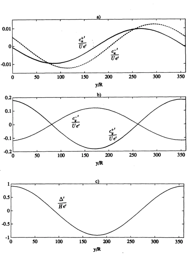
, P,, atr --- ), (o-) _{are then plotted against $ in degrees (Figs. 4 a)} -e)). The

range of 's considered represents one cycle of variation of the geometrical gap V. Wr is totally in phase with and should be used as a reference curve for the phase shifts of the rest. Both eandT have phase lags of about 900 with the former lagging more. The amplitude

_+1

of YL7 is substantially larger than that of .

Iis

almost in phase while c is almost totally in counterphase. Their order of magnitude is 10- , much larger than that of + , which is 10-2.

- and -P are also almost totally in counterphase. The downstream static pressure perturbation is expected to be smaller than the one between the stators and the rotors since

work is being extracted from the turbine.

The upstream perturbations Uoand,4( ) have the same amplitude of about 0.14

but the latter lags behind the former by 900. '.(=0-) is in phase with 6' (maximum axial

flow where the gap is maximum, as expected). This explains the fact that p'2 is minimum at maximum gap. The order of magnitude is about the same as that of -.

5.1.2 Off-design operation

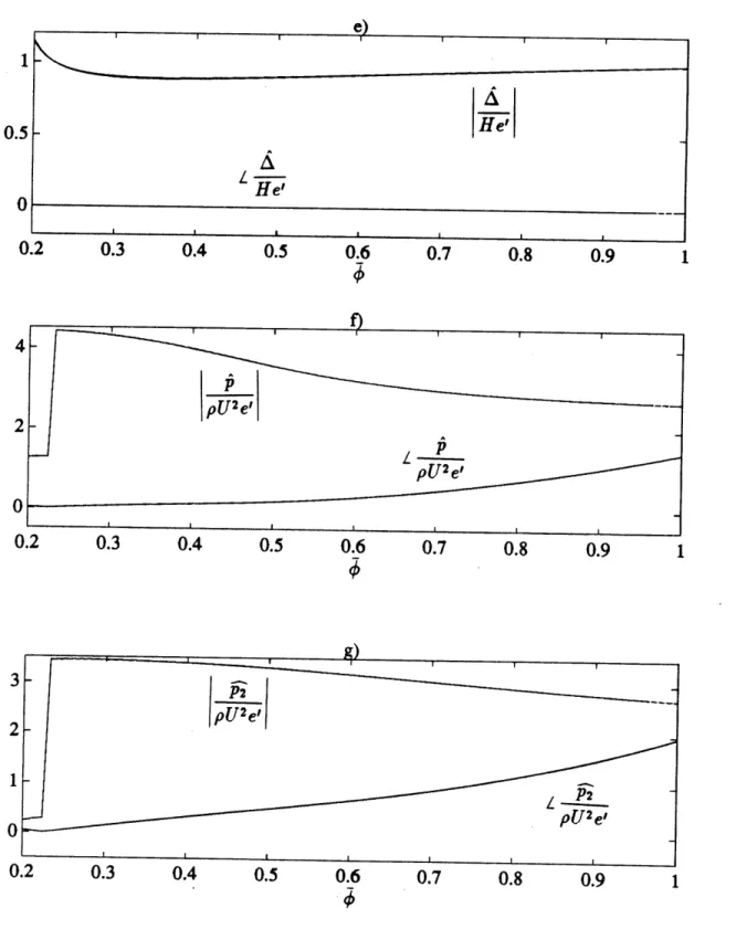
Keeping the same a2 and p3 and using the same set of 4 values, the magnitude and phase of

,

,

pe"

-~

,

o

e'

o-), 4t

and

4

_{are plotted against •. • ranges from 0.2}

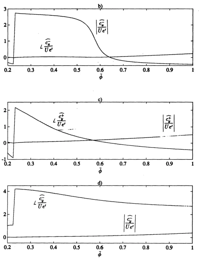
to 1.0. The Alford force coefficients ay and ax are also plotted against •. Singularities occur at the idling point at

4

_ 0.22 for most of the flow quantities except that iv which shows a maximum there.

Both i and 1 turn almost 1800 when ý is increased from the idling point to ý=1.0. The drastic change in phase occurs roughly at kdesign, gap=0 where their magnitudes are minimum. Thereafter, they increase with 4.

The turning of ; with ý is also large but • has a phase change of only about 900 over the range of ý considered, while both of their magnitudes increase monotonically.

and

behave similarly to

with

.

9 has a minimum smaller than unity at ~c 0.36. At the idling point, it has the value of 1, and is expected since when the turbine is not producing any work, the flow through the gap will have no difference from that through the blades passage. Then, A = 7 = e'. The phase is zero for all values of • considered.

Both ,( 0-) and

•4

-) increase with ý. The turnings are only about 450. The order of magnitude is 10-1. The gradients of the phase curves near the idling tend to zero indicating

the upstream perturbations are not sensitive to changes of ý if the turbine is idling.

5.2

Various design conditions

Other than the nominal case, 4 more cases with different combinations of Rd,,. and &d,,. are ex-amined. The Rdea. values are 0.0 and 0.5 while the 4

des. ones are 0.3, 0.6 and 0.8. As it has been seen in the nominal case that too many variables are involved, only

Pj',,

t ay, ax, and ti

are considered. There are no significant differences in the general trends from the nominal case. By changing kde., the behavior of the flow quantities of interest at either the high or the low end of the ý spectrum can be viewed. Singularities occur at low 0 for the pressure perturbations when des. is high, irrespective of R&,.. Again, $ has an effect on / only.

Chapter 6

Discussion

In the downstream region, the flow totally redistributes itself. The flow perturbation quantities which lag behind the gap by about 900 almost vanish at maximum gap indicating the through-flow there consists of only the mean part. Whenever work is extracted from the turbine, the azimuthal flow perturbation cy is approximately in counterphase with the gap distribution. This also happens to the two pressure perturbation quantities considered and has already been explained in the last chapter. The xy redistribution starts upstream when the flow sees the effect of the eccentric turbine. It has been noted that the azimuthal flow perturbations do not change when they are convected downstream.

Variations of various flow peturbation quantities for the nominal case, in terms of their phases and magnitudes are shown in Figs.5a)-k). Most features have already been pointed out in the last chapter. In general, the magnitudes increase with the mean flow coefficient. One of the exceptional cases is A which first decreases and then increases to unity with ý. Closely examining the minimum point shows that it coincides with the ones of the sensitivities, indicating its general trend depends strongly on how sensitive the flow quantities are to the mean flow coefficient and the mean gap value. However, as it has been noticed before, the mean gap variation does not alter the results at all, even when the value is increased more than

three-fold.

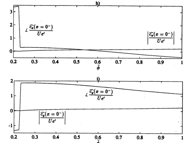
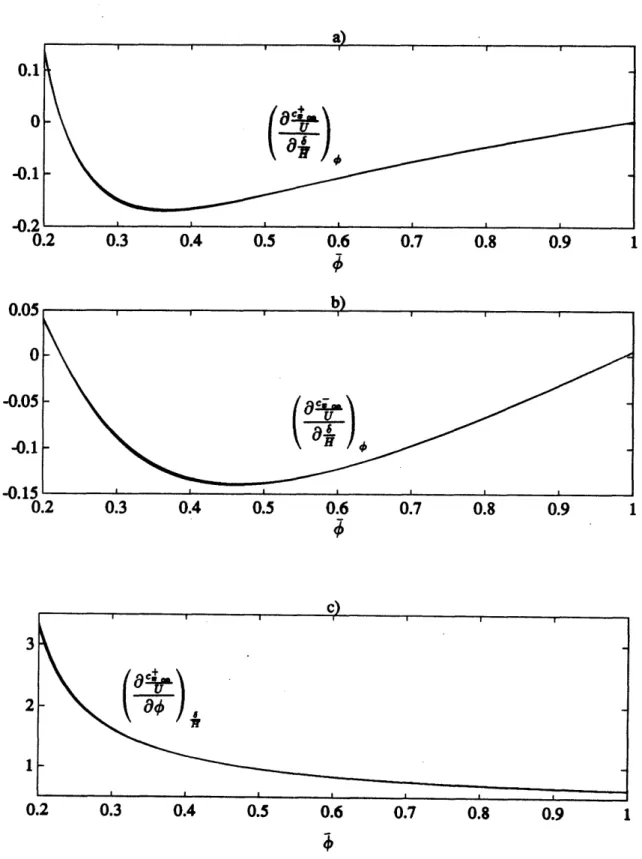
There is a minimum value near the design point for each of the axial flow perturbations. This is a feature which is not expected. It can be visualized as a velocity vector originating from the origin moving along a locus which is very close to the origin itself. The nearer does

it get to the origin, the smaller the magnitude is but at the same time, the phase is changing continuously. Eventually, it happens to have turned 1800. So, near the design point, it will have an important consequence to setting-up an experiment in the effort of measuring the axial perturbations. It would imply that a turbine test set-up has to be run in off-design conditions in order to measure the c±' redistribution. c'~(z = 0-) is non-uniform in the upstream region but after the flow has passed the disk, the downstream axial velocity perturbations become uniform instead. The mechanism in which it happens is not too well understood and is to be found out in due efforts.

ay decreases while ax increases with

4.

Experimental values show that at the design point,

ay is bigger than unity but the analysis shows it is less. ax is found to be zero at the design

point. Experiments show that the latter is non-zero. The trends of it and

4

agree well with [1]. With zero exit swirl geometry, these two values do not alter much in trends when the geometry is changed by varying R,.. and 4_{dea.. However, the magnitudes of the pressure perturbation}

increase enormously when R&d. = 0.0 and seem to be suppressed if 1des. is increased, i.e. the

relative flow leaving the rotors is turned less. The Alford cross-force coefficients seem to be very insensitive to geometry changes.

Chapter 7

Conclusions and Summary

The effects of the blade-tip leakage in a turbine are investigated by modelling the stage as an incomplete actuator disk. The xy redistribution of the downstream flowfield from the disk is then developed.

5 downstream and 1 upstream perturbation modes are identified. Using superpositon tech-niques, all the relevant flow quantities are calculated. They are important variables for even-tually calculating the Alford cross-force coefficients.

The results are mostly reasonable and can be physically understood. The remaining mystery is the almost zero magnitudes of the downstream axial flow perturbations when the turbine is operating at the design point. The mechanism of the change of these perturbations from non-uniformity in the upstream region to non-uniformity in the downstream region is also yet to be found out.

The Alford cross-force coefficients are found to be not too sensitive to the change in the stage geometry.

Since the steady state solutions have largely been worked out, compressibility and unsteady flow effects can be included in any future work as the continuation of this research.

Bibliography

[1] M. Martinez-Sanchez and R. P. Gauthier. Blade Scale Effects of Tip Leakage. Gas Turbine Laboratory Report no.202, MIT, October 1990.

[2] J. H. Horlocks. Actuator Disk Theory. McGraw-Hill Inc., 1978.

[3] H. Cohen, G. F. C. Rogers and H. I. H. Saravanamuttoo. Gas Turbine Theory. 3rd edition, Longman Group UK Limited, 1987.

[4] A. J. Crook. Numerical Investigation of Endwall/Casing Treatment Flow Pheonomena. Gas Turbine Laboratory Report no.200, MIT, December 1989.

[5] N. K. W. Lee. Effects of Compressor Endwall Suction and Blowing on Stability

LZGlt~EBADgp OatCe

eccen

casing

num gap

Figure 1: a) Contribution to whirl from turbine tip clearance effects, b) Alford cross-forces notation

stator

rotor

Figure 2: Channel flow with constant blade-tip clearance

U

Figure 3: Velocity triangles

0.01

0

-0.01

0

50

100

150

200

250

300

350

y/R

0.

0.

-0.

_-0 50 100 150 200 250 300 350

y/R

1

0.5

0

-0.5

-1

0

50

100

150

200

250

300

350

y/R

Figure 4: Downstream perturbations of a) axial velocities, b) azimuthal velocities, and c) layer

thickness vs. y/iR

0.5

0

-0.5

0

0.1

-0.1

50

100

150

200

250

300

350

y/R

0

50

100

150

200

250

300

350

y/R

Figure 4: d) Static pressures perturbations, and e) Upstream velocity perturbations vs. y/R

0.2

0.3

0.4

0.5

0.6

0.7

0.8

0.9

Figure 5: a) Variation of downstream gap axial velocity perturbations with mean flow coefficient

for a fixed gemeotry

2

1

0

0.2

0.3

0.4

0.5

0.6

0.7

0.8

0.9

1

2

1

0

-1

0.2

0.3

0.4

0.5

0.6

0.7

0.8

0.9

1

4

2

0

0.2

0.3

0.4

0.5

0.6

0.7

0.8

0.9

Figure 5: Variation of downstream b) gap azimuthal, c) blade passage axial, and d) blade

passage azimuthal velocity perturbations with mean flow coefficient for a fixed geometry