Investigation of Atmospheric Turbidity at Ghadaa (Algeria) Using Both Ground Solar Irradiance Measurements and Space Data

(1)

HAL Id: insu-02112660

https://hal-insu.archives-ouvertes.fr/insu-02112660

Submitted on 26 Apr 2019

HAL is a multi-disciplinary open access

archive for the deposit and dissemination of

sci-entific research documents, whether they are

pub-lished or not. The documents may come from

teaching and research institutions in France or

abroad, or from public or private research centers.

L’archive ouverte pluridisciplinaire HAL, est

destinée au dépôt et à la diffusion de documents

scientifiques de niveau recherche, publiés ou non,

émanant des établissements d’enseignement et de

recherche français ou étrangers, des laboratoires

publics ou privés.

(Algeria) Using Both Ground Solar Irradiance

Measurements and Space Data

Djelloul Djafer, Abdanour Irbah, Philippe Keckhut, Mohamed Zaiani,

Mustapha Meftah

To cite this version:

Djelloul Djafer, Abdanour Irbah, Philippe Keckhut, Mohamed Zaiani, Mustapha Meftah.

Investiga-tion of Atmospheric Turbidity at Ghadaa (Algeria) Using Both Ground Solar Irradiance Measurements

and Space Data. Atmospheric and Climate Sciences, Scientific Research Publishing, 2019, 09 (01),

pp.114-134. �10.4236/acs.2019.91008�. �insu-02112660�

(2)

ISSN Online: 2160-0422 ISSN Print: 2160-0414

DOI: 10.4236/acs.2019.91008 Jan. 8, 2019 114 Atmospheric and Climate Sciences

Investigation of Atmospheric Turbidity at

Ghadaa (Algeria) Using Both Ground Solar

Irradiance Measurements and Space Data

Djafer Djelloul

1*

_{, Irbah Abdanour}

2

_{, Keckhut Philippe}

2

_{, Zaiani Mohamed}

1

_{, Meftah Mustapha}

2

1_{Unité de Recherche Appliquée en Energies Renouvelables, URAER, Centre de Dèvellopement des Energies Renouvelables, CDER,} Ghardaïa, Algeria

2_{LATMOS/IPSL, UVSQ Université Paris-Saclay, Sorbonne Université, CNRS, Guyancourt, France}

Abstract

Four radiometric models are compared to study the Angström turbidity coef-ficient β_{over Ghardaïa (Algeria). Five years of global irradiance}

measure-ments and space data recorded with MODIS are used to estimate β_{. The}

models are referenced as

β

Dog for Dogniaux’s method, βLouch for Louche’s

method, βPinz for Pinazo’s method,

β

Gyem for Gueymard’s method and by modis

β _{for MODIS data. The results showed that}

β

_Gyem and βPinz are very

close as the couple

β

Dog and βmodis. βLouch values are between them.

Re-sults showed also that all Angström coefficient curves have the same annual trend with maximum and minimum values respectively in summer and win-ter months. Annual mean values of β_{increased from 2005 to 2008 with a}

slight jump in 2007 except for βLouch. The city environment explains it since

the urban aerosols predominate over all other types during this period. The jump in 2007 is attributed to the ozone layer thickness that undergoes the same behavior. Some models are then more sensitive to this atmospheric component than others. The occurrence frequency distribution showed that

Dog

β

, βLouch, βPinz,

β

Gyem and βmodis had their maximum recurrent

val-ues near 0.03, 0.07, 0.10, 0.09 and 0.02 respectively. The cumulative frequency distribution revealed also that

β

Dog and βmodis yielded maximum “clean to

clear” conditions with respect to others while βPinz and

β

Gyem had the

minimum. The opposite was observed on the same β_{pairs with regard to}

“clear to turbid” and “turbid to very turbid” conditions. Louche’s model gave middle values of sky conditions comparing to the other models.

How to cite this paper: Djelloul, D., Abdanour, I., Philippe, K., Mohamed, Z. and Mustapha, M. (2019) Investigation of Atmospheric Turbidity at Ghadaa (Algeria) Using Both Ground Solar Irradiance Mea-surements and Space Data. Atmospheric and Climate Sciences, 9, 114-134.

https://doi.org/10.4236/acs.2019.91008 Received: January 4, 2018

Accepted: January 5, 2019 Published: January 8, 2019 Copyright © 2019 by authors and Scientific Research Publishing Inc. This work is licensed under the Creative Commons Attribution International License (CC BY 4.0).

http://creativecommons.org/licenses/by/4.0/

(3)

DOI: 10.4236/acs.2019.91008 115 Atmospheric and Climate Sciences

Keywords

Solar Radiation, Turbidity Parameters, Angström Coefficient, Aerosols Investigation, Radiometric Models

1. Introduction

The atmospheric turbidity is responsible of the attenuation of solar radiation reaching a local area of the Earth surface under cloudless sky conditions. Thus, for a given site where implantation of Photovoltaic and thermal energy will be realized, quality and quantity of solar radiation should be estimated and studied

[1]. Since good measurement of solar radiation is strongly dependent on Earth atmosphere state, so it is important to quantify the effect of its constituents where solar irradiance is measured.

The atmospheric turbidity is associated with aerosols and due to the relation-ship that exists between them and attenuation of solar radiation reaching the Earth surface, different turbidity factors based on radiometric methods have been defined to evaluate the atmospheric turbidity. Among them, the Angström turbidity coefficient which is commonly used [2]. It was introduced by Angström [3][4][5] through the following Equation:

( )

a α

τ λ ₌βλ− ₍₁₎

where _λ−α_{is the aerosol optical thickness at wavelength}_λ_(μm), _β _the

turbidity coefficient defined at 1 μm that quantify the aerosols content and α

the wavelength exponent which is related to the size distribution of particles [2]. The Angström coefficient β_{has typical values that vary between 0 and 0.5.}

[5][6] Its zero value refers to a clean atmosphere. Several models may be used to estimate β_{from broadband measurements of solar irradiance and}

meteoro-logical data when spectral measurements are not available.

In the present paper, we will investigate the Angström turbidity coefficient of a semi-arid region in Algeria with the widely used broadband models. We will analyse the performance of each model and its sensitivity to the atmosphere components using data recorded at the Applied Research Unit for Renewable Energies (URAER, Ghardaïa) in the south of Algeria from 2005 to 2008 and those obtained from space measurements during the same period.

2. Turbidity Models

Four radiometric models are used to compute the Angström turbidity coefficient. They have been developed by Dogniaux [7], Louche [8], Pinazo [9] and Guey-mard [10]. The four models estimate the turbidity coefficient from broadband solar radiation. Each model uses common and different parameters as input. The availability of local measurements of these parameters conditions which model can be applied. We present in this section a brief description of the four radi-ometric models used to compute the Angström turbidity coefficient β.

(4)

2.1. Dogniaux’s Model

The Angström turbidity coefficient

β

Dog according to Dogniaux is obtained

from the empirical formula given by the following equation:

( )

85 0.1 39.5exp 47.4 16 0.22 l p Dog p h T w w β  ₊    − + − +     = + (2) where Tl is the Linke turbidity factor, h the Sun elevation angle in degrees and

p

w the precipitation amount in centimeter. wp is calculated using the

follow-ing Equation (32): 5416 0.493 exp 26.23 p w T T φ   = _ − _   (3)

where T is the temperature in Kelvin and φ the relative humidity in fractions of one.

The expression used to evaluate the Linke turbidity factor Tl [8] [11] [12]

[13][14][15] is:

( )

1 1 Ra a l lk Rk a m T T m δ δ = ₍₄₎

where Tlk,

δ

Rk

( )

ma and

δ

Ra

( )

ma are respectively the Linke factor according

to Kasten, the Rayleigh integral optical thickness and the integral optical thick-ness. The Linke factor Tlk is related to the normal incidence solar irradiance

expressed by the Equation:

( )

(

)

0

( )

0 = 0.9 9.4sin 2ln ln lk R n T h I I R      + ∗  _ _−      (5)

where In, I0, h, R and R0 are respectively the direct normal solar irradiance

in W/m2_{, the solar constant, the Sun’s elevation angle in degrees and the}

instan-taneous and the mean Sun-Earth distances.

( )

Rk ma

δ

and

δ

Ra

( )

ma are given by the following Equations:

( )

2 3 4 1 _{6.6296 1.7513} _0.1202 _0.0065 _0.00013 a a a a a Ra m m m m m δ = + − + − (6)

( )

1 _{9.4 0.9} a a Rk m m δ = + (7) a

m is the air mass given by [16]:

( )

(

)

1.253 1 sin 0.15 3.885 101325 a r P m =m _  _{ } h + +h − _−   (8)

where P is the local pressure in Pascal given by [9]:

(

)

101325exp 0.0001184

(5)

z is the altitude of the location in meter.

2.2. Louche’s Model

Based on Iqbal C model [8][17] determine the Angström turbidity coefficient

β_{using the solar irradiance data and the aerosol transmittance}τ_a_.

The aerosol transmittance according to Iqbal and Mächler [17] [18] [19] is given by:

(

0.12445 0.0162

) (

1.003 0.125 exp

)

(

1.089 0.5123

)

a ma

τ

=

α

− + −

α

_−

β

α

+ _(10) Louche’s et al.[20] expressed the aerosol transmittance for cloudless sky as:

0 0 1 0.9751 a n g r w I E τ τ τ τ τ = (11) The direct solar irradiance at normal incidence In in W/m2, is directly

measured with a pyrheliometer.

The Earth eccentricity correction factor E0 is given by: 2 0 0 R E R   =     (12)

where R and R0 are the same as defined in Equation (5).

The parameter

τ

g represents the mixing gases absorption transmittance

given by:

(

0.26

)

exp 0.0127

g ma

τ

= − ₍₁₃₎

The parameter τ0 is the ozone absorption transmittance given by:

(

)

(

)

0.3035 0 3 3 1 2 3 3 3 1 0.1611 1 139.48 0.002715 1 0.044 0.0003 U U U U U τ − −  = −_ +  − + + _ (14)

where U3 =m lr . (l is the thickness of the total vertical ozone layer in cm).

The parameter τr is the Rayleigh scattering transmittance given by:

(

)

(

0.84 1.01

)

exp 0.0903 1

r ma m ma a

τ

= − + − (15) The parameter τw is the water vapor transmittance expressed as follow:

(

)

(

_0.6828

)

1 1 1 1 1 2.4959 1 0.79034 6.385 w U U U τ = − + + − (16) where U1=w mp r and wp is calculated by Equation (3).

The expression of the Angström coefficient denoted βLouch in the following,

is obtained from a combination of Equations (10) and (11):

2 3 1 1 log Louch a a D m D D

β

τ

  = _ _ −   (17) where D1=0.12445α−0.0162, D2 =1.003 0.125− α and 3 1.089 0.5123 D = α+ .

(6)

2.3. Pinazo’s Model

The approach developed by Pinazo et al.[9] is also based on Iqbal C model and on a coefficient K which is defined as the ratio between the direct beam solar ir-radiance on a horizontal surface and the global solar irir-radiance received by the same surface. The aerosol transmittance according to Pinazo et al. is expressed as:

(

1

)

1 a A C AC τ = − − (18) with

(

)

(

1.06

)

0 1 1 _a _a A= −w −m m+ _and C C C= ₁− ₂_.

The parameter w0 is the single scattering albedo or the ratio between the

scattering and the extinction (scattering plus absorption) coefficients of aerosols that are high above the ground.

1

C and C2 are given by:

(

)

(

)

(

)

(

)

0.5 2 1 1 1 1.0685 0.5 1 2 1 1 c g c r c g c c g F B K F F C BK F F ρ τ ρ ρ _ ₊ ₋ ₋ ₋ _ _ ₋ ₊ _   =_  +  _ − −           (19)

(

)

(

)

(

)

2 1 1 1.0685 2 1 c g c g c F B K F C F

ρ

+ − − − = − (20) where

(

1.02

)

0.79 0.9751 1r a a B m m

τ

= − + (21) c

F is the forward scattering parameter defining the radiation fraction scat-tered in the forward half-space and

ρ

g is the albedo of the ground.

The Angström coefficient according to this model will be denoted βPinz and

will be calculated using a combination of Equations (10) and (18).

2.4. Gueymard’s Model

Gueymard and Vignola [10] proposed a method for estimating the Angström coefficient using the relation between the global (or diffuse) and the direct irra-diance based on the spectral code SMARTS2 [10][21]. The Angström coefficient denoted

β

Gyem is obtained from the following Equation (2):

(

)(

)

0.5 2 1 2 3 0 1 2 3 4 0.5 ab ab Gyem ab a a a K a K a a a K β = _ − − −  − _ −     (22) where Kab is the ratio between the diffuse irradiance and the direct beam

normal irradiance. It corresponds to a standard value for zero altitude and the total amount of ozone equal to 0.3434 atm-cm. The coefficients ai are function

of the zenith Sun angle, the pressure, the perceptible water and the ozone amount. These coefficients and the way they are calculated are detailed in [10].

3. Site Location and Solar Radiation Data

(7)

Renewable Energies (URAER, Algeria). The three components of solar irra-diance (Direct, Diffuse and Global) in addition to meteorological parameters (Temperature and humidity) are measured by a frequency of 5 minutes (see the details in [1]).

Data recorded between 2005 and 2008 are used to calculate the Angström coefficient using the above radiometric models. The data are selected taking only those corresponding to cloudless conditions clear skies. We have considered the following requirements applied by many authors to identify the cloudless condi-tions [2][17][22]-[28]:

1) Direct normal irradiance greater than 200 W/m2

2) Ratio between diffuse and global irradiance less than 1/3 3) Perez’s clearness index greater than 4.5

4) Data corresponding to solar elevations higher than 5 degrees to avoid co-sine response problems of radiometric sensors

For the common and the different parameters used as inputs by the four models and how to evaluate them in case where local measurements are not available will be detailed in the following subsections.

3.1. Thickness of the Total Vertical Ozone Layer

We take daily mean values of the thickness of the total vertical ozone layer 1 from MODIS satellite data Ichoku 2004 [29] since we have no local measure-ments for this parameter. Figure 1 plots the temporal variation of the daily ozone layer thickness values for the period 2005-2008 (upper side) and its fre-quency distribution (bottom side). Annual mean values of the ozone layer thickness are 0.297 cm, 0.296 cm, 0.299 cm and 0.296 cm for 2005, 2006, 2007 and 2008 respectively. Similar 1 values are also obtained with data of the OMI instrument Torres 2002 [30]. We notice a higher value of this parameter and a more pronounced max in 2007. The maximum occurrence value of ozone layer thickness is around 0.285 cm according to Figure 1.

3.2. Total Precipitable Water

The total precipitable water is defined as the integrated water vapor in a vertical column extending from the surface to the top of the atmosphere. This parameter is important and its influence in calculation should be studied especially that in most cases we have absence of atmospheric sounding or solar spectral measure-ments [2]. We have used four algorithms in the present study to estimate the precipitable water:

1) Wright’s formula: A linear relationship relates the logarithm of the preci-pitable water w to the dew point temperature Td [17]:

lnw a bT= + d (23)

Parameters a and b are not universal and have both site and time dependency. The mostly used values of these parameters by several authors are those obtained by [31] for Albany NY: a = −0.0756 and b =0.0693 [2]. These values are

(8)

DOI: 10.4236/acs.2019.91008 120 Atmospheric and Climate Sciences Figure 1. Upper-side: Temporal variations of the ozone layer thickness for the period 2005-2008. Bottom-side: Frequency distribution of the ozone layer thickness values from 2005 to 2008.

suitable for estimating instantaneous precipitable water under cloudless skies

[31]. Two sources of error affect calculation of Td. They are associated to local

parameters a and b and to the calculation method. The parameter Td is

calcu-lated by:

( )

s d v s

p T = p T = Φp T (24) where T is the temperature, Φ the relative humidity and ps the saturation

pressure of water vapor calculated with several algorithms among them the commonly used Magnus and Leckner algorithms. The ps, in mbar, is expressed

for each algorithm by Equations (25) and (26):

17.38 6.107exp 239 M s T p T   = _ _ +   (25) 5416 0.01exp 26.23 273.15 L s p T   = _ − _ +   (26)

where T is in degrees and Φ in fraction of one. M and L letters associted to

s

p variable stand for Magnus and Leckner respectively.

Equations (24), (25) and (26) lead to calculate Td with the desired algorithm

using the following equations (Equation (27) and (28))

(

)

(

)

(

)

239 , _where _, _ln 17.38 17.38 , 239 M d f T T T f T f T T Φ = Φ = Φ + − Φ + (27)

(

5416

)

273.15 5416 273.15 ln L d T T = − + − Φ (28)

(9)

We have then two precipitable water values w M

w and w L

w according to Equ-ations (27) and (28) and Wright’s formula 23.

2) Leckner’s formula: This alternative method is often used to calculate the amount of precipitable water wL [32]. It is obtained with the folling Equation:

49.3 sL L p w T Φ = ₍₂₉₎

3) Gueymard’s formula: Gueymard introduced a new formula in 1994 [33] to estimate the precipitable water wG. It is expressed as follow:

21.67 Gs G v p w H T Φ = (30) with G s

p and Hv are given by Equation (31) and (32):

2 4914 10922000 ln G 22.33 0.003902 s p T T T = − − − ₍₃₁₎

(

3

)

exp 13.6897 14.9188 1.5265 0.4976, 273 v H =

θ

−

θ

+

θ

+

θ

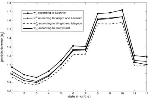
=T ₍₃₂₎

Annual mean values of the precipitable water wp according to the previous

four methods are plotted in Figure 2. We notice that wp obtained with the 4

years of data have the same temporal trend. All methods show a minimum in May and a maximum between July and October. Maximum values are obtained with Leckner model (wL) and the minimum with Magnus using Wright’s

for-mula ( w M

w ). Gueymards method (wG) and Leckner using Wright’s formula (wLw)

give approximately the same mean values (see Table 1). We will use precipitable water values of each method to estimate the Angström turbidity coefficient with the four broadband models. We notice however, that this parameter obtained from the four methods has not a significant effect on turbidity values for a given broadband model. The difference is about 0.1%.

3.3. The Wavelength Exponent

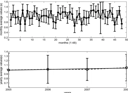
The wavelength exponent α in Equation (1) is related to size distribution of particles. Low values of α _{correspond to large particles and vice versa.}

1.3 0.5

α= ± is suggested by many authors for most natural atmospheres [16]. In our case, we will use MODIS satellite data to obtain the values of this para-meter since we did not dispose of photometric ground measurements. The vari-ation of its monthly mean values over Ghardaïa city is shown in the upper side of Figure 3. Its yearly mean value is plotted in the lower side of Figure 3 where a slightly increase is observed. The annual mean values are 1.0 0.3± _{, 1.0 0.3}± _, 1.0 0.3± _{, 1.1 0.3}± _{for 2005, 2006, 2007 and 2008 respectively. The mean value} of α over the four years is 1.0 0.3± _{and it is in agreement with values} sug-gested by many authors.

3.4. The Ground Albedo

We also used MODIS data to estimate the ground albedo

ρ

g at Ghardaïa city.

(10)

DOI: 10.4236/acs.2019.91008 122 Atmospheric and Climate Sciences Figure 2. Precipitable water according to the four methods.

Table 1. Monthly average values of the total precipitable water using four methods.

L w w M w w L w w G January 1.071 ± 0.038 0.959 ± 0.034 0.990 ± 0.048 1.024 ± 0.037 February 0.985 ± 0.020 0.890 ± 0.019 0.918 ± 0.025 0.941 ± 0.019 March 0.954 ± 0.050 0.870 ± 0.043 0.898 ± 0.061 0.910 ± 0.047 April 1.025 ± 0.064 0.940 ± 0.059 0.970 ± 0.045 0.979 ± 0.061 May 1.147 ± 0.050 1.057 ± 0.045 1.101 ± 0.046 1.098 ± 0.048 June 1.312 ± 0.099 1.215 ± 0.091 1.270 ± 0.102 1.258 ± 0.096 July 1.304 ± 0.019 1.217 ± 0.019 1.272 ± 0.021 1.254 ± 0.019 August 1.676 ± 0.119 1.562 ± 0.053 1.616 ± 0.060 1.610 ± 0.057 September 1.687 ± 0.111 1.560 ± 0.104 1.627 ± 0.116 1.618 ± 0.107 October 1.718 ± 0.114 1.577 ± 0.145 1.642 ± 0.147 1.642 ± 0.137 November 1.202 ± 0.038 1.084 ± 0.036 1.126 ± 0.048 1.147 ± 0.035 December 1.187 ± 0.608 1.087 ± 0.617 1.100 ± 0.622 1.136 ± 0.587 Mean 1.272 ± 0.113 1.168 ± 0.110 1.211 ± 0.117 1.218 ± 0.108

annual mean values plotted in the lower side. The annual mean values are 0.17 0.06± _{, 0.18 0.05}± _{, 0.17 0.05}± _{, 0.18 0.05}± _{for 2005, 2006, 2007 and} 2008 respectively. The

ρ

g mean value over the four years is 0.17 0.05± . We

note also a slightly increase of

ρ

g between 2005 and 2008 with a litte drop in

2007.

3.5. Single Scattering Albedo and Forward Scattering

The value of 0.8 for the single scattering albedo w0 is usually chosen for

(11)

DOI: 10.4236/acs.2019.91008 123 Atmospheric and Climate Sciences Figure 3. Upper-side: Variations of monthly mean values of the wavelength exponent for the period 2005-2008. Lower-side: Variations of yearly mean values of wavelength expo-nent from 2005 to 2008.

Figure 4. Upper-side: Variations of monthly mean values of the ground albedo for the period 2005-2008. Lower-side: Variations of yearly mean values of ground albedo from 2005 to 2008.

suggested by [17] for the forward scattering Fc. We preferred here to use

mod-eling techniques to find these parameters and their temporal variations rather than a constant value. In a recent study, [36] assessed the intrinsic performance of 18 broadband radiative models using high-quality data sets from five sites in widely different climates. All these models are able to predict direct, diffuse and

(12)

global irradiance under clear skies from atmospheric data. Intrinsic perfor-mances of these models were evaluated by comparison between their predictions and high frequency measurements (1-minute time step in four sites, 3-minute in one site). From the 18 models is the Iqbal C [17] model that requires a rela-tively large number of atmospheric inputs and showed consistently high scores of statistical indicators. This model will be considered in our present study to es-timate the required parameters since it offers a better accuracy than the others more conventional models [36]. In addition, the model inputs are those that we need, namely the Angstrom coefficient β , the average surface albedo

ρ

g, the wavelength Angstrom exponent α , the forward scatterance Fc and the aero-sol single scattering albedo w0. Only the last two parameters and the Angstrom

coefficient β_{will be considered since the others are obtained from MODIS}

data (see Sections 3.3 and 3.4). Before proceeding the estimation of the parame-ters, we recall hereafter the main equations of this model described in detail in

[17].

The direct normal irradiance In (W/m2) is given by:

(

)

0 0

0.9751 ,

n sc g w r a

I = I E

τ τ τ τ τ α β

(33) where τ0,

τ

g, τw, τr and

τ α β

a

(

,

)

are respectively the ozone, gas, water,

Rayleigh and aerosol scattering transmittances. Isc and E0 are respectively

the solar constant and the eccentricity correction factor.

The aerosol scattering transmittance, which depends on the Angstrom coeffi-cient β_{and wavelength Angstrom exponent}α, is given by Equation (10).

The global solar irradiance (It) measured with our instruments is the

contri-bution of 2 solar irradiance components given by:

t nh d

I =I +I ₍₃₄₎

where (Inh) is the normal solar irradiance on an horizontal surface and (Id) the

horizontal diffuse solar irradiance. The normal solar irradiance Inh (W/m2) is

given by:

( )

sin nh n

I =I h (35) where h is the elevation angle of Sun in degrees.

The horizontal diffuse solar irradiance Id (W/m2) is a combination of three

individual components, which are the Rayleigh component, Idr (W/m2), the

aerosols scattering component, Ida (W/m2) after the first pass through the

at-mosphere, and the multiple reflection processes between the ground and sky component, Idm (W/m2):

d dr da dm

I =I +I +I ₍₃₆₎

The Idr component which depends on aerosol single scattering albedo w0,

is given by:

( )

(

)

0

( )

0 0 1.02 sin 0.395 1 1 sc dr g w r aa a a I E h I w m m τ τ τ τ τ = − − + (37) where

(

)

(

1.06

)

(

)

0 1 1 1 1 aa w m ma a a

(13)

transmittance due to aerosol absorptance.

The Ida component is related to the forward scatterance Fc:

( )

(

)

0

( )

0 1.02 sin 0.79 1 1 sc da c g w aa c as a a I E h I F F m m τ τ τ τ τ = − − + (38)

The Idm component related to the ground albedo

ρ

g, is given by:

( )

(

)

₁ g a dm g nh dr da g a I ρ I I I ρ ρ ρ ρ = + + − (39) where ρa is the albedo of the cloudless sky, which can be computed with:

(

)

0.0685 1 1 a a c aa F

τ

ρ

τ

  = + − _ − _   (40)

The

(

1−Fc

)

term corresponds to the back-scatterance. The second term on

the right hand side of Equation (40) represents the albedo of cloudless skies due to the presence of aerosols, whereas the first term is the albedo of clean air.

The global solar irradiance (It) on a horizontal surface is then expressed by:

( )

(

sin

)

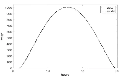
1 1 t nh d n dr da g a I I I I h I I ρ ρ = + = + + − (41)

We will fit the recorded global solar irradiance (Itr) of clear days with Iqbal C

model given by Equation (41). The method consists to solve a nonlinear fitting problem in the least-squares sense i.e. we look for the x-vector coefficients (β, ,w F0 c) that minimize the following residual function:

( )

2

(

( )

)

2

qbal tr qbal i tr

i

I x −I =

∑

I x −I ₍₄₂₎

where Iqbal

( )

x =It

(

β

, ,w F0 c

)

is the Iqbal C model. Figure 5 plots a recorded

global solar irradiance component of a clear day superposed to its fit by Iqbal C model.

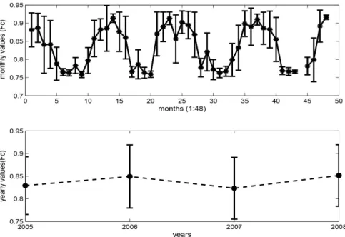
We will apply this process to all global solar irradiance of clear days of the recorded data. The clear days are determined using the novel method developed by [37]. Each fit will give us a value of the aerosol single scattering albedo w0

and a value of the forward scatterance Fc. The monthly and the yearly mean

values of these two parameters are shown in Figure 6 and Figure 7 respectively. The annual mean values vary between 0.80 0.04± and 0.81 0.04± for the aerosol single scattering albedo w0 and between 0.82 0.04± and 0.85 0.04±

for the forward scatterance Fc. We note that the two parameters vary in

oppo-site of phase with each other with particular values during 2007.

4. Results and Discussion

All useful parameters described in the previous section are used to calculate the Angstrom coefficient obtained with the four turbidity models. The coefficients

Dog

β

, βLouch, βPinz and

β

Gyem are respectively calculated with models of

(14)

DOI: 10.4236/acs.2019.91008 126 Atmospheric and Climate Sciences Figure 5. A recorded solar irradiance component of a clear day (full line) superposed to its fit obtained with Iqbal C model (dashed line).

Figure 6. Upper-side: Variations of monthly mean values of the aerosol single scattering albedo w0 for the period 2004-2008. Lower-side: Variations of yearly mean values of the aerosol single scattering albedo w0 from 2005 to 2008.

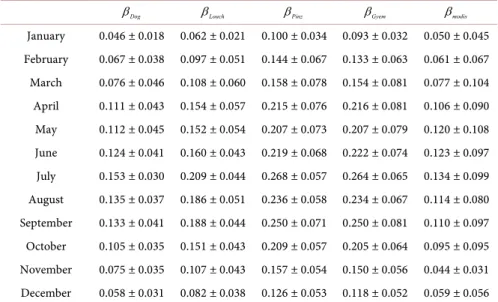
obtained from space data recorded with the MODIS instrument aboard the Ter-ra satellite (NASA). All these Angström turbidity coefficients are shown in Fig-ure 8. Temporal variations of the monthly values of β _{for the period}

2005-2008 are plotted in the upper side of Figure 8. The mean values for each month calculated over the same period are shown in the lower side of this figure. These values are reported in Table 2. We notice from Figure 8 that

β

Gyem and

Pinz

β _{are very close as}

β

_Dog_and β_modis_. β_Louch_{are in the average of all}

(15)

DOI: 10.4236/acs.2019.91008 127 Atmospheric and Climate Sciences Figure 7. Upper-side: Variations of monthly mean values of the forward scatterance Fc for the period 2004-2008. Lower-side: Variations of yearly mean values of the forward scatterance Fc from 2005 to 2008.

Figure 8. Monthly mean values of the angstrom coefficient βDog, βLouch, βPinz, βGyem

and βmodis for the period 2005-2008.

to 100%. We also note that Angström coefficient curves have all the same shape during the period 2005-2008 and along the year where maximum and minimum are respectively during summer and winter months. We can explain it by winds of the south sectors (Sirocco) that characterize the region of Ghardaïa. This kind of winds brings particles of dust and sand with them, which increases the Angström coefficient. It is well observed in Figure 6 where w0 is higher in

summer and consequently contributes to light extinction due to aerosol scatter-ing. The period of winter is characterized by rains (see Figure 2) that wash the atmosphere and diminish turbidity variables.

Annual mean values of β_{obtained from the models and from space are}

plotted in Figure 9 and given in Table 3. We can notice three points: 1)

β

Pinz 

β

Gyem>

β

Louch >

β

modis 

β

Dog

(16)

DOI: 10.4236/acs.2019.91008 128 Atmospheric and Climate Sciences Table 2. Monthly average values of the Angström turbidity coefficient according to the fifth methods.

Dog

β βLouch βPinz βGyem βmodis

January 0.046 ± 0.018 0.062 ± 0.021 0.100 ± 0.034 0.093 ± 0.032 0.050 ± 0.045 February 0.067 ± 0.038 0.097 ± 0.051 0.144 ± 0.067 0.133 ± 0.063 0.061 ± 0.067 March 0.076 ± 0.046 0.108 ± 0.060 0.158 ± 0.078 0.154 ± 0.081 0.077 ± 0.104 April 0.111 ± 0.043 0.154 ± 0.057 0.215 ± 0.076 0.216 ± 0.081 0.106 ± 0.090 May 0.112 ± 0.045 0.152 ± 0.054 0.207 ± 0.073 0.207 ± 0.079 0.120 ± 0.108 June 0.124 ± 0.041 0.160 ± 0.043 0.219 ± 0.068 0.222 ± 0.074 0.123 ± 0.097 July 0.153 ± 0.030 0.209 ± 0.044 0.268 ± 0.057 0.264 ± 0.065 0.134 ± 0.099 August 0.135 ± 0.037 0.186 ± 0.051 0.236 ± 0.058 0.234 ± 0.067 0.114 ± 0.080 September 0.133 ± 0.041 0.188 ± 0.044 0.250 ± 0.071 0.250 ± 0.081 0.110 ± 0.097 October 0.105 ± 0.035 0.151 ± 0.043 0.209 ± 0.057 0.205 ± 0.064 0.095 ± 0.095 November 0.075 ± 0.035 0.107 ± 0.043 0.157 ± 0.054 0.150 ± 0.056 0.044 ± 0.031 December 0.058 ± 0.031 0.082 ± 0.038 0.126 ± 0.053 0.118 ± 0.052 0.059 ± 0.056

Table 3. Annual mean values of the Angström turbidity coefficient obtained with the four methods and from space.

Dog

β βLouch βPinz βGyem βmodis

2005 0.090 ± 0.035 0.128 ± 0.045 0.176 ± 0.058 0.171 ± 0.060 0.093 ± 0.081 2006 0.095 ± 0.037 0.135 ± 0.048 0.190 ± 0.065 0.185 ± 0.070 0.090 ± 0.063 2007 0.106 ± 0.040 0.142 ± 0.049 0.193 ± 0.065 0.195 ± 0.071 0.104 ± 0.076 2008 0.104 ± 0.034 0.146 ± 0.046 0.201 ± 0.060 0.194 ± 0.064 0.106 ± 0.083

Figure 9. Annual mean values of the angstrom coefficient βDog, βLouch, βPinz, βGyem

and βmodis for the period 2005-2008.

2) βPinz,

β

Gyem, βLouch, βmodis and

β

Dog increases from 2005 to 2008

3)

β

Gyem, βmodis,

β

Dog and βPinz shows a slight increase in 2007 contrary

to βLouch

The first point was also reported by [38] when they analyzed the atmospheric turbidity levels at Taichung Harbor near Taiwan Strait. This was observed too by

(17)

DOI: 10.4236/acs.2019.91008 129 Atmospheric and Climate Sciences [24] when they studied the atmospheric turbidity for Hong Konghowed and showed that βPinz >βLouch.

The second point is related to the city environment. The recent study of [39]

showed that the urban aerosols during the same period of study predominate the other types of aerosols. It is explained by the presence of many companies of crusher plants and industrial companies installed around the city and agglome-ration that increased from year to year.

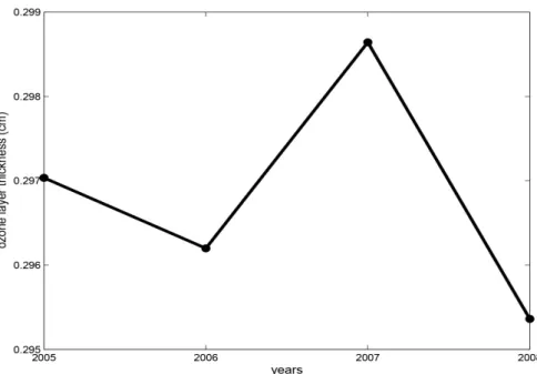
The third point is probably related to the ozone layer thickness that presents a slight increased in 2007 as shown in Figure 10. Indeed, the ozone layer thickness decreased steadily from 2005 to 2008 but increased in 2007.

β

Gyem, βmodis,

Dog

β

and βPinz seem to be more sensitive to ozone layer thickness than βLouch.

Recurrent values of Angström turbidity coefficient and its cumulative fre-quency distribution were also analyzed during the period 2005-2008. The tur-bidity coefficient occurrence provides useful information about the site and its turbidity conditions. The cumulative frequency distribution is adapted to inform on the percentage of clear days where turbidity exceeds a given limit. Figure 11

plots the frequency distribution of

β

Dog, βLouch, βPinz,

β

Gyem and βmodis. We

observe that the distribution is not Gaussian but looks like a Poisson law. We notice that the maximum recurrent value of:

1)

β

Dog is 0.03 with a frequency of about 10.5%

2) βLouch is 0.07 with a frequency of about 8.3%

3) βPinz is 0.10 with a frequency of about 6.3%

4)

β

Gyem is 0.09 with a frequency of 7.4%

5) βmodis is 0.02 with a frequency of about 9.9%

The cumulative frequency distribution of Angström turbidity coefficient for each model is calculated and plotted in Figure 12. The various degrees of at-mospheric clearness deduced from each cumulative frequency distribution [32] [38] are given in Table 4. We observe from the Table that

β

Dog and βmodis

yield the same and the maximum “clean to clear” conditions with respect to other methods. The minimum “clean to clear” conditions is yielded by βPinz

model. The maximum values for the “clean to turbid” conditions are yielded by

Pinz

β _and

β

_Gyem_{and the minimum by}β_modis_.

β

_Dog_{yields the lowest values}

for “turbid to very turbid” conditions and both

β

Gyem and βPinz models give

the highest.

This analysis based on the cumulative frequency distribution confirms as be-fore that Louche?s model gives a middle value of sky conditions in comparison with the other models. We will then consider its values as those for Ghardaïa and we may conclude that major sky conditions under cloudless days are be-tween clean and turbid for this region.

5. Conclusions

The Angström turbidity coefficient β_{is calculated with four broadband}

(18)

DOI: 10.4236/acs.2019.91008 130 Atmospheric and Climate Sciences Figure 10. Annual average values of the ozone layer thickness for the period 2004-2008.

Figure 11. Frequency of occurrences for angstrom coefficient (βPinz, βGyem, βLouch, modis

β , βDog, and βmodel) measured between 2005 and 2008.

Figure 12. Cumulative frequency distribution for angstrom coefficient values (βPinz, Gyem

(19)

DOI: 10.4236/acs.2019.91008 131 Atmospheric and Climate Sciences Table 4. Various degrees of atmospheric clearness.

0.1 β≤ (clean to clear) 0.1< ≤β 0.2 (clear to turbid) 0.2 β>

(turbid to very turbid)

Pinz β _26% _46% _28% Gyem β 31% 44% 25% Louch β _51% _38% _11% Dog β 69% 30% 1% modis β 69% 23% 8%

2005-2008 at Ghardaïa in the south of Algeria. Data recorded with MODIS aboard Terra satellite (NASA) were also used. These models are referred to Dogniaux (

β

Dog), Louche (βLouch), Pinazo (βPinz), Gueymard (

β

Gyem) and to

MODIS βmodis. Results obtained from model calculations showed that

β

Gyem

and βPinz are very close as the couple

β

Dog and βmodis while βLouch have

middle values in regard to the other models. The differences between β values are large and range from 50% to 100% between models.

All models and space data showed that the temporal variations of the Angström turbidity coefficients during 2005-2008 have the same trend. An in-crease of the annual mean values of β was observed during this period, which is explained by the city environment and aerosols types. In addition, a slight in-crease of β was observed in 2007 except for βLouch. This jump was attributed

to the ozone layer thickness leading to affirm that these models are sensitive to this atmospheric component.

We finally completed the comparison of the models by analyzing the occur-rence and cumulative frequency distribution of the Angström turbidity coeffi-cients. Results showed for all models that the frequency distribution is not Gaus-sian but looks like a Poisson law. The maximum recurrent values for

β

Dog is

found near 0.03, near 0.07 for βLouch, near 0.10 for βPinz, near 0.09 for

β

Gyem

and near 0.02 for βmodis. The cumulative frequency distribution study revealed

also that

β

Dog and βmodis yield the maximum “clean to clear conditions” with

respect to the other models while βPinz and

β

Gyem have the minimum. The

opposite was observed on the same pairs of β _{with regard to the “clear to}

tur-bid” and “turbid to very turtur-bid” conditions. The Louche model gave middle val-ues of sky conditions compared to the other models. This result leads us to con-sider Louche’s model values for Ghardaïa city. The major sky conditions under cloudless days for this semi arid region are then between clean and turbid.

Conflicts of Interest

The authors declare no conflicts of interest regarding the publication of this pa-per.

References

(20)

City. Atmospheric Research, 450, 46-51.

https://doi.org/10.1016/j.atmosres.2013.03.009

[2] Lopez, G. and Batlles, F.J. (2004) Estimate of the Atmospheric Turbidity from Three Broad-Band Solar Radiation Algorithms, a Comparative Study. Annales Geophysi-cae, 22, 2657-2668. https://doi.org/10.5194/angeo-22-2657-2004

[3] Angström, A. (1929) On the Atmospheric Transmission of Solar Radiation and on Dust in the Air. Geografiska Annaler, 2, 156-166. https://doi.org/10.2307/519399

[4] Angström, A. (1930) On the Atmospheric Transmission of Solar Radiation. Geogra-fiska Annaler, 12, 130-159. https://doi.org/10.2307/519561

[5] Angström, A. (1961) Techniques of Determining the Turbidity of the Atmosphere.

Tellus, 13, 214-223. https://doi.org/10.3402/tellusa.v13i2.9493

[6] Angström, A. (1964) The Parameters of Atmospheric Turbidity. Tellus, 16, 64-75.

https://doi.org/10.3402/tellusa.v16i1.8885

[7] Dogniaux, R. (1974) Repréntations analytiques des composantes du rayonnement lumineux solaire. Conditions du ciel serein. Institut Royal de Métiorologie de Bel-gique, Serie A No. 83, 3-24.

[8] Louche, A., Peri, G. and Iqbal, M. (1986) An Analysis of Linke Turbidity Factor.

Solar Energy, 37, 393-396. https://doi.org/10.1016/0038-092X(86)90028-9

[9] Pinazo, J.M., Canada, J. and Boscá, J.V. (1995) A New Method to Determine the Angström’s Turbidity Coefficient: Its Application to Valencia. Solar Energy, 54, 219-226. https://doi.org/10.1016/0038-092X(94)00117-V

[10] Gueymard, C. and Vignola, F. (1998) Determination of Atmospheric Turbidity from the Diffuse-Beam Broadband Irradiance Ratio. Solar Energy, 63, 135-146.

https://doi.org/10.1016/S0038-092X(98)00065-6

[11] Grenier, J. C., De La Casiniere, A. and Cabot, T. (1994) A Spectral Model of Linke’s Turbidity Factor and Its Experimental Implications. Solar Energy, 52, 303-314.

https://doi.org/10.1016/0038-092X(94)90137-6

[12] Kasten, F. (1980) A Simple Parameterization of the Pyrheliometric Formula for De-termining the Linke Turbidity Factor. Meteorologische Rundschau, 33, 124-127. [13] Kasten, F. (1996) The Linke Turbidity Factor Based on Improved Values of the

Integral Ayleigh Optical Thickness. Solar Energy, 56, 239-244.

https://doi.org/10.1016/0038-092X(95)00114-7

[14] Kasten, F. (1988) Elimination of the Virtual Diurnal Variation of the Linke Turbid-ity Factor. Meteor. Rdsch, 41, 93-94.

[15] Trabelsi, A. and Masmoudi, M. (2011) An Investigation of Atmospheric Turbidity over Kerkennah Island in Tunisia. Atmospheric Research, 101, 22-30.

[16] Canada, J., Pinazo, J.M. and Boscá, J.V. (1993) Determination of Angström’s Tur-bidity Coefficient at Valencia. Renewable Energy, 3, 621-626.

https://doi.org/10.1016/0960-1481(93)90068-R

[17] Iqbal, M. (1983) An Introduction to Solar Radiation. Academic Press, Toronto. [18] Machler, M.A. (1983) Parameterization of Solar Radiation under Clear Skies. M.Sc.

Thesis, University of British Columbia, Vancouver.

[19] Machler, M.A. and Iqbal, M. (1985) A Modification of the ASHRAE Clear Sky Ir-radiation Model. ASHRAE Transactions, 91, 106-115.

[20] Louche, A., Maurel, M., Simonet, O., Peri, G. and Iqbal, M. (1987) Determination of Angström’s Turbidity Coefficient from Direct Solar Irradiance Measurements. Solar

(21)

Energy, 38, 89-96.https://doi.org/10.1016/0038-092X(87)90031-4

[21] Gueymard, C. (1995) SMARTS2, Simple Model of the Atmospheric Radiative Transfer of Sunshine: Algorithms and Performance Assessment. Rep. FSEC-PF-270-95, Florida Solar Energy Center.https://doi.org/10.1016/j.atmosres.2007.08.003

[22] Chaabane, M. (2008) Analysis of the Atmospheric Turbidity Levels at Two Tunisian Sites. Atmospheric Research, 87, 136-146.

[23] Chaiwiwatworakul, P. and Chirarattananon, S. (2004) An Investigation of Atmos-pheric Turbidity of Thai Sky. Energy and Buildings, 36, 650-659.

https://doi.org/10.1016/j.enbuild.2004.01.032

[24] Li, D.H.W. and Lam, J.C. (2002) A Study of Atmosphere Turbidity for Hong Kong.

Renewable Energy, 25, 1-13.https://doi.org/10.1016/S0960-1481(01)00008-8

[25] Janjai, S., Kumharn, W. and Laksanaboonsong, J. (2003) Determination of Angstrom’s Turbidity Coefficient over Thailand. Renewable Energy, 28, 1685-1700.

https://doi.org/10.1016/S0960-1481(03)00010-7

[26] Karayel, M., Navvab, M., Ne’eman, E. and Selkowitz, S. (1984) Zenith Luminance and Sky Luminance Distributions for Daylighting Calculations. Energy and Build-ings, 6, 283-291.https://doi.org/10.1016/0378-7788(84)90060-4

[27] Littlefair, P.J. (1994) The Luminance Distributions of Clear and Quasi-Clear Skies.

Proceedings of the CIBSE National Lighting Conference, Cambridge, 267-283. [28] Perez, R., Seals, R. and Michalsky, J. (1993) All-Weather Model for Sky Luminance

Distribution-Preliminary Configuration and Validation. Solar Energy, 50, 235-245.

https://doi.org/10.1016/0038-092X(93)90017-I

[29] Ichoku, C., Kaufman, Y.J., Remer, L.A. and Levy, R. (2004) Global Aerosol Remote Sensing from MODIS. Advances in Space Research, 34, 820-827.

https://doi.org/10.1016/j.asr.2003.07.071

[30] Torres, O., Decae, R., Veefkind, P. and de Leeuw, G. (2002) OMI Aerosol Retrieval Algorithm. Algorithm Theoretical Baseline Document: Clouds, Aerosols, and Sur-face UV Irradiance. Vol. III, ATBD-OMI-03, Version 2.0.

[31] Wright, J., Perez, R. and Michalsky, J. (1989) Luminous Efficacy of Direct Irra-diance: Variations with Insolation and Moisture Conditions. Solar Energy, 42, 387-394.

[32] Leckner, B. (1978) The Spectral Distribution of Solar Radiation at the Earth’s Sur-face. Solar Energy, 20, 143-150.https://doi.org/10.1016/0038-092X(78)90187-1

[33] Gueymard, C. (1994) Analysis of Monthly Average Atmospheric Precipitable Water and Turbidity in Canada and Northern United States. Solar Energy, 53, 57-71.

https://doi.org/10.1016/S0038-092X(94)90606-8

[34] Boscaa, J.V., Canada, J., Pinazo, J.M. and Ruiz, V. (1996) Angström’s Turbidity Coefficient in Seville, Spain in the Years 1990 and 1991. International Journal of Ambiant Energy, 17, 171-178.https://doi.org/10.1080/01430750.1996.9675240

[35] Gueymard, C. (1989) A Two-Band Model for the Calculation of Clear Sky Solar Ir-radiance, Illuminance, and Photosynthetically Active Radiation at Earth’s Surface.

Solar Energy, 43, 253-265.https://doi.org/10.1016/0038-092X(89)90113-8

[36] Gueymard, C. (2012) Clear-Sky Irradiance Predictions for Solar Resource Mapping and Large-Scale Applications: Improved Validation Methodology and Detailed Performance Analysis of 18 Broadband Radiative Models. Solar Energy, 86, 2145- 2169.

[37] Djafer, D., Irbah, A. and Zaiani, M. (2017) Identification of Clear Days from Solar Irradiance Observations Using a New Method Based on the Wavelet Transform.

(22)

Renewable Energy, 101, 347-355.https://doi.org/10.1016/j.renene.2016.08.038

[38] Wen, C.C. and Yeh, H.H. (2009) Analysis of Atmospheric Turbidity Levels at Tai-chung Harbor near the Taiwan. Atmospheric Research, 94, 168-177.

[39] Zaiani, M., Djafer, D. and Chouireb, F. (2016) Classification of Aerosol Types over Ghardaia, Algeria, Based on MODIS Data. International Journal of Environmental Science and Development, 7, 745-749.