Design of a very high frequency resonant boost DC-DC converter

Design of a Very High Frequency Resonant Boost

DC-DC Converter

by

Justin Burkhart

B.S., University of Massachusetts (2006)

Submitted to the Department of Electrical Engineering and Computer Science in partial fulfillment of the requirements for the degree of

Master of Science

at the

MASSACHUSETTS INSTITUTE OF TECHNOLOGY

June 2010

@

Departm t of Electrical Engineering and Computer Science May 21, 2010

A

1- ' /

/,

Associate Professor of Electrical Engineering Thesis Supervisor A7 j-Accepted by MA5SACHUSETTS INSTITUTE, OF TECHNOLOGY

JUL 12 2010

LIBRARIES

Design of a Very High Frequency Resonant Boost DC-DC Converter by

Justin Burkhart

Submitted to the Department of Electrical Engineering and Computer Science on May 21, 2010, in partial fulfillment of the

requirements for the degree of Master of Science

Abstract

T

resonant boost converter. The topology examined features low parts count and fast transient response but suffers from higher device stresses compared to other topologies that use a larger number of passive components.

A new design methodology for the proposed converter topology is developed. This design procedure - unlike previous design methodologies for similar topologies - is based on direct analysis of the topology and does not rely on lengthy time-domain simulation sweeps across circuit parameters to identify good designs.

Additionally, a method to design semiconductor devices that are suitable for use in the pro-posed VHF power converter is presented. When the main semiconductor switch is fabricated in a integrated power process where the designer has control over the device layout, large performance gains can be achieved by considering parasitics and loss mechanisms that are important to operation at VHF when designing the device. A method to find the optimal device for a particular converter design is presented.

The new design methodology is combined with the device optimization technique to enable the designer to rapidly find the optimal combination of converter and device design for a given specification.

To validate the proposed converter topology, design methodology, and device optimization, a 75 MHz prototype converter is designed and experimentally demonstrated. The perfor-mance of the prototype closely matches that predicted by the design procedure, and achieves good efficiency over a wide input voltage range.

Acknowledgements

I would like to thank my advisor Professor Dave Perreault for sharing his extensive knowl-edge with me over the past two years. I am thankful for the guidance and support that he has given me throughout this project. I have learned far more than I expected to when I first began here, and that is largely due to him.

To all of my friends in Dave's group, its been a pleasure spending the past two year here with all of you. Its hard to believe how fast the time has gone by.

Tony Sagneri has been a continuous source of help to me throughout this whole project. His willingness to drop what he was doing to help me whenever I was stuck on a problem has been of tremendous value to me.

My thanks goes to Irwin and Joan Jacobs for their generosity in supporting my education, and to Texas Instruments for supporting my research. Specifically I'd like to thank Roman Korsunsky for all of his support through out the course of this project, and especially for the help getting my chip fabricated.

I'd like to express my thanks and gratitude to my Parents. You've been a constant source of encouragement throughout my whole life, and I'm sure that I wouldn't be here today without your love and support.

Most importantly, I'd like to thank my wife Jennifer for always being there for me. Your support throughout our time here means a lot to me. I couldn't of made through without you by my side. I love you.

Contents

1 Introduction 17

1.1 Thesis Contribution and Organization . . . . 20

2 VHF Converter Architecture 23 2.1 The Class-E Inverter . . . . 23

2.1.1 Design Procedure . . . . 24

2.1.2 Drawbacks of the Class-E Inverter . . . . 28

2.2 Class-E DC/DC converter . . . . 30

2.2.1 Problems with Hard-Switched Rectifiers . . . . 31

2.2.2 Resonant Rectifiers . . . . 31

2.2.3 DC-DC Converter Topology . . . . 35

2.2.4 Converter Control . . . . 36

2.2.5 Resonant Input Inductor . . . . 38

2.2.6 Mitigation of Frequency Dependent Loss Mechanisms . . . . 39

2.3 Relation to Other Converters . . . . 40

3 Design Methodology 43 3.1 Inverter Analysis . . . . 45

3.2 Rectifier Analysis . . . . 55

4 Semiconductor Devices 65 4.1 Device Model and Loss Mechanisms . . . . 65

4.2 Device Layout Optimization . . . . 67

4.2.1 Layout of a LDMOS Transistor . . . . 68

Contents

4.2.3 Semiconductor Optimization . . . . 4.2.4 Design of an Interconnect Network . . . .

5 Converter Design

5.1 Device Modeling . . . .

5.1.1 MOSFET Model . . . .

5.1.2 Parasitic Capacitances . . . .

5.1.3 On Resistance . . . . 5.1.4 Compensation for Non-Linear 5.2 Design Example . . . . 5.2.1 Select ws . . . . 5.2.2 Select #1 . . . . 5.2.3 Select w . . . . .. 5.2.4 Simulation Results . . . . 5.3 Experimental Results. . . . . Device 6 Conclusion A SPICE Code A .1 Chapter 2 . . . . A.1.1 SPICE Code to Generate Figure 2.2 A.1.2 SPICE Code to Generate Figure 2.7 A.1.3 SPICE Code to Generate Figure 2.8 A.1.4 SPICE Code to Generate Figure 2.11 A.1.5 SPICE Code to Generate Figure 2.14 A.1.6 SPICE Code to Generate Figure 2.17 A.1.7 SPICE Code to Generate Figure 2.21 A .2 Chapter 5 . . . .

A.2.1 SPICE Code to Generate Figure 5.19 A.2.2 SPICE Code to Generate Figure 5.20

-8-Capacitance 101 103 103 103 104 105 106 107 108 109 110 110 111

Contents

B Design Methodology MATLAB Scripts 121

B.1 MATLAB Code to Generate Figures 3.4 and 3.7 .... ... 121

C Device Layout Optimization MATLAB Scripts 131

C.1 MATLAB Code to Generate Figures 4.3 -4.6 ... 131

C.2 MATLAB Code to Generate Figures 4.11 and 4.12 ... 137

C.3 MATLAB Code to Generate Figure 4.15 ... 141

D Design Example MATLAB Scripts 145

D.1 MATLAB Script to generate Figure 5.10 ... ... 145 D.2 MATLAB Script to generate Figures 5.11, 5.12, and 5.13 ... 149 D.3 MATLAB Script to generate Figures 5.15, 5.16, and 5.17 ... 153

E Experimental Prototype Design 159

List of Figures

1.1 Schematic of a linear regulator circuit. . . . . 17

1.2 Schematic of a buck converter . . . . 18

1.3 Buck converter waveforms . . . . 18

1.4 Notional switch waveforms during commutation . . . . 20

2.1 Schematic of the Class-E Inverter . . . . 24

2.2 Simulated waveforms from a SPICE simulation of an ideal class-e Inverter operating with a switching frequency of 100 MHz and an input voltage of 12 Volts. Component values are: LF = 10uH, CE = 67.7pF, CR = 105pF, LR = 34.1nH, and RLOAD=5 Ohms. Simulation script is included in Appendix A. 25 2.3 Diagram showing the switching times of the class-e inverter . . . . 25

2.4 Schematic of a class-e inverter with ideal components used for analysis. . . 26

2.5 Plot showing the relation between the quality factor and resonant frequency of the load leg of a class-e inverter . . . . 28

2.6 Class-e inverter component values plotted versus the resonant frequency of the load leg of the inverter . . . . 29

2.7 Simulated class-e inverter waveforms using component values resulting from the design procedure. The inverter is designed for a switching frequency of 100 MHz and an input voltage of 5 Volts. Simulation script is included in A ppendix A . . . . . 29

2.8 Simulated waveforms of a class-e inverter showing how VD(t) varies with an increased load resistance. Component values are: LF = 10uH, CE = 67.7pF, CR = 105pF, LR = 34.1nH, and RLOAD is varied from 5 to 10 Ohms. Simulation script is included in Appendix A. . . . . 30

2.9 Block diagram of a resonant DC/DC converter . . . . 31

2.10 Hard-switched rectifier circuits.. . . . . . . . 32

2.11 Simulated waveforms of the hard-switched rectifier circuits of Figure 2.10 showing the effect that including parasitics has on operation at VHF. Sim-ulation performed with VAC = 10 Volts, IDC = 1 Amp, LPAR = 3 nH, and CPAR = 30 pF. Simulation script is included in Appendix A. . . . . 32

-List of Figures

2.12 Schematic of a series loaded resonant rectifier circuit. Note that the AC voltage source must pass the dc load current. . . . . 33 2.13 Schematic of a series loaded resonant rectifier circuit with extra capacitance

for converter tuning and dominant parasitic components included . . . . 34 2.14 Simulated waveforms from the resonant rectifier of Figure 2.13 both with and

without parasitics included. Simulation script is included in Appendix A. . 34 2.15 Schematic of a resonant boost DC/DC converter made by joining together a

class-e inverter and a series loaded resonant rectifier. . . . . 35 2.16 Simulated waveforms from the boost converter of Figure 2.15 operating at

100 MHz with an input voltage of 12 Volts and an output voltage of 30 Volts. 36 2.17 Simulated converter waveforms showing the effect of decreasing the load

re-sistance by a factor of two. Simulation script is included in Appendix A. . . 37 2.18 Block diagram of the boost converter control system . . . . 37 2.19 Simulated waveforms of the start-up transient from two converter designs,

both designed to operate with an input voltage of 12 Volts, an output voltage of 30 Volts, and a switching frequency of 100 MHz. One design uses LF=3 pH and is labeled "Choke Inductor", and the other design uses LF=40 nH and is labeled "Resonant Inductor" . . . . 38 2.20 Schematic of the converter circuit used to gain a qualitative understanding

of the effects of reducing the size of LF . . - . .. - - . - - - . .. . 39 2.21 Simulated converter waveforms showing the error in equation (2.20) for a 100

MHz converter with an input voltage of 12 Volts, an output Voltage of 30 Volts, and LF=40 pH. Simulation script is included in Appendix A . . . . . 40 3.1 Schematic of the proposed DC-DC converter topology showing parasitic

ca-pacitances that limit the available design space. . . . . 43 3.2 Schematic of the inverter used for analysis. The rectifier is modeled as a

sinusoidal current source labeled IRECT . - .. . . - -. . . . . 45 3.3 Sample illustrative waveforms for the inverter circuit of Figure 3.2. . . . . . 45 3.4 Closed form solution to the inverter. Solution assumes an input and output

voltage of 12 and 30 Volts and an output power of 7 Watts.

#1

sinusoidal voltage source labeled VAC . . . . . - - - -. -. . . . 55 3.6 Sample illustrative waveforms for the rectifier circuit of Figure 3.5. . . . . . 55

List of Figures

3.7 Numerical solution to the rectifier. Solution assumes an input and output voltage of 12 and 30 Volts and an output power of 7 Watts.

#1

(t).

tran-sistor cell. . . . . 68 4.3 Plots showing how the major intrinsic parasitic components of the LDMOS

transistor vary with device and finger size. . . . . 71 4.4 Plot of the gate time-constant for intrinsic parasitics vs device and finger size. 71 4.5 Predicted converter loss vs device and finger size for a converter that boosts

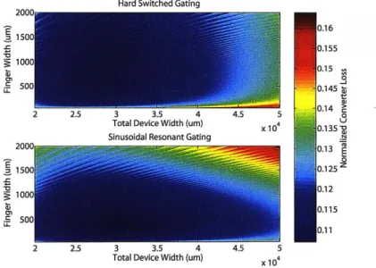
12 Volts to 30 Volts with a switching frequency of 75 MHz, an output power of 15 Watts, an inverter resonant frequency of 63.75 MHz, and the rectifier's current phase set to -1 radian . . . . 72 4.6 Predicted converter loss vs device and finger size for a converter that boosts

12 Volts to 30 Volts with a switching frequency of 75 MHz, an output power of 7 Watts, an inverter resonant frequency of 63.75 MHz, and the rectifier's current phase set to -1 radian .. . . . .I . . . . 72 4.7 Schematic of the proposed DC-DC converter topology showing parasitic

ca-pacitances that limit the available design space. . . . . 73 4.8 Drawings of a LDMOS transistor broken down into 16 fingers and arranged

into various different aspect ratios. . . . . 74 4.9 Drawing showing the scheme used to connect the LDMOS finger gates. . . . 75 4.10 Schematic of the LDMOS gate model for a single finger. . . . . 76 4.11 Plots showing the gate resistance and capacitance vs. the width of the metal

used to connect the gates. ... ... 76 4.12 Plots calculating the loss of a 75 MHz resonant gate driver and gate

time-constant using the parasitic values from Figure 4.11. . . . . 77 4.13 Drawing showing the scheme used to connect the LDMOS drain and source

term inals. . . . . 78 4.14 Schematic of the LDMOS drain-to-source interconnection model for a single

row of fingers. . . . . 78 4.15 Predicted drain-to-source resistance vs. taper angle for two, three, and four

rows of fingers. The device has 100 fingers each with a width of 450 pm. . . 79 4.16 Photograph of the designed LDMOS transistor layout. . . . . 80 5.1 MOSFET model that is preferred for VHF converter design. . . . . 82

-List of Figures

5.2 Schematic of the test setup used to measure the device parasitic capacitances. 82 5.3 Photograph of the PCB used to measure the device capacitances . . . . 83 5.4 Measured Coss data. The model of equation (5.1) is also plotted to show

the good fit. Model parameters are: Cj0=121 pF, V3 = 1.2701 Volts, and M

= 0.4123. . . . . 84 5.5 M easured CIss data. . . . . 84 5.6 Measured reverse biased junction capacitance of S310 Schottky diode

man-ufactured by Fairchild. The model of equation (5.1) is also plotted to show the good fit. Model parameters are: Cj,=267 pF, V3 = 0.365 Volts, and M

= 0.421. . . . . 85

5.7 Schematic of the setup used to measure RDS-ON. . .. . . . . . .. . - . . 86 5.8 M easured RDS-ON data. . . . . 86 5.9 Plots showing equation (5.6) graphically with the fitting parameters for the

LDMOS capacitance Coss and for the diode's junction capacitance. .... 88 5.10 Output from the combined design methodology and device optimization

pro-cedure for a converter with an input voltage of 12 Volts, an output voltage of 30 Volts, and an output power of 7 Watts. The MATLAB script used to generate this figure is included in Appendix D.1 . . . . 89 5.11 Plots generated from the design methodology to show the inverter's passive

component sizes as a function of the rectifier's current phase,

41

component sizes as a function of the rectifier's current phase,

41

optimiza-tion to show the converter's predicted efficiency and the optimal device size (for each design point). Solution is for a converter with an input voltage of 12 Volts, an output voltage of 30 Volts, an output power of 7 Watts, and a switching frequency of 75 MHz. . . . . 91 5.14 Plot showing the slope of VC(t) as a function of the rectifier's current phase,

#1

List of Figures

5.15 Plots generated from the design methodology to show the inverter's passive component sizes as a function of the resonant frequency of the inverter. So-lution is for a converter with an input voltage of 12 Volts, an output voltage of 30 Volts, an output power of 7 Watts, a switching frequency of 75 MHz, and the rectifier's current phase of

#1=-1

component sizes as a function of the resonant frequency of the inverter. So-lution is for a converter with an input voltage of 12 Volts, an output voltage of 30 Volts, an output power of 7 Watts, a switching frequency of 75 MHz,

and the rectifier's current phase of

#1=-1

optimiza-tion to show the converter's predicted efficiency and the optimal device size (for each design point). Solution is for a converter with an input voltage of 12 Volts, an output voltage of 30 Volts, an output power of 7 Watts, a switching

frequency of 75 MHz, and the rectifier's current phase of

#1=-1

5.18 Plot showing the peak energy stored in the inverter in a cycle normalized to the energy delivered to the load in a cycle as a function of the resonant frequency of the inverter for a converter with an input voltage of 12 Volts, an output voltage of 30 Volts, an output power of 7 Watts, and a switching

frequency of 75 MHz, and the rectifier's current phase of

_#1=-1

5.19 Simulation results for a converter with an input voltage of 12 Volts, an output voltage of 30 Volts, an output power of 7 Watts, and a switching frequency of 75 MHz, the rectifier's current phase of

#1=-1

voltage of 30 Volts, an output power of 7 Watts, and a switching frequency of 75 MHz and a duty ratio of 50%, the rectifier's current phase of

#1=-1

midi-spring family from Coilcraft, and the diode is an S310 Schottky diode from Comchip Technology. The MOSFET is a custom LDMOS device fabri-cated from an integrated power process. The converter operates at 75 MHz with a 50% duty cycle. The device characteristics of S1 are shown in Figures 5.4, 5.5, and 5.8... . . . . . . . . . 98

List of Figures

5.23 Measured converter waveforms compared to simulated waveforms in SPICE. 99

5.24 Measured converter waveforms over the input voltage range. . . . . 100

5.25 Measured efficiency (not including gate drive loss) versus input voltage for two specified output power levels. Output power is controlled by on-off mod-ulating the converter with a PWM signal at 1 MHz. . . . . 100

E.1 Experimental schematic of the power stage. . . . . 159

E.2 Experimental schematic of the gate drive circuit. . . . . 159

E.3 PCB top metal layout. . . . . 160

E.4 PCB first inner metal layout. . . . . 161

E.5 PCB second inner metal layout. . . . . 161

E.6 PCB bottom metal layout . . . . 162

List of Tables

1.1 _{Summary of buck converter loss mechanisms . . . . 20} 4.1 _{Overall size of a LDMOS transistor composed of 100 fingers each with a}

width of 450 pm . . . . 74 5.1 Target converter specifications.... . . . . . . . 81 5.2 _{Parameters to fit equation (5.1) to measured the junction capacitance data}

for the S310 diode. . . . . 83 5.3 _{Parameters to fit equation (5.1) to measured the Coss data. . . . . 85} 5.4 Component values as predicted by the design methodology for a converter

with an input voltage of 12 Volts, an output voltage of 30 Volts, an output power of 7 Watts, and a switching frequency of 75 MHz, the rectifier's current phase of

#1=-1

-Chapter 1

Introduction

P

system. In battery operated applications, power converters supply the constant voltage that electronics require as the battery voltage drops from discharge. Systems that need multiple DC supply voltages require the use of a power converter to convert one DC voltage to another.

VIN Control VoUT

Figure 1.1: Schematic of a linear regulator circuit.

A linear regulator shown in Figure 1.1 is a simple way to convert one DC voltage to another, but it has two major problems. First, the output voltage must always be less than the input. Consider a system that is powered by a Lithium-Ion battery. Fully charged, the battery supplies 4.3 Volts, but when discharged it only supplies 3 Volts. Many electronic systems require a supply voltage of 3.3 Volts. Thus, if a linear regulator is used the system cannot be operated throughout the entire discharge cycle. The second major drawback of using a linear regulator is efficiency. Since the load current must pass through the regulation device, the converter consumes a power equal to the load current times the change in voltage. This leads to a best-case efficiency of:

VOUT VIN

When the the conversion ratio is large this efficiency is not acceptable. Thus, there is a need for conversion technology that can efficiently convert from one DC voltage to another, and be able to convert up and down. Both of these needs are met by switching power converters. Figure 1.2 shows the schematic of a buck converter. This converter achieves 100% efficiency with ideal components.

Introduction Ideal Lossless Switch Filter - + VDS -+1 + I" + +

-r-VIN -_ Vx VouT RLOAD _{N + VxRLOAD}

VIN :

~---..

--VNIxVo~

Ideal Converter

_{Real Implimentation}

Figure 1.2: Schematic of a buck converter

VVOUT 3 .1.56 2.5 --1.54 I0i -i -- I 2 . . . .1.52 r -' 4 - I - FC=0.1F .1.5 . -- - - --- F =0.3F . Fc=0.5F 1.44 0 5 10 15 20 25 30 0 10 20 30 Time (ps) Time (ps)

Figure 1.3: Buck converter waveforms

The converter operates by controlling the switch to generate a square wave, shown at V, in Figure 1.3. This square wave is filtered using a lossless LC filter to produce a DC output equal to the average value of the square wave, and the output voltage is controlled by varying the duty cycle of the square wave. The output voltage of the converter contains some ripple components in addition to the desired DC voltage. The ripple is reduced by lowering the cutoff frequency (FC in Figure 1.3) of the LC filter relative to the switching frequency, increasing the size of the inductor and capacitor.

In many state-of-the-art systems, miniaturization is a dominant constraining factor that de-signers are being forced to address. Since these systems typically include a power conversion circuit, the same miniaturization constraints are also applied to the power converter. The size of a typical power converter is dominated by passive components. For a given ripple requirement and circuit design, the main way to reduce the size of the passive components is to increase the switching frequency of the converter [1].

- 18

As shown in Figure 1.2, in a practical circuit the ideal switch is implemented using a transistor and a diode. Inclusion of these non-ideal components spurs a number of loss mechanisms, lowering the converter efficiency. When the transistor is on, its channel has finite resistance resulting in a conduction loss.

PCOND ISRDS-ON (1.2)

Similarly, the when the diode is on it has a finite forward voltage, resulting in loss.

PDIODE = (IDIODE) VFWD (1.3)

The transistors gate is capacitive, and each time the transistor is turned on and off the capacitor is charged and discharged to ground, resulting in loss.

PGATE CISSV2Fs (1.4)

Additionally, each time the switch commutates there is a period of time in which the switch has high voltage across it and high current through it resulting in switching loss. This is illustrated in Figure 1.4 for the off-to-on switch transition. Prior to the switch turning on, the diode is carrying all of the inductor current. When the switch is turned on, the inductor current must fully transfer to the switch prior to the voltage across the switch falling. The area of this overlap is the energy lost per switching transition.

1

PSW-OVERLAP (t2 - to)IDSVINFs (1.5)

2

Since the switch has a parasitic capacitor between its drain and source terminals, there is a capacitive discharge loss similar to the gating loss of the transistor, ideally:

PSW-CAP COSSV2NFs (1.6)

The final loss mechanism considered for the buck converter is loss the magnetic material used by the inductor in the converter's output filter. This is traditionally estimated using a "Steinmentz" loss model:

PMAG oc kfaB' C (1.7)

where k, a, and

3

Introduction VIN VDS IDS Time VIN 1DS to ti t2 Time

Figure 1.4: Notional switch waveforms during commutation

Mechanism Loss Frequency Dependance

Conduction IDSRDS-ON Independant

Switching (kIDSVIN + COSSVIN) Fs oc F,

Gating C1ssV Fs oc F,

Magnetic oc kf&Bfc oc F,

Table 1.1: Summary of buck converter loss mechanisms

Table 1.1 summarizes the loss mechanisms in the buck converter. From this table one can see that all but one of the converter's loss mechanisms grow with switching frequency. While it is desirable to increase the converter switching frequency to reduce the size of the passive components, this cannot be done arbitrarily as efficiency will degrade.

1.1

Thesis Contribution and Organization

This thesis explores methods to achieve a drastic increase in switching frequency. Chapter 2 presents the background information on the strategy that is used to overcome switching losses, and proposes a boost converter topology. While the proposed circuit is topologically equivalent to previous converters, [3] and [4], different component selection choices and a different control method differentiate this work.

Chapter 3 introduces a new design methodology for the proposed converter topology. This design procedure - unlike previous design methodologies for similar topologies [3], [5] - is

-1.1 Thesis Contribution and Organization

based on direct analysis of the topology and does not rely on lengthy time-domain simulation sweeps across circuit parameters to identify desirable design points.

In Chapter 4, the design of semiconductor devices suitable for use in the proposed VHF power converter is presented. When the main semiconductor switch is built from an in-tegrated power process where the designer has control over the device layout, large per-formance gains can be achieved by considering parasitics and loss mechanisms that are important at VHF when designing the device. A procedure to find the optimal device design for a particular converter design is developed.

Combination of the design methodology of Chapter 3 and device optimization of Chapter 4 is completed in Chapter 5. This combined approach is used to design a converter that represents the combination of optimal design and optimal device (rather than optimal device for some design). Experimental results are presented to validate the approach.

The thesis is concluded in Chapter 6 providing an overview of the contributions of this work and offering suggested future research areas.

Chapter 2

VHF Converter Architecture

C

the switching frequency of conventional power converters, specialized techniques must be used to overcome these losses in order to realize converters with Very High Frequency (VHF, 30-300 MHz) opera-tion. In this chapter, the class-e inverter is presented as a circuit topology that was specially designed to overcome each of the major frequency dependent losses. since we are after a DC/DC converter and not an inverter, it is then shown how to transform and rectify the output of the inverter to a DC voltage. While this converter circuit is able to achieve high efficiency at VHF switching frequencies, it has a number of problems that limit its useful-ness. Solutions to these problems are presented, resulting in a VHF converter architecture suitable for practical use.

2.1

The Class-E Inverter

The class-e inverter, shown in Figure 2.1, was introduced in 1975 as a means to invert a DC voltage to an RF AC signal with high efficiency [6]. In this circuit LF is assumed to be a large choke inductor that delivers only DC current. In a conventional power converter circuit, switching action generates a square wave resulting in switching losses from capacitive discharge and overlap loss. The class-e inverter uses resonance to synthesize a specialized switching waveform that circumvents these traditional switching losses [7]. When the switch is opened, the circuit elements CE, LR, CR, and RLOAD resonate with each other. These elements are tuned specifically such that the voltage across the switch will naturally ring up and then back to zero at some known later time, giving an opportunity to turn the switch on without switching loss. An example of this switching waveform is shown in Figure 2.2 from a SPICE simulation of a class-e inverter.

VHF Converter Architecture

LF VD(t) LR CR \fRM

RLOAD

Figure 2.1: Schematic of the Class-E Inverter 2.1.1 Design Procedure

A class-e inverter is designed by first assuming that LR, CR, and RLOAD form a resonant network of sufficient quality factor Q such that the current through them is purely sinusoidal at the switching frequency.

IR(t) = 'AC Sin(wst + 01) (2.1)

The resonant frequency of LR and CR is set slightly below the switching frequency such that the network looks inductive. With these assumptions in mind, the circuit schematic is redrawn with LR and CR replaced by an inductor that represents their equivalent impedance at the switching frequency and an ideal band-pass-filter to force the purely sinusoidal cur-rent, as shown in Figure 2.4. The duty cycle of the inverter switch is assumed to be 50%, and in the time period with the switch off (shown in Figure 2.3 the voltage VD(t) is found by integrating the current in CE.

VD(t) = 1 IDC ' t + 1AC lcos(wst + 01) - cos(0i)] (2.2)

CE WsCE

To avoid switching losses, VD(t) is set equal to zero at the switching turn on instant (wst 7r). Additionally, the slope of VD(t) is also set equal to zero at the switching instant both to provide immunity to switching jitter and so that there is no current in CE resulting in the least amount of ringing in the circuit. These are known as the so-called "Class-E" switching conditions. Applying these constraints to (2.2) results with the following relationships:

7rIDC 2 _{AC coS(0}

1) (2.3)

IDC= -AC sin(01) (2.4)

-2.1 The Class-E Inverter - -..VR

o

Figure 2.2: Simulated waveforms from a SPICE simulation of an ideal class-e Inverter operating with a switching frequency of 100 MHz and an input voltage of 12 Volts. Component values are:

LF = 10uH, CE = 67.7pF, CR = 105pF, LR = 34.1nH, and RLOAD= 5 Ohms. Simulation script is

included in Appendix A.

Fgr 23 Diara

21s wtt

VHF Converter Architecture

Ideal

BPF

Figure 2.4: Schematic of a class-e inverter with ideal components used for analysis. These two equations are used to solve for

#1:

41=tan-

For analysis the circuit is assumed to be lossless, and since average power is only delivered from the source by DC current:

IDC = POUT (2.6)

VIN

where POUT is the average power delivered to the load resistor. IAC is found by substituting (2.6) into equation (2.4):

IAC - POUT (2.7)

VIN sin(01)

Periodic-steady-state demands that the average value of VD(t) must be equal to the input voltage. Combining this result with equations (2.3) and (2.4) enables CE to be found:

CE = POUT (2.8)

V2N7T~s

The value of RLOAD _{is found by noting that it carries that same current as LEQ.}

2V2N sin2(01)

RLOAD - IN (2.9)

POUT

The fundamental component of VD(t) is found from the Fourier integral:

VD (t)UND= 1.64VIN sin(wst +

4)

-2.1 The Class-E Inverter

where

#

2 7r

Because of the ideal band-pass-filter, the current IR(t) in LEQ is driven only by the funda-mental component of VD(t). The phase-shift between IR(t) and the fundafunda-mental component of VD (t) is found from the equivalent series impedance of LEQ and RLOAD. LEQiS found by constraining this phase-shift to value constrained by the inverter design.

LEg = tan(# -

#1)RLOAD

The only remaining task is to determine the values of LR and CR from LEQ. This is done by setting the series impedance of LR and CR equal to the impedance of LEQ at the switching frequency. jwsLEQ = (wsLR - O(.R) = jZR (WS/Wr) where 1 LR (.4 Or = LRCR and ZR R2

Since there are two free variables and only one constraint, Or is kept as a free variable. The inverter design could utilize this free variable to constrain another aspect of the design if desired (such as a specific load resistance, etc.). The choice of Or has implication on the accuracy of the design procedure as well. For the sinusoidal current approximation to be valid, LR, CR, and RLOAD must form a high

Q

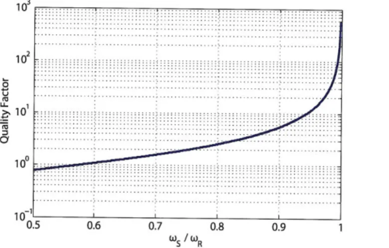
Figure 2.5 presents this relation graphically. Increasing the resonant frequency of the net-work relative to the switching frequency has the effect of increasing the quality factor, but there are negative implications of choosing Or to close to ws. Figure 2.6 plots the value of LR and CR versus Or for a 100 MHz inverter with an input voltage of 5 Volts and an output power of 1 Watt. From this figure it is seen that the components approach extreme values

VHF Converter Architecture

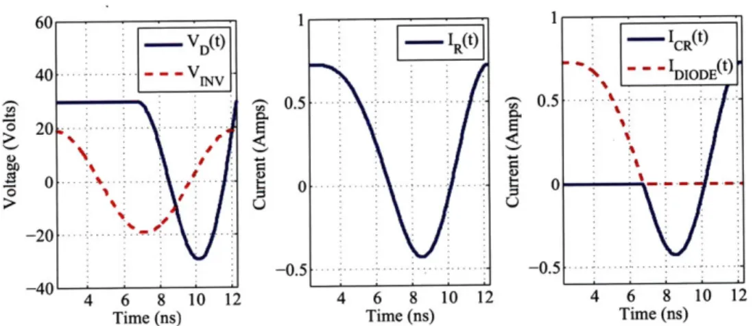
as wr approaches ws. Additionally, the tolerance of the component values becomes very sen-sitive as the slope of the impedance is very steep versus frequency when operating close to resonance. Figure 2.7 shows simulated waveforms using predicted component values from the design solution for the inverter specification previously mentioned and Wr = 0.9 -Ws. The inaccuracy of the design solution can be observed in the waveforms as VD(t) does not achieve perfect zero-voltage-switching. Additionally, both simulated and calculated values of IR(t) are plotted together so the differences can be observed. While not perfect, the design procedure does result with a solution that is quite near to the actual solution. The designer can easily account for this error when simulating the inverter in SPICE.

13

10.

S10' :::..:

Figure 2.5: Plot showing the relation between the quality factor and resonant frequency of the load leg of a class-e inverter

2.1L2 Drawbacks of the Class-E Inverter

While the class-e inverter successfully mitigates switching losses, it has numerous qualities that reduce its usefulness in a practical DC/DC converter circuit. First and foremost the inverter is unable to operate over a wide load range. The quality factor of the output RLC leg of the inverter is set by the load resistance. Thus, the phase shift of load leg is also set by the load resistance since:

Since this phase shift is constrained by the inverter design, the circuit can only be tuned properly for a single load resistance. This phenomena is shown in Figure 2.8 where the load resistance is varied by only a factor of two. Clearly this is an unacceptable condition for a DC/DC converter.

-2.1 The Class-E Inverter

Figure 2.6: Class-e inverter component leg of the inverter

values plotted versus the resonant frequency of the load

V D(t) 0 0. E C U 10 Time (ns) I (t) 10 Time (ns)

Figure 2.7: Simulated class-e inverter waveforms using component values resulting from the design procedure. The inverter is designed for a switching frequency of 100 MHz and an input voltage of 5 Volts. Simulation script is included in Appendix A.

1011 0. 0.6 0.7 0.8 0.9 1 W _SWR 0.7 0.8 S _R .. ......I ... ......: ... ... ... ... ... ... ... ... ... ... ... ... ... . . . .. . . .. . . ... . . . . . . . . . . . . .. . . . . . . . . . . .. . . . . . . . . . . .: . . . . . .. . . .. .... ... .. . . . . ... . . . . . . . . ... . . . . . . . . . . .. . . .. . . .. . . . ... ... ... . . . .. . . . ... . . . .. . . .. . . . . . . . . .. . . . . . . .. . . . . . . . . . . . .. . . .. . . .. .. ... . . . . . . . . .. . . . .. . . ... _{. . . .. . . ...} . . . ._{. . . . . .}. . . . . . ... . . . .... . . .... :- ... ... .. .... .... .. .. . .* .. .. .. .. .. ...* .. ... . ... ... ... ...

.

.

.

.

.

.

.

.

.

.

.

.

.

.

.

.

.

.

.

..

.

.

.

.

.

.

.

.

.

.

.

.

.

.

.

.

.

.

..

.

.

.

.

.

.

.

.

.

.

.

.

.

.

.

.

.

.

...

.

.

.

.

.

.

.

.

..

.

.

.

.

.

.

.

...

.

.

.

.

.

.

.

.

.

VHF Converter Architecture 5- Designed Load --- Decreased Load 40

Figure 2.8: Simulated waveforms of a class-e inverter showing how VD(t) varies with an increased load resistance. Component values are: Lp = 10uH, CE = 67.7pF, CR = 105pF, LR = 34.1nH, and

RLOAD _{is varied from 5 to 10 Ohms. Simulation script is included in Appendix A.}

Furthermore, in a practical design the capacitor CE is partially made up by a parasitic capacitor from the switching device Si. Equation (2.8) can be rearranged to show the following:

POUT= CEIN7ws (2.17)

This shows that the output power is directly proportional to the capacitance of CE. Since this capacitor is partially a parasitic whose value is fixed for a given device, there is a minimum power that the inverter can be designed for.

Finally, the inverter circuit requires a large choke inductor. In the quest for a highly inte-grated DC-DC converter, the requirement for a large inductor is an unattractive prospect, especially if fast dynamic response is sought.

2.2

Class-E DC/DC converter

The class-e inverter is made into a DC/DC converter by replacing the load resistor with a rectifier circuit, as shown in the block diagram of Figure 2.9. Since voltage transformation

-2.2 Class-E DC/DC converter

is done at AC, large conversion ratios can be obtained without extreme duty cycles through the use of a passive transformation network between the inverter and the rectifier [8].

VIN -RLOAD

Figure 2.9: Block diagram of a resonant DC/DC converter

2.2.1 Problems with Hard-Switched Rectifiers

Common hard-switched rectifiers generate a square wave and are not suitable for use in VHF applications. With the very high switching frequency, the harmonics that are generated from the switching waveform easily excite resonances among the parasitics in the circuit leading to oscillations and additional loss. Figure 2.10(a) shows an ideal hard-switched half-wave rectifier circuit driven by a sinusoidal voltage source and loaded by a DC current. When the input sinusoid is positive, D1 is on and carries IDC, and in the second half of the period when the input sinusoid is negative D2 is on and carries IDC -When the input voltage crosses zero, the current must commutate from one diode to the other, resulting in a current square wave. This is troublesome when parasitics are included in the analysis. The dominant parasitics are the junction capacitance of diodes and the series package inductance, shown in Figure 2.10(b). Figure 2.11 shows simulated waveforms of an ideal half-wave rectifier and of a rectifier with parasitics included operating at 100 MHz. With a junction capacitance of 30 pF and a series inductance of 3 nH, the ringing harmonic currents become dominant. This leads to substantial loss since the rectifiers operation is disrupted and the additional harmonic currents do not contribute to delivering power to the load. Additionally, finite commutation time of the diodes brings about the same switching losses that the inverter circuit was specifically designed to avoid.

2.2.2 Resonant Rectifiers

The primary problem facing a hard-switched rectifier for operation at VHF speeds is the parasitic resonant that occurs between the diode's junction capacitance and the parasitic package inductance. In a resonant rectifier, this resonance is used as an advantage rather than a hinderance. The series loaded resonant rectifier of [9], shown in Figure 2.12, is

VHF Converter Architecture

CPAR

'DC VAC

(a) Schematic of an ideal hard-switched half-wave rectifier.

(b) Schematic of a hard-switched half-wave

rectifier including dominant parasitic com-ponents.

Figure 2.10: Hard-switched rectifier circuits

VD(t) Time (ns) IDI(t) Time (ns) ID2(t) 0 5 10 15 20 Time (ns) 25 30 35 40

Figure 2.11: Simulated waveforms of the hard-switched rectifier circuits of Figure 2.10 showing

the effect that including parasitics has on operation at VHF. Simulation performed with VAC = 10

Volts, IDC = 1 Amp, LPAR = 3 nH, and CPAR = 30 pF. Simulation script is included in Appendix A.

- 32 -0

0.

2.2 Class-E DC/DC converter

designed specifically to do this by adding an inductor in series with the diode to control the frequency at which the resonance occurs. To gain a qualitative understanding of how this rectifier operates, it is assumed that the current IR(t) is sinusoidal, and CFILT is large enough such that VOUT is a DC voltage relative to a switching cycle. When the diode turns on, the voltage VD(t) is held at VOUT, and all of the current IR(t) passes through the diode. The diode turns off when IR(t) crosses zero. At this point IR(t) switches to being carried through the diode's parasitic capacitor CPAR . This transition of current from the diode to the capacitor happens without ringing since the current was at zero during the transition. The current IR(t) then charges and discharges CR until the voltage VD(t) reaches VOUT again, turning the diode on and causing the cycle to repeat. At this point, the current in CPAR must transition to the diode, but since this capacitance is physically the same piece of silicon as the diode, this transition occurs without ringing as there is essentially no inductance between them.

- -- _PAR LR LPAR ---.

D,

VAC

Figure 2.12: Schematic of a series loaded resonant rectifier circuit. Note that the AC voltage

source must pass the dc load current.

When using this rectifier circuit with a resonant inverter to build a DC-DC converter, the diode's junction capacitance might not be the needed impedance for proper inverter tuning. An external capacitor can be added in parallel with the diode to fix this problem, shown in Figure 2.13. In doing so, however, the parasitic inductance between this external capacitor and the diode introduces some ringing into the resonant rectifier circuit when the diode turns on. While this is exactly the behavior that the circuit sought to avoid, the outcome in many cases is tolerable as diode's junction capacitance is still being absorbed by the topology. Simulated waveforms comparing of an ideal resonant rectifier, and a rectifier containing the same parasitics of the previously described hard-switched rectifier are shown in Figure 2.14. Resonant boost converter using this rectifier topology have been successfully demonstrated with switching frequencies up to 110 MHz in [10], [11], [12], and [13].

VHF Converter Architecture

VAC

Figure 2.13: Schematic of a series loaded resonant rectifier circuit with extra capacitance for converter tuning and dominant parasitic components included

VD(t)

Time (ns)

ID(t)

5 10 15 20 25 30 35 40

Time (ns)

Figure 2.14: Simulated waveforms from the resonant rectifier of parasitics included. Simulation script is included in Appendix A.

Figure 2.13 both with and without

- 34

--0.1

-0

2.2 Class-E DC/DC converter

2.2.3 DC-DC Converter Topology

Figure 2.15 shows the a schematic of a resonant boost DC-DC converter that is formed by joining together a class-e inverter and a series loaded resonant rectifier. Figure 2.16 presents waveforms from a SPICE simulation of this converter with ideal components. Aside from the output filter capacitor, the dc-dc converter only requires adding a single diode to the class-e inverter circuit, as the output tank of the inverter and the input tank of the rectifier are shared. Also, LR and CR are rearranged relative to the class-e inverter circuit to provide a DC link from input to output. The constrains the converter topology to boost applications only due to the diode's polarity. Note that in this topology there is some direct transfer of energy at DC from the input to the output (unlike the case where all energy flow is mediated through AC waveforms). From simple conservation of energy arguments, it is shown that the ratio of AC to DC power transfer is set by the conversion ratio:

PAC _VouT _{1 (2.18)}

PDC VIN

LF VD(t) LR VRt D, VOUT

IF(t) IR~

VIN S, E CR

CFILT

Figure 2.15: Schematic of a resonant boost DC/DC converter made by joining together a class-e inverter and a series loaded resonant rectifier.

Designing this general type of converter has traditionally be accomplished by repeatedly performing time-domain simulations in SPICE sweeping the available parameters in the circuit until the desired waveforms are achieved [3] and [5]. Since there are closed-form equations describing the class-e inverter alone, typically design starts with an inverter cir-cuit. The inverter design requires a specific current IR(t), and the rectifier has to be designed to provide this current when driven by the inverter. The non-linear nature of the rectifier has traditionally made it difficult to derive a set of closed-form design equations, and its design is usually accomplished in SPICE. By sweeping over values of Wr and ZR it is readily observed that Wr roughly controls the phase of IR(t), and ZR controls the amplitude. Thus, the designer has two control knobs to dial the current to the desired amplitude and phase. In Chapter 3 a new design methodology for this converter circuit is presented that is based

VHF Converter Architecture CU 0 5 10 15 20 Time (ns) 4 0 ..- --. .-. -...-.... .. .. . . .. .. . .. .--- - - ---- .. - -- - - - - V (tW - - -VR(t > % 0 5 10 15 20 Time (ns)

Figure 2.16: Simulated waveforms from the boost converter of Figure 2.15 operating at 100 MHz with an input voltage of 12 Volts and an output voltage of 30 Volts.

on direct analysis of the topology and does not require SPICE simulation sweeps across parameters to determine good designs.

2.2.4 Converter Control

Since this boost converter topology is based on a class-e inverter circuit, it inherits all the associated problems that were previously presented.. Most notably, the converter operation is dependant on the value of the resistor loading the converter. As with the class-e inverter, the converter is only tuned properly and operates with zero-voltage-switching for a specific load resistance. Additionally, as load resistor set the

Q

A control scheme has been designed that allows the converter to operate over a wide load range without losing proper tuning [14], [15], and [16]. This is accomplished by modulating

-2.2 Class-E DC/DC converter -- Designed Load -Decreased Load .. . ... . .... ... .. .. . Resistance -2 4 6 8 10 Time (ns) V R(t) 2 4 6 8 10 Time (ns) V D(t) 12 14 16 18 20 12 14 16 18 20

Figure 2.17: Simulated converter waveforms showing the effect of decreasing the load resistance by a factor of two. Simulation script is included in Appendix A.

the converter on and off at a frequency far below the switching frequency to regulate the average output power. While the converter is on, so long as the output voltage is close to the designed value, the converter operates with the designed maximum power value and is tuned correctly. A capacitor is added in parallel with the load to filter modulation harmonic content, and a feedback controller closes the loop. Figure 2.18 shows a block diagram of this system. This control scheme has been successfully demonstrated in [14], [15], [16], [5], [3], [10], [12], [11], and [13].

]Enab GateVHF Controller Enab Dr vererg

vREF + Converter CFILT RLOAD

Feedback

Figure 2.18: Block diagram of the boost converter control system

This scheme successfully enables the converter to efficiently operate over a wide load range. The speed at which the convertei can be modulated sets the size of the output filtering components. The ability to modulate on and off quickly is in part limited by the inclusion of a large choke inductor in the inverter circuit [3]. This choke inductor causes the inverter to take a long time to reach steady-state. Figure 2.19 demonstrates this by simulating the

CA_ An ... ... . .... .... . .. .. .. . . .. .. . . .. . .. ... .. .. .. .. . ... .. .. . .. .. ... . .. .. .. % % % ... - I . ... ... ... _{... .} % % ... ... ... ... ... . ... ...

VHF Converter Architecture

start-up transient of a 100 MHz converter boosting 12 to 30 Volts with LF=3[tH and 40 nH. This -two order magnitude reduction in inductance results in a dramatically faster start-up transient. The converter does not reach efficient operation until steady-state is achieved, and when designing an on/off control loop, the minimum on time must be a significant fraction larger than the start-up transient such that efficiency is not significantly degraded.

vD(t)

Figure 2.19: Simulated waveforms of the start-up transient from two converter designs, both designed to operate with an input voltage of 12 Volts, an output voltage of 30 Volts, and a switching frequency of 100 MHz. One design uses LF=3 pH and is labeled "Choke Inductor", and the other design uses LF=40 nH and is labeled "Resonant Inductor"

2.2.5 Resonant Input Inductor

The size of inductor LF can be reduced without significantly changing the converter op-eration [17]. _{As the size of LF is reduced it begins to resonate'with the other passive} components in the circuit and carries both AC and DC current. Since the design procedure for the class-e inverter presented earlier in the chapter assumed that LF carries only DC current, the other component values must be adjusted to account for the added AC current. To gain a qualitative understanding of the effect that making LF resonant has on the circuit in steady-state, it is assumed that it only resonates with CE. The schematic of Figure 2.20 shows this by splitting LF into two inductors: LF-DC is a large inductor (approaching

-2.2 Class-E DC/DC converter

CE CR CFILT RLoAD

Figure 2.20: Schematic of the converter circuit used to gain a qualitative understanding of the effects of reducing the size of LF

infinity) that carries DC current and is an open circuit at AC, and LF-AC is the small resonant inductor. At AC, these two hypothetic inductors are in parallel, and since LF-DC is infinitely large, their parallel combination has the value of LF-AC. The parallel combination of LF-AC and CE results in the following impedance at w,:

ZEQ - ,WsLF-AC (2.19)

4 SW2LF-ACCE

To maintain proper converter tuning, this impedance must be the same as the impedance of CE. By equating these impedances, the new value of CE can be found as a function of

the LF-AC:

1 + Ws LF-ACCE (2.20)

CE-NEW = LF'AC

Figure 2.21 presents simulation results of a 100 MHz converter boosting 12 to 30 Volts tuned using this method to have LF=40 nH. The figure shows that the calculated value of CE was not quite right, as the converter does not achieve zero-voltage-switching. This is because the impedance of the parallel combination of LF and CE was only accounted for at the fundamental, and the harmonic content of VD(t) is presented with the incorrect impedance. Luckily, the fix is easy, as the new value of CE is simply reduced until ZVS is achieved. A new design methodology that will be introduced in Chapter 3 fixes this problem and accounts for the impedances exactly.

2.2.6 Mitigation of Frequency Dependent Loss Mechanisms

This section summarizes the technique used to overcome each of the frequency dependent loss mechanisms of a hard-switched converter as introduced in Chapter 1:

VHF Converter Architecture V D(t) 50 45 - - - Calculated - - - Corrected 4 0. ... ... .... .. .. Ia I I '35 . .. ... 0 > 25 . . -. .

~

Figure 2.21: Simulated converter waveforms showing the error in equation (2.20) for a 100 MHz converter with an input voltage of 12 Volts, an output Voltage of 30 Volts, and LF=40 pH. Simulation script is included in Appendix A.

" Switching Loss: The converter architecture is specifically designed to operate with zero-voltage-switching to avoid both overlap loss and capacitive discharge at the switching instants.

" Gating Loss: If a hard-switched gate driver results in too much loss for the operating conditions, a resonant gate driver can be used to recover a portion of the energy stored in the gate, rather than discharging it to ground [1], [16], and [15].

" Magnetic Core Loss: With the frequency dependent device losses minimized, the con-verter can be operated at a frequency high enough that the inductors implemented with either low loss low permeability RF core materials [18] or by removing the core altogether, thus avoiding core-loss.

2.3

Relation to Other Converters

It should be noted that aside from the important aspects of component values and control, the proposed converter circuit of Figure 2.15 is topologically equivalent to the ZVS mul-tiresonant boost converter of [4] and to the resonant boost converter of [3]. The difference in design between the converter of [4] and here is quite large owing to major differences in control (constant on-time variable frequency vs. burst mode control) and the resulting difference in the choice of component values. The design here is more similar to that of [3],

- 40