HAL Id: hal-00095625
https://hal.archives-ouvertes.fr/hal-00095625
Submitted on 2 May 2019
HAL is a multi-disciplinary open access
archive for the deposit and dissemination of
sci-entific research documents, whether they are
pub-lished or not. The documents may come from
teaching and research institutions in France or
abroad, or from public or private research centers.
L’archive ouverte pluridisciplinaire HAL, est
destinée au dépôt et à la diffusion de documents
scientifiques de niveau recherche, publiés ou non,
émanant des établissements d’enseignement et de
recherche français ou étrangers, des laboratoires
publics ou privés.
Impact of Climate Change on the Future Chemical
Composition of the Global Troposphere
Guy Brasseur, Martin Schultz, Claire Granier, Marielle Saunois, Thomas
Diehl, Michael Botzet, Erich Roeckner, Stacy Walters
To cite this version:
Guy Brasseur, Martin Schultz, Claire Granier, Marielle Saunois, Thomas Diehl, et al.. Impact of
Climate Change on the Future Chemical Composition of the Global Troposphere. Journal of Climate,
American Meteorological Society, 2006, 19 (16), pp.3932-3951. �10.1175/JCLI3832.1�. �hal-00095625�
Impact of Climate Change on the Future Chemical Composition of the
Global Troposphere
GUYP. BRASSEUR,* MARTINSCHULTZ, CLAIREGRANIER,⫹ MARIELLESAUNOIS, THOMASDIEHL,# MICHAELBOTZET,AND ERICHROECKNER
Max Planck Institute for Meteorology, Hamburg, Germany
STACYWALTERS
National Center for Atmospheric Research,@ Boulder, Colorado (Manuscript received 25 January 2005, in final form 27 September 2005)
ABSTRACT
A global chemical transport model of the atmosphere [the Model for Ozone and Related Tracers, version 2 (MOZART-2)] driven by prescribed surface emissions and by meteorological fields provided by the ECHAM5/Max Planck Institute Ocean Model (MPI-OM-1) coupled atmosphere–ocean model is used to assess how expected climate changes (2100 versus 2000 periods) should affect the chemical composition of the troposphere. Calculations suggest that ozone changes resulting from climate change only are negative in a large fraction of the troposphere because of enhanced photochemical destruction by water vapor. In the Tropics, increased lightning activity should lead to larger ozone concentrations. The magnitude of the climate-induced ozone changes in the troposphere remains smaller than the changes produced by enhanced anthropogenic emissions when the Special Report on Emission Scenarios (SRES) A2P is adopted to describe the future evolution of these emissions. Predictions depend strongly on future trends in atmo-spheric methane levels, which are not well established. Changes in the emissions of NOx by bacteria in soils and of nonmethane hydrocarbons by vegetation associated with climate change could have a significant impact on future ozone levels.
1. Introduction
The chemical composition of the atmosphere has been changing substantially during the twentieth cen-tury in response to human activities. It is well known, for example, that the concentration of greenhouse gases has increased dramatically since the beginning of the industrial revolution. The atmospheric abundance
of reactive gases, specifically of tropospheric ozone, has also been considerably perturbed, primarily through in-tense emissions of combustion products such as carbon monoxide, nitrogen oxides, and volatile organic com-pounds, specifically in industrialized regions, where large amounts of fossil fuel are burnt, and in the Trop-ics, where biomass burning is frequent. The rapid in-crease in the methane concentration, in response to agricultural activities, has also contributed to enhanced ozone levels in the troposphere. The magnitude of the preindustrial level of ozone is not accurately estab-lished. Early observations made with the widely used Schönbein paper (a test paper impregnated with a mix-ture of potassium iodide and starch, and exposed to the air for several hours) suggest that the surface ozone mixing ratio was as low as 5–20 ppbv at the end of the nineteenth century (Volz and Kley 1988; Anfossi et al. 1991) in most parts of the world, even in continental regions like Europe. However, as highlighted by Pave-lin et al. (1999), the measurements made using Schön-bein’s method were contaminated by the presence of water vapor, and uncertainties in the humidity
correc-* Current affiliation: National Center for Atmospheric Re-search, Boulder, Colorado.
⫹ Additional affiliation: Service d’Ae´ronomie/IPSL, Paris, France, and Aeronomy Laboratory, NOAA–CIRES, Boulder, Colorado.
# Current affiliation: NASA Goddard Space Flight Center, Greenbelt, Maryland.
@ The National Center for Atmospheric Research is sponsored by the National Science Foundation.
Corresponding author address: Guy P. Brasseur, National Cen-ter for Atmospheric Research, P.O. Box 3000, Boulder, CO 80307.
tion have led to considerable inaccuracies in these ozone measurements. Ozone is a greenhouse gas and a powerful oxidant. As a precursor of the hydroxyl (OH) radical, it strongly influences the photochemical life-time of many compounds and hence affects the self-cleaning ability (or oxidizing power) of the atmosphere. Several studies using chemical transport models (see, e.g., Lelieveld and van Dorland 1995; Berntsen et al. 1997, 2000; Brasseur et al. 1998; Wang and Jacob 1998; Stevenson et al. 1998; Mickley et al. 1999; Shindell et al. 2001, 2003; Hauglustaine and Brasseur 2001; Lamarque et al. 2005) have estimated the changes in the concen-tration of tropospheric ozone and the related radiative forcing since the preindustrial era in response to chang-ing emissions of chemical compounds. Model results are summarized in a report recently published by the European Commission (2003). These models have also been used to predict possible future changes based on preestablished emission scenarios (see e.g., van Dor-land et al. 1997; Stevenson et al. 1998, 2000, 2005; Bras-seur et al. 1998; Hauglustaine and BrasBras-seur 2001; Grewe et al. 2001; Prather et al. 2003; Gauss et al. 2003). Several of these models (Stevenson et al. 2000, 2005; Grewe et al. 2001; Zeng and Pyle 2003; Murazaki and Hess 2006) have considered several potential feed-back mechanisms linking future climate changes and ozone, specifically perturbations in the atmospheric cir-culation, temperature, water vapor concentration, cloudiness, etc.
The purpose of the present study is to assess the impact of predicted climate change on the future con-centration of reactive gases in the troposphere, and to compare these climate-generated effects on the atmo-spheric composition with changes resulting directly from increasing chemical emissions. The goal is not to investigate in detail several possible scenarios, based on plausible economic futures, but to show through some specific model sensitivity cases the potential impor-tance of future climate change, when predicting the re-sponse of the atmosphere to enhanced surface emis-sions.
In section 2, we briefly describe the modeling system used in the present study, and in section 3, we present the scenarios adapted to drive the model simulations. In section 4, we analyze and discuss the model results and assess the respective effects of climate change and increased surface emissions on the future chemical composition of the global troposphere. Conclusions are presented in section 5.
2. Description of the model system
To assess the impact of future climate changes on the chemical composition of the atmosphere, we use a
chemical transport model, the Model for Ozone and Related Tracers, version 2 (MOZART-2), which is driven by meteorological fields provided by a three-dimensional climate model. This climate model simu-lates the coupled atmosphere–ocean–ice system and is forced by a 1% yr⫺1increase in the “effective” atmo-spheric CO2concentration. The so-called effective CO2
is assumed to provide a radiative forcing that implicitly includes the contributions of all well-mixed greenhouse gases released to the atmosphere as a result of human activities.
The atmospheric component of the coupled climate model is ECHAM5, the latest version of the ECHAM model (Roeckner et al. 2003, 2006). It is run at T42 spectral resolution, which corresponds to a horizontal resolution of about 2.8°⫻ 2.8° and employs 19 layers in the vertical with the uppermost level located at 10 hPa. The ocean component of the model system is the Max Planck Institute Ocean Model (MPI-OM-1; Marsland et al. 2003). This model component is based on a C-grid version of the Hamburg Ocean Model in Primitive Equations (HOPE) run on a curvilinear grid with equa-torial refinement (⬃10–50 km at high latitudes and near the equator). A Hibler-type dynamic/thermodynamic sea ice model and a river runoff scheme are included in the coupled model. The coupled atmosphere–ocean model does not employ flux adjustments or any other corrections. First results from a 250-yr control experi-ment are discussed by Latif et al. (2004).
The atmospheric dynamical fields provided by the coupled ECHAM-5/MPI-OM-1 model are archived for a period of 10 yr corresponding approximately to present-time levels of CO2(370 ppmv) and to twice this
value (740 ppmv), respectively. The second case is as-sumed to be representative of the climate to be ex-pected around year 2100.
The chemical transport model used to simulate the chemical composition of the troposphere and the lower stratosphere is the MOZART-2 model, which is de-scribed in detail by Horowitz et al. (2003). The model (version 2.1) is integrated on a grid at a latitudinal and longitudinal resolution of 2.8° and with 19 levels in the vertical up to 10 hPa. It includes a chemical scheme for the ozone/nitrogen oxides/hydrocarbon system that in-volves 63 species and 170 reactions. The chemical sys-tem is solved with a 20-min time step, using a fully implicit Euler backward method with Newton– Raphson iteration. As indicated by Horowitz et al. (2003), the concentrations of several compounds in-cluding ozone, nitrogen oxides, and nitric acid are con-strained above the thermal tropopause by relaxation toward specified zonally and monthly averaged values (relaxation time constant of 10 days). With this model
setup, the accuracy of the calculated changes in cross-tropopause fluxes is limited. More reliable results should be obtained from a model such as MOZART-3 (Kinnison et al. 2006, manuscript submitted to J.
Geo-phys. Res.) in which the concentrations of all chemical
species are calculated in the middle atmosphere. Sur-face emissions include fossil fuel combustion, biomass burning, biogenic processes related to vegetation and soils, and exchanges with the ocean. NOx production by lightning is distributed depending on the location of convective clouds as diagnosed by MOZART-2. The flash frequency is estimated according to Price and Rind (1993). Tracer advection is performed using the flux form semi-Lagrangian finite-volume algorithm de-veloped by Lin and Rood (1996). Convective transport is based on the parameterization of Zhang and McFar-land (1995) for deep convection and of Hack (1994) for shallow convection. Vertical exchanges in the boundary layer are parameterized according to Holtslag and Bo-ville (1993). Advection, convective transport, boundary layer mixing, cloudiness, and precipitation as well as wet and dry deposition, are derived in MOZART-2, using the formulations adopted in the Model for Atmo-spheric Transport and Chemistry (MATCH; Rasch et al. 1997) with input variables (zonal and meridional winds, temperature, specific humidity, surface pressure, and surface fluxes of heat and momentum) provided by the ECHAM model with a time interval of 6 h. Note therefore that the representation of unresolved physical processes in MOZART is not entirely consistent with the formulation of the same processes adopted in the ECHAM model. It should also be realized that the
model setting adopted here is not providing a full two-way coupling between atmospheric dynamics and chemistry because the calculated distributions of radia-tively active species like ozone calculated by MOZART do not feed back into ECHAM. The one-way coupling realized in the present study allows us, however, to iso-late specific processes, perform sensitivity tests, and hence understand the nature and magnitude of the cou-pling. But by adopting this approach, it is therefore assumed that tropospheric ozone has little influence on climate compared to other effects (water feedback, aerosol/cloud effects, etc.).
The atmospheric distributions of chemical species provided by MOZART-2 were evaluated in detail in the study by Horowitz et al. (2003). This paper shows that the distributions of most chemical species are well reproduced by the model with a few limited exceptions. For example, MOZART-2 tends to overestimate the concentration of ozone and peroxyacetyl nitrate (PAN) near the tropopause at higher northern latitudes, and to underestimate the concentration of carbon monoxide at some observation sites of the Northern Hemisphere.
3. Scenarios
To assess the impact of increasing emissions of chemical compounds and of climate changes on the chemical composition of the atmosphere, we consider nine different cases (Table 1). For each of them, the MOZART model is integrated for a period of 10 yr. The first year is discarded to allow for the spinup of the model. The 9-yr average fields are computed for each month of the year.
TABLE1. Scenarios considered in the present study.
Case Year for anthropogenic emissions Aircraft emissions (TgN yr⫺1) Methane
(ppmv) Other emissions Climate
Calculated tropospheric
O3column
(DU) Remarks A 2000 0.7 1.7 Baseline 1⫻CO2 29.75 Baseline (reference) case
P 1890 None 0.85 Baseline 1⫻CO2 20.59 Preindustrial (1890)
B 2000 0.7 1.7 Baseline 2⫻CO2 31.31 Baseline with future climate
(2100)
C 2100 0.7 3.6 Baseline 1⫻CO2 Future scenario with present
climate
D 2100 2.92 3.6 Baseline 1⫻CO2 43.72 Same as C, but with increased
aircraft emissions E 2100 2.92 3.6 Baseline 2⫻CO2 44.34 Future scenario with future
climate
F 2100 2.92 1.7 Baseline 2⫻CO2 39.49 Methane does not increase in the
future G 2100 2.92 3.6 Isoprene and soil NO
emissions⫻ 2
2⫻CO2 46.62 Impact of climatically changed
vegetation and soil emissions H 2100 2.92 3.6 Biomass burning⫻ 2 2⫻CO2 41.88 Impact of biomass burning
Case A, the baseline case, refers to the current at-mosphere (approximately year 2000) and is used as the reference case. The emissions of chemical compounds are those adopted in Houghton et al. (2001) and de-scribed in the paper by Prather et al. (2003) and Gauss et al. (2003). The corresponding global emissions of CO and NOx are listed in Table 2. The tropospheric mean mixing ratio of methane is approximately 1.7 ppmv with surface values fixed as monthly averages based on ob-servations (GLOBALVIEW-CH4 2001).
In simulation P, the emissions of chemical com-pounds are scaled to be representative of the preindus-trial era (year 1890). Natural emissions are identical to those adopted for the present-day simulations. In the case of anthropogenic contributions, the emissions re-lated to road and nonroad traffic are assumed to be zero, while industrial emissions are specified as 15% of the present-day values (same spatial distribution). This assumption accounts for the fact that industrialization started before 1890 in several countries of the Northern Hemisphere. Biomass burning emissions, which are of-ten related to human activities, are prescribed to be 20% of the present emissions in the case of savanna fires, and they are equal to zero in the case of tropical forest fires (since deforestation was not prominent at that time). Emissions associated with forest fires at mid-and high latitudes, which are partly of human origin, are assumed to be a factor of 2 lower than present emissions. The level of methane adopted for the 1890 simulation is equal to 0.85 ppmv. Note, that for this particular scenario, the dynamics of the atmosphere provided by the ECHAM-5/OM-1 model is the same as in case A.
In case B, the emissions are identical to those model run A, but the climate as derived from the ECHAM-5/OM-1 model corresponds to a situation representa-tive of a 10-yr period close to year 2100. This specific case allows us to isolate the effect of expected climate change (change in temperature, water vapor abun-dance, convective activity, lightning distribution and frequency, and precipitation rate) on the chemical com-position.
In case C, the surface emissions are modified to be representative of year 2100 on the basis of the A2P scenario used in Houghton et al. (2001). This scenario is an adaptation for reactive species of the A2 scenario developed by the Special Report on Emission Scenarios (SRES) for greenhouse gases (I. S. A. Isaksen 2005, personal communication). The A2 scenario corre-sponds to a very heterogeneous world in which coop-eration between the different countries is limited, and progress toward clean technologies is slow. The world population increases rapidly to reach 15 billion in year 2100, and the income per capita is lower than in the other SRES scenarios. In case C, the emissions from aircraft engines remain unchanged from the reference level (year 2000), and the climate variables are those of the baseline case (year 2000). The A2P scenario, which provides considerable perturbations, is adopted here not because it represents the most probable case, but because it facilitates the identification of the potentially important processes that link climate changes and air quality at the global scale. Figure 1 shows the total emissions of CO and NOx established on a 1°⫻ 1° grid for years 1890, 2000, and 2100, respectively. The regions most affected by changes in the emissions are Europe and North America for the 1890–2000 period, and Asia and South America for the 2000–2100 period. Under the adopted scenario, the anthropogenic emissions of CO increase by a factor of 8 between 1890 and 2000 and 2.5 between 2000 and 2100. The corresponding values for the NOx increase are 16 and 3, respectively. Bio-mass burning emissions are assumed to be unchanged after year 2000.
Case D is identical to case C, but with enhanced aircraft emissions. As no reliable predictions for these emissions exist for year 2100, the values adopted here are those of year 2000 multiplied by a factor of 4, with the same spatial distribution as present day. Under these assumptions, the total NOx emission by aircraft represents 2.9 Tg yr⫺1against 0.7 TgN yr⫺1under base-line conditions. More accurate information would require reliable estimates of the aircraft fleet size, the type of engines, and the extent and geographical distribution of fleet operations to be expected in year 2100. The values adopted here provide no more than a crude way to
TABLE2. Emissions for preindustrial, present, and future
conditions adopted in the model.
Year Anthropogenic Biomass burning Biogenic emissions Oceans Total CO (TgCO yr⫺1) 1890 84 65 160 20 329 2000 650 337 160 20 1167 2100 1680 337 160 20 2197 NOx (TgN yr⫺1) 1890 1.5 1.4 2.9 — 6.8 2000 31.8 6.2 8 — 46.0 2100 109.0 6.2 8 — 123.2 C2H6(TgC yr⫺1) 1890 0.5 0.3 0.8 0.8 2.4 2000 5.5 2.0 0.8 0.8 9.1 2100 11.0 2.0 0.8 0.8 14.6 C2H4(TgC yr⫺1) 1890 1.1 0.7 4.3 1.2 7.2 2000 3.9 4.1 4.3 1.2 13.5 2100 7.8 4.1 4.3 1.2 17.4
assess the sensitivity of enhanced aircraft operations on the concentration of tropospheric trace species.
Case E corresponds to the same situation as case D (2100 emissions), but with climate conditions represen-tative of year 2100 (doubled equivalent CO2 level).
Thus, case E accounts simultaneously for the impacts of
future anthropogenic emissions under scenario A2P and for the climate change calculated for a period around year 2100 by the Hamburg Climate System Model.
A major uncertainty in the prediction of the atmo-spheric composition is the future trend in the methane
FIG. 1. Surface emissions (cm⫺2s⫺1) of carbon monoxide (CO) and nitrogen oxides (NOx) in July corresponding to the years (left) 1890, (middle) 2000, and (right) 2100, respectively.
concentrations. During the 1980s, trends of typically 1% yr⫺1were reported on the basis of surface obser-vations (Dlugokencky et al. 1994). The trends have been substantially lower in the 1990s and have even become insignificant in the last years. The changes in observed trends are not fully explained at present, so that any prediction for the future is difficult. Based on the adopted scenario, the mixing ratio of methane should reach approximately 3.6 ppmv (global average surface value), which is slightly more than a factor of 2 increase compared to the year 2000 values (average of 1.7 ppmv). To assess the importance of this uncertainty, we have also considered a “minimum” case (case F), in which the methane abundance remains at the year 2000 level, while all other forcings are similar to case E (in-cluding a doubling in the atmospheric concentration of equivalent CO2).
Finally, we have investigated the impact of other potential changes, which could result from climate changes and are not accounted for in the previous model runs. In case G, we make a sensitivity test to account for climate-driven changes in the temperature-dependent emissions of isoprene by vegetation and of nitrogen oxides by soils. These potential indirect effects are not yet well quantified. Therefore, in this particular model case, the isoprene and soil NOx emissions have been uniformly doubled in year 2100. Ongoing work suggests that this factor may not be unrealistic in the case of isoprene emissions (C. Wiedinmyer et al. 2005, personal communication). In the case of soil NO, Yienger and Levy (1995) indicate that the emissions are increasing with temperature, especially in the case of wet soils. More detailed work is needed to provide more accurate estimates as well as the geographical and seasonal dependence of these expected changes. Other imposed changes are the same as those adopted in case E.
The consequences of future climate changes on wild-fires are currently unknown, but could be substantial. The vulnerability of the forests to fires could increase in a warmer climate, although this effect may be transient and different in different parts of the world. In case H, we performed a sensitivity test in which the emissions by biomass burning are increased uniformly by a factor of 2, while the other forcing parameters are identical to those adopted in case E.
4. Model results
a. The baseline case (A)
To evaluate the global distributions of reactive gases provided by the MOZART–ECHAM–OM model sys-tem, we first present distributions of chemical species
obtained for the baseline conditions (case A). Figure 2 shows the zonally and monthly mean distributions of carbon monoxide (CO) and ozone (O3) calculated for
January (left) and July (right). In the case of CO, the zonally averaged mixing ratios are always higher in the Northern Hemisphere with a maximum in the bound-ary layer located between 30° and 60°N. The CO abun-dances are highest in winter with surface values of typi-cally 180 ppbv at 50°N, to be compared to the 120 ppbv calculated at the same location in summer. In the free troposphere, Northern Hemisphere winter values are decreasing from about 140 ppbv at the top of the plan-etary boundary layer (PBL) to 75 ppbv at 10-km alti-tude. During summer, as vertical mixing is intense, the CO mixing ratio is more spatially uniform, with values ranging from 90 ppbv at the top of the PBL to 60 ppbv at 10 km. Southern Hemisphere free tropospheric val-ues (50°S) are close to 50 ppbv in both seasons.
Ozone is characterized by values decreasing gradu-ally from the stratosphere to the surface. In the free troposphere, during all seasons, minimum mixing ratio values are found in the Tropics where vertical transport of ozone-poor air from the surface affects all levels up to 14 km. Maximum values are derived by the model in the subtropics, where intrusions of stratospheric ozone-rich air and downward motions tend to enhance the tropospheric ozone concentrations. This maximum is highest in the Northern Hemisphere where additional photochemical production associated with the rela-tively high levels of ozone precursors is taking place. In January, the zonally averaged extratropical ozone mix-ing ratio in the 1–5-km layer ranges from 30 to 50 ppbv in the Northern Hemisphere and from 10–30 ppbv in the Southern Hemisphere. In July, the corresponding values are 40–60 and 25–30 ppbv in the Northern and Southern Hemispheres, respectively.
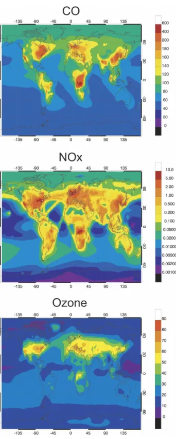
Especially for short-lived species such as NOx, zon-ally averaged values do not provide a useful picture of the spatial distribution of tropospheric species. Large geographical differences primarily associated with the distribution of emissions exist and are illustrated in Fig. 3. This graph displays the surface distribution of monthly mean NOx, CO, and ozone mixing ratios for the month of July. In the case of NOx, the mixing ratio, which is lower than 50 pptv in most oceanic regions, reaches more than 10 ppbv in geographic areas where the use of fossil fuels is high and biomass activity is intense. Hot spots of NOx concentrations are found in the eastern United States, in northern Europe, and in East Asia. High values are also predicted in central Africa. The level of NOx decreases rapidly away from the continental zones even though a substantial en-hancement is found along ship tracks. In the free
tro-posphere (i.e., 5 km; not shown), NOx mixing ratios larger than 100 pptv are found over industrial areas of the United States and in India and China, where con-vective transport and lightning-related production of NOx are intense during certain periods of the year. Outside these areas, midtropospheric NOx mixing ra-tios are typically 20–40 pptv and are determined by the interplay between long-range transported NOx from convective regions (uplift of boundary layer NOx and in situ lightning production), photochemical equilib-rium between NOx and HNO3, and the formation and
destruction rates of PAN.
In the case of CO, whose lifetime is considerably longer than that of NOx, the distribution is spread far-ther away from the major source areas. The calculated surface mixing ratios are highest over the continents, although a plume of CO-rich air originating in North America is visible over the Atlantic Ocean. Surface mixing ratios reach typically 100–150 ppbv in the sum-mer Northern Hemisphere with peaks of several hun-dreds of ppbv in a few spots affected by intense indus-trial activity, transport, and biomass burning. In the
Northern Hemisphere during winter (not shown), the surface CO mixing ratio is of the order of 120–200 ppbv outside the industrial hot spots.
Finally, in the case of ozone, the model provides a surface distribution characterized by summertime mix-ing ratios that are higher than 50 ppbv in North America, Europe, and Asia, and less than 30 ppbv over the oceans (less than 15 ppbv over the tropical ocean). Elevated boundary layer ozone concentrations are cal-culated over the North Atlantic Ocean as a result of a westerly flow from North America and easterly trans-port of pollutants from Europe. In January, when the photochemical production of ozone is relatively weak north of 40°N, the highest surface ozone mixing ratios are found in the subtropical band (20°–40°N) of the Northern Hemisphere, with the highest values being predicted over the ocean where ozone deposition is smallest. Ozone plumes originating from the regions of the Caribbean and eastern China are propagating over the North Atlantic and Pacific, respectively. The impact of biomass burning is also visible in Africa and to a lesser extent in South America and Indonesia.
FIG. 2. Zonally averaged and monthly mean distributions of present-day (year 2000) carbon monoxide and ozone mixing ratios
b. Changes since the preindustrial era
To provide a reference to which current and future changes in the chemical composition of the atmosphere can be compared, we first consider conditions
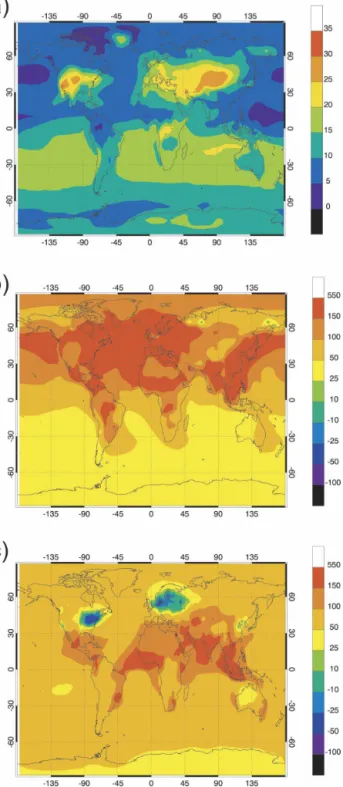
represen-tative of the preindustrial era (year 1890). The assump-tions made for this simulation are provided in section 3 (case P). As can be seen in Fig. 4a, the surface mixing ratio of ozone in July is generally of the order of 5–20 ppbv in all regions of the world, with values somewhat higher in the Southern (winter) than in the Northern (summer) Hemisphere. Values of 10–20 ppbv are cal-culated during July in Europe, the eastern United States, northern and southern Africa, and Australia, in general agreement with the concentrations measured at the end of the nineteenth century and reported by Pavelin et al. (1999). Surface mixing ratios slightly lower than 10 ppbv are calculated in the region of the Sahara, in the northern part of South America and in Japan. The values exceeding 20 ppbv over the North American and Asian continents reflect the influence of NOx emissions by the soils and the low deposition ve-locities in arid or semiarid continental regions. In the Northern Hemisphere, the calculated increase in sur-face ozone between years 1890 and 2000 is of the order of a factor 2 during July (Fig. 4b), except in industrial-ized and urbanindustrial-ized areas, where it reaches a factor of 4 or even 5 (more than 30 ppbv). In addition, the con-centration of boundary layer ozone transported over the North Atlantic Ocean has increased by a factor of 3–4 (more than 20 ppbv). In January (Fig. 4c), the cal-culated Northern Hemispheric surface ozone concen-tration increases by 50%–100% (10–20 ppbv) over the oceans and is multiplied by a factor of 2–3 over the continents, except over highly polluted areas, where it is reduced (10%–50%) through titration by NOx, whose concentrations are particularly high in these re-gions during wintertime. In the Southern Hemisphere, the ozone mixing ratio increases by 30%–75% over the oceans between 1890 and 2000. Above the continents, the calculated increase over the same period is typically 5–10 ppbv or 50%–150% in July. The global annual mean ozone column abundance increases from 21 to 30 Dobson Units (DUs).
The calculated change in the oxidizing power of the atmosphere [as measured by the mean tropospheric loss of methane by the hydroxyl (OH) radical] is rather limited between 1890 and 2000 in the present model simulation in spite of substantial changes in the emis-sions of ozone precursors and in the atmospheric abun-dance of methane. The globally averaged lifetime of methane, calculated below the surface pressure of 200 hPa, and used here as a measure of the oxidizing power of the troposphere, is reduced from 7.7 yr in 1890 to 7.5 yr in 2000. Note that, when performing the calculation up to the tropopause level (rather than the 200-hPa pressure level), Horowitz et al. (2003) report a methane lifetime of 9.4 yr for present-day conditions.
FIG. 3. Monthly mean present-day surface mixing ratio (ppbv) of carbon monoxide, nitrogen oxides, and ozone calculated for July (case A).
c. Future changes in tropospheric composition
In the present section, we assess the changes to be expected in the chemical composition of the tropo-sphere between the 2000 and 2100 periods, assuming
that the emissions are changing according to scenario A2P, as described in section 3. The results presented here are not obtained from a transient integration over time, but are based on “snapshot” calculations: as stated above, the MOZART model is integrated over a period of 10 yr with 10 yr of dynamical evolution taken from the ECHAM5/OM-1 model and representative of periods close to years 2000 and 2100, respectively. Dif-ferent conditions are considered.
1) EMISSIONS OF2100,CLIMATE OF2000 (CASED)
MOZART is integrated using chemical emissions representative of year 2100. The tropospheric mixing ratio of methane is fixed at the surface at 3.6 ppbv, that is, about twice the value observed in year 2000. At each grid point of the model, the emissions by commercial aircraft engines are assumed to be 4 times larger than in year 2000. An additional simulation (case C) in which the aircraft emissions remain unchanged from their present values is also considered. The difference be-tween cases D and C provides an estimate of the effects of quadrupling the current aircraft emissions. In the present simulation, climatic and meteorological con-ditions are the same as for the year 2000 simulation. See section 3 for a description of the adopted emis-sions.
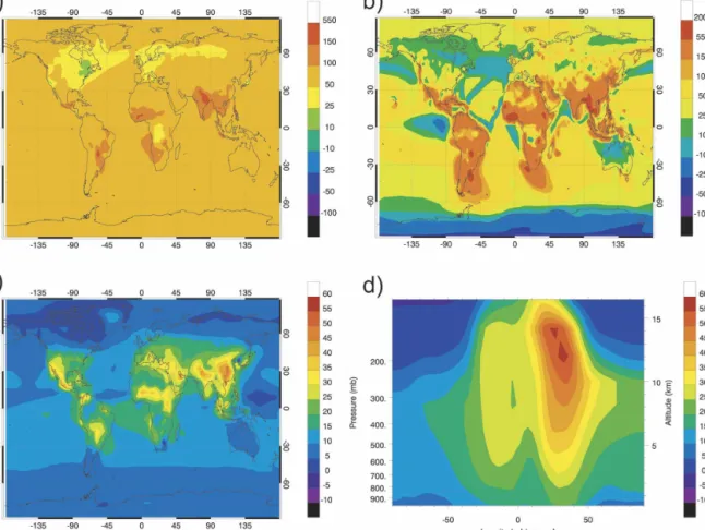
Figure 5a displays the relative change in the surface mixing ratio of carbon monoxide for July conditions. In remote areas far away from the spot sources, CO con-centrations are enhanced by about 70%–90% between years 2000 and 2100, when the A2P scenario is adopted. In areas of high urban and industrial development (South Asia and South America), as well as in Africa, increases of more than 100% are predicted. Changes are considerably smaller in the regions affected primar-ily by North American and European emissions; they are typically 20%–50%. In the free troposphere (not shown), changes are predicted to be of the order of 60%–70% in the Northern Hemisphere and 80% in the Southern Hemisphere.
In the case of NOx (Fig. 5b), the largest changes in the surface concentrations are located in the vicinity of the urban development zones (especially in the Tropics and Southern Hemisphere) with little dispersion far away from the sources. In the free troposphere (not shown), the perturbations are spread over larger dis-tances, and average changes of typically 50%–80% oc-cur in the tropical and subtropical regions.
Between years 2000 and 2100, the average change in the zonally averaged ozone concentration for scenario A2P is of the order of 75% near the equator, and larger than 50% everywhere in the Tropics at all altitudes
FIG. 4. Monthly mean ozone mixing ratio (a) calculated for preindustrial (1890) conditions (case P) in July (expressed in ppbv). Relative change (percent) between 1890 and 2000 in the surface ozone mixing ratio for (b) July and (c) January conditions (case A⫺ case P).
between the surface and the upper troposphere (all sea-sons). In July, changes the extratropics for the same period are estimated to be of the order of 35%–40% in the Northern Hemisphere and 40%–45% in the South-ern Hemisphere. Expressed as mixing ratios, the calcu-lated changes are of the order of 25–30 ppbv near the equator (middle and upper troposphere). They reach slightly more than 50 ppbv at 20°–40°N between 10 and 15 km in July, and slightly more than 35 ppbv at 10°– 30°S in January. These changes derived for fixed ozone levels in the stratosphere are consistent with the varia-tions projected for the same scenario by most of the 11 chemical transport models, and reported by Gauss et al. (2003).
At the surface (Fig. 5c), the largest ozone increase in July (more than a doubling of current values) is pre-dicted for South Asia (India, southern China, and the Indo-Chinese peninsula). In Europe and North America, surface ozone increases by 35%–50% and 10%–25%, respectively. Monthly mean mixing ratios (July) at the surface reach more than 80 ppbv in large parts of California, China, northern India,
and the Middle East (not shown). They become larger than 50 ppbv over the entire North American, Euro-pean, and Asian continents south of 55°N. On an an-nual basis, the changes in the surface mixing ratios are larger than 10 ppbv over the continents in the Tropics and reach more than 25 ppbv in western Mexico and the center of Brazil and of Africa as well as in the region of the Persian Gulf, India, and Southeast Asia. Changes of more than 35 ppbv are projected in parts of southern Asia. Over the oceans, the ozone increase is less than 10 pptv except in a zonal band around 30°N, where it slightly exceeds this value. The calculated changes in the annually averaged ozone changes at the surface, including the geographical patterns, are in good agreement with the values derived by Prather et al. (2003) from the predictions of 10 models following the same scenario.
Finally, the calculations show that, for the A2P sce-nario, the oxidizing power of the atmosphere decreases slightly during the next century (assuming no climate change) with the calculated methane lifetime increasing from 7.5 yr in 2000 to 7.9 yr in 2100.
FIG. 5. Relative change (percent) in the monthly mean (July) surface concentration of (a) carbon monoxide, (b) nitrogen oxides, and (c) ozone, as well as (d) in the zonal mean zone concentration, between years 2000 and 2100 under the A2P scenario and for unchanged climate conditions (case D⫺ case A).
2) EMISSIONS OF2100,CLIMATE OF2100 (CASEE) The assumptions made for case E are similar to the conditions described in the previous section (case D), except that the changes in climate predicted by the ECHAM5/OM-1 model between years 2000 and 2100 are also taken into account. The change in climate manifests itself through changes in tropospheric tem-perature, water vapor abundance, circulation, cloudi-ness, convective activity, lightning frequency, and precipitation rates. To characterize the 2100 climate generated by the ECAHM5/OM-1 model, Table 3 pre-sents the globally averaged temperature and water va-por mass mixing ratios at selected atmospheric levels, and the changes predicted between 2000 and 2100 for January and July, respectively. These values should be compared with the similar calculations performed with the Second Hadley Centre Atmospheric Model (HadAM2b; Johnson et al. 1999). The changes in the zonal mean temperature and water vapor (July) are shown in Figs. 6a,b. Precipitation is also modified in 2100 when compared to present-day (Fig. 6c). In July, for example, convective rainfall increases in the mon-soon region of South Asia and in the western tropical Pacific, while precipitation decrease in the tropical At-lantic and in the eastern Pacific. Such changes affect the removal rate of soluble species such as nitric acid and hydrogen peroxide.
The sensitivity of lightning frequency and intensity to climate change is not well established. Price and Rind (1994) derive from their climate model a 5%–6% in-crease in global lightning activity per kelvin global warming, and hence an equivalent number for the re-lated NOx production. Grenfell et al. (2003) find that the NOx production increases from 4.9 to 6.9 TgN yr⫺1 for a warming of 3.25 K (2100–2000), which cor-responds to a sensitivity of 0.61 TgN yr⫺1 K⫺1 of
12% K⫺1. Grewe et al. (2002) report a rather small signal [5.4 to 5.6 TgN yr⫺1from 1992 to 2015 with cli-mate change according to the Intergovernmental Panel on Climate Change (IPCC) IS92a scenario]. Stevenson
TABLE3. Globally averaged temperature (K) and water vapor mass mixing ratio (10–3 kg kg⫺1) corresponding to year 2000, and the changes (in the same units) predicted for year 2100. Model level (hPa) Temp Temp change Water mass ratio (10⫺3) Change in mass ratio (10⫺3) January 190 213.9 ⫹2.8 0.02 ⫹0.01 320 235.0 ⫹3.2 0.24 ⫹0.10 590 263.8 ⫹2.4 1.94 ⫹0.40 850 278.2 ⫹2.2 5.78 ⫹0.81 July 190 214.6 ⫹3.5 0.03 ⫹0.02 320 237.5 ⫹4.0 0.31 ⫹016 590 266.5 ⫹2.8 2.41 ⫹0.54 850 281.6 ⫹2.3 6.73 ⫹1.11
FIG. 6. Changes in the zonally averaged monthly mean (July) (top) temperature (K) and (middle) water vapor concentration (percent) resulting from climate changes (doubling of CO2level)
as calculated the ECHAM5/OM-1 coupled atmosphere–ocean model (case B⫺ case A). (bottom) Change in the precipitation rate (mm day⫺1) for the corresponding cases.
et
al. (2005) report no significant trend in the global mag-nitude of lightning NOx emissions in their coupled cli-mate chemistry model experiments performed for the 1990–2030 period under the IS92a scenario. They ob-serve, however, some shifts in the distribution of the lightning, including a significant reduction in the Trop-ics below 10 km and an increase at higher levels reflect-ing reduced, but deeper convection. Figure 7 shows the change between 2000 and 2100 in the monthly mean globally integrated NOx production from lightning de-rived in MOZART as a result of changing climate. An increase of approximately 20% is predicted globally, even though changes can be much larger locally. This corresponds to a sensitivity of approximately 9% K⫺1. It should be noted that the lightning parameterization adopted in MOZART is based on cloud-top heights (Price and Rind 1993), which is used as a surrogate for convective activity. Thus, the results obtained here should be regarded as a simple sensitivity study rather than a quantitative prediction.
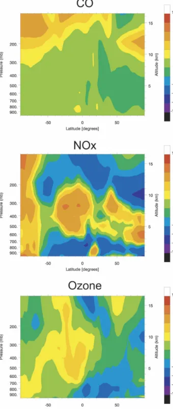
Rather than displaying the overall calculated changes (case E – case A) in the concentrations of chemical species (which resemble those shown in Fig. 5, but with slightly different values), we will show the changes pro-duced only by the changes in climate for the period 2000–2100 (case E – case D). Figure 8 shows the cli-mate-driven change in the zonal mean concentration of CO, NOx, and O3(July average). The largest drivers
associated with climate change are the changes in the background water vapor abundance and in the light-ning-related NOx sources. As indicated by Fig. 6b, the
FIG. 7. Global production of NOx (TgN yr⫺1) by lightning for different months of the year calculated for conditions represen-tative of years 2000 (CO2 ⫽ 370 ppmv) and 2100 (CO2 ⫽ 740
ppmv), and using the Price and Rind (1993) parameterization. The changes in meteorological conditions are those estimated by the ECHAM5/OM-1 climate model for a doubling of atmospheric CO2concentrations.
FIG. 8. Relative change (percent) in the monthly mean (July) zonally averaged concentration of (a) carbon monoxide, (b) ni-trogen oxides, and (c) ozone due to changes in climate conditions for the years 2000 and 2100 (doubling in equivalent CO2
concen-tration) as estimated by the ECHAM5/OM-1 climate model (case E⫺ case D).
water vapor mixing ratio (zonal mean for July) in-creases by as much as 100% in the tropical upper tro-posphere. In the extratropical regions between 5 and 15 km, it increases by 30%–70% in the summer (northern) hemisphere and by 20%–40% in the winter (southern) hemisphere. In the case of NOx, substantial concentra-tion increases (10%–30%) are predicted in the upper levels of the Tropics and summertime extratropics in response to enhanced lightning activity and, in addition, to faster decomposition of PAN. The OH concentra-tions are generally enhanced in response to increased water vapor and NOx abundances. The climate-induced change in the concentration of CO is limited because both the atmospheric production (hydrocarbon oxidation) and the destruction of this compound are proportional to the OH level. In response to climate change, the zonal mean ozone concentration decreases by approximately 5%–10% in the extratropical summer hemisphere, primarily because of the enhanced levels of water vapor. In the Tropics, it increases by 5%–10% because of elevated NOx production by lightning. The small ozone increase of 2%–3% in the Southern Hemi-sphere (winter; low photochemical activity) is attrib-uted to the transport of tropical air masses with en-hanced ozone concentrations.
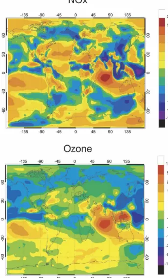
Figure 9a shows that the changes in NOx at 500 hPa resulting from climate change only are quite irregular in space, because they are associated with changes in the geographic location of convective regions as predicted by the ECHAM–OM climate model. The changes in the midtropospheric ozone concentration (Fig. 9b) fol-low those of NOx, with several spots in the vicinity of enhanced lightning areas. Away from these spots, the ozone concentration generally decreases.
The lifetime of methane, which is used as a surrogate for the oxidizing power of the atmosphere, is also af-fected by climate change. Our calculations suggest that the introduction of the climate change effects in the model simulation reduce the lifetime of methane by approximately 0.8 yr. Thus, this climate feedback effect is expected to reduce the atmospheric concentration of CH4, and hence reduce climate forcing produced by this
chemical compound.
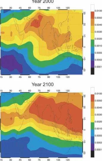
An interesting feature noted in the NOx and ozone changes during July, and associated with the climate-related perturbations, is the large increase predicted for the abundance of these compounds over the Indian Ocean in the vicinity of the equator. This particular feature is attributed to changes in the July circulation that are predicted in this region by the ECHAM–OM model. As shown in Fig. 10, the shape of the dynamical barrier (9-yr average) for water vapor changes from a wavy structure in year 2000 to a more zonally uniform
shape in 2100. Changes in the concentration of ozone and other compounds in the vicinity of such a particular event can be very large. The dynamics of the tropo-pause region is also somewhat modified as a result of climate change. With the assumptions adopted here, the mean height of the tropical tropopause increases by approximately 600 m between years 2000 and 2100. The meridional circulation is slightly enhanced, leading, for example, to a small increase (about 1%) in the methane mixing ratio in the tropical lower stratosphere, and an equivalent decrease in the extratropical upper tropo-sphere.
Finally, it should be stressed that the differences in the chemical fields resulting from climate change shown here for chemical emissions representative of year 2100
FIG. 9. Relative change (percent) in the monthly mean (July) concentration of (a) nitrogen oxides and (b) ozone at 500 hPa due to changes in climate conditions for the years 2000 and 2100 (dou-bling in equivalent CO2 concentration) as estimated by the
(case E⫺ case D) are not significantly different from the similar differences calculated for chemical emis-sions at their year 2000 level (case B⫺ case A). Both cases highlight the indirect effects of a CO2doubling on
the concentrations of ozone and other chemical com-pounds through changes in atmospheric temperature, water vapor concentrations, and dynamics.
3) IMPACT OF METHANE TRENDS
Crutzen (1988), Thompson et al. (1992), and more recently Fiore et al. (2002) have highlighted the impor-tance of methane to background tropospheric ozone. Since the recent trends observed in atmospheric meth-ane are not well understood, and consequently future trends are highly uncertain, it is important to assess the impact of future methane scenarios on calculated ozone (Fiore et al. 2002). The results presented above (see,
e.g., Fig. 5) assume a relatively large increase in the methane mixing ratio during the twenty-first century (from 1.7 ppmv in year 2000 to 3.6 ppmv in 2100). We also consider an additional scenario (case F), in which the methane level in 2100 remains the same as in 2000 (no methane trend). The emissions of other compounds follow the A2P scenario as above, and the “equivalent” CO2level is assumed to double during the twenty-first
century as in case E. Note a slight inconsistency in this assumption since the lack of methane trend should slightly reduce the growth in the equivalent CO2
forc-ing. However, as we are performing a sensitivity case to assess the photochemical role of methane, all other fac-tors are maintained as in the previous case. Figures 11a,b compare the changes in the zonally averaged ozone concentrations when the methane trend is in-cluded (case E) and when it is ignored (case F). The difference in the zonal ozone average concentration in the Tropics is close to 20% between these two sce-narios. The difference associated with the uncertainty in the future
FIG. 10. Water vapor volume mixing ratio (500 hPa) over the Indian Ocean in 2000 (case A) and 2100 (case B), highlighting the changes in the monsoon circulation as estimated by the ECHAM5/OM-1 climate model.
FIG. 11. Percent change in the July zonally averaged ozone concentration between years 2000 and 2100, when the adopted change in the methane level (top) is included in the calculation (case E⫺ case A) and (bottom) is ignored (case F ⫺ case A).
methane trend is therefore larger than the calculated impact on ozone of the adopted climate change. Figures 12a,b show how the imposed trend in methane (case E ⫺ case F) affects the CO and O3surface concentrations.
As anticipated, for both compounds, the effects of methane are most pronounced away from the conti-nent, where nonmethane hydrocarbons play a minor role in the budgets of carbon monoxide and ozone, and hence mask the effect of methane. The increase in the methane level from 1.7 to 3.6 ppmv leads to an increase in the CO concentration of more than 60% over the tropical ocean, but of less than 30% over the most pol-luted continental areas. The corresponding increase in surface ozone is typically 10%–20% over the tropical ocean, but of less than 10% over the polluted areas of the continents.
Under the scenario in which the atmospheric
abun-dance of methane remains at its present level, the oxi-dizing power of the atmosphere is substantially higher in 2100 than in 2000. The CH4lifetime calculated by the
model is reduced from 7.1 yr in 2000 to 5.5 yr in 2100, if the methane level is maintained at its year 2000 value. Thus, the future evolution of the atmospheric level of methane, a factor that is very uncertain, will not only affect climate forcing but also the oxidizing power of the atmosphere.
5. Impacts of climate-driven changes in biogenic emissions
Climate change, and specifically the warming of the earth’s surface and the changes in the precipitation re-gimes, are expected to affect natural emissions, includ-ing the release of isoprene by vegetation and of nitric oxide by soils. Climate change could also lead to dis-turbances in the earth’s ecosystems with additional im-pacts on the biogenic emissions. In turn, changes in these emissions should affect the tropospheric levels of ozone (Shallcross and Monks 2000; Sanderson et al. 2003; Lathière et al. 2005) and hence radiative forcing. An accurate quantification of these potential feedbacks would require the use of dynamic vegetation models coupled to climate models and accounting for the effect of changing emissions and changing deposition on veg-etation. Because of the large uncertainties associated with current vegetation models as well as with the re-lations between emissions factors and environmental conditions, we restrict ourselves to a simple sensitivity test, in which we assess the potential impact on the tropospheric composition of a spatially uniform dou-bling of the biogenic isoprene and soil nitric oxide emis-sions. C. Wiedinmyer et al. (2005, personal communi-cation) calculated that, in a climate characterized by a doubling in CO2, the total emission of isoprene would
increase from its present value of 500 TgC yr⫺1to ap-proximately 950 TgC yr⫺1 (⫹90%). In the model of Lathière et al. (2005), the present-day isoprene emis-sions of 402 TgC yr⫺1 are increased to 638 TgC yr⫺1 (⫹59%) in year 2100 in response to the combined ef-fects of foliar expansion, climate change and ecosystem redistribution. Between present day and year 2100, the total biogenic emissions of organic compounds (iso-prene, monoterpenes, methanol, acetone, acethalde-hyde, formaldeacethalde-hyde, formic acid, and acetic acid) in-crease from 725 to 1251 TgC yr⫺1(⫹72%).
The sensitivity of microbial activity in soils to tem-perature also points toward a substantial increase in the NO emissions (see Yienger and Levy 1995). In the case discussed here (case G), the anthropogenic emissions of chemical species are representative of year 2100, and
FIG. 12. Relative changes (percent) in the surface concentra-tions of (a) carbon monoxide and (b) ozone resulting from the increase in the methane level from its 2000 value (1.7 ppmv) to the assumed 2100 value (3.6 ppmv). July conditions (case E⫺ case F).
climate conditions are those calculated under a doubled CO2level. Figure 13a shows the corresponding change
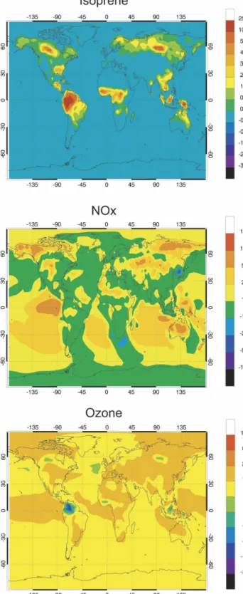
in the isoprene mixing ratio near the surface, when the isoprene emissions specified according to Guenther et al. (1995) are uniformly multiplied by 2. Enhancements of more than 1–2 ppbv are found in the isoprene mix-ing ratios in the forested areas of Canada, Alaska, Si-beria, Southeast Asia, and Australia. In the areas of tropical forests, the changes reach more than 4 ppbv and even more than 10 ppbv in the western part of the Amazon.
The relative changes in the NOx concentrations are shown in Fig. 13b. The percentage changes are very small in regions where the NOx concentrations are high, that is, in areas strongly influenced by fossil fuel and biomass burning emissions. Increases of the surface NOx concentrations of 40%–80% are predicted in Alaska, northern Canada, and Siberia, as well as in the central plains of the United States and in central Aus-tralia. In relative terms, significant increases are also found over the ocean, especially in the Southern Hemi-sphere, where the background NOx concentrations are very low, and where nitrogen oxides can be transported from the continent, particularly during winter. The re-sulting change in surface ozone is shown in Fig. 13c for July. As expected, the largest percentage increases in the ozone concentration are found where elevated val-ues of NOx are predicted. Climate-generated doubling in the isoprene and soil NOx emissions should lead to an increase in the surface ozone concentration by 5%– 10% in most areas during July, and even to up to 25% in specific areas (i.e., equatorial Pacific, central United States, Siberia, and sub-Sahara). A decrease in the sur-face ozone density by a few percent is predicted in the Amazon, due to the direct reaction of this biogenic hydrocarbon with ozone.
Finally, we assess the potential impact of climate-induced changes in the emissions associated with bio-mass burning. Here again, the future magnitude of these emissions is unknown. An intensification of wild-fires is often associated with heat waves in the extra-tropics. However, more frequent fires could also lead to the destruction of the forest with a progressive reduc-tion in fire frequency and intensity. Again, in order to quantify the sensitivity of potential changes in wildfire emissions, we consider a scenario (case H) in which biomass burning emissions in 2100 are assumed to be twice the emissions of the year 2000, while the other emissions and the change in climate are specified as in case E. The level of methane in 2100 is assumed to be 3.6 ppmv. Figure 14 shows the impact of the biomass burning doubling on surface ozone during July. The
FIG. 13. Impact of a uniform doubling in the emissions of iso-prene (vegetation) and nitric oxide (soils) for July conditions: (a) absolute change (ppbv) in the surface concentration of isoprene; (b) relative change (percent) in the surface concentration of NOx; and (c) relative change (percent) in the surface concentration of ozone (case G⫺ case E).
changes are most pronounced in the Tropics (10%– 15%) and in the summer boreal regions, specifically northern Canada, where large fires are assumed to oc-cur. As climate-driven changes in wildfire frequency are expected to be more pronounced at high latitudes than in the Tropics (Stocks et al. 1998; Flannigan et al. 2000; Amiro et al. 2001), it is likely that this climate-related effect will be most pronounced in the polar re-gions of the Northern Hemisphere.
6. Conclusions
Model calculations performed with the MOZART-2 model driven by the dynamics provided by the coupled ECHAM5/MPI-OM-1 atmosphere–ocean model show that substantial changes in the concentration of tropo-spheric ozone should have resulted from increasing emissions of chemical compounds in response to human activities. Since the preindustrial era, the surface con-centration of ozone should have nearly doubled in many parts of the world, with increases reaching a fac-tor of 3–4 in the industrialized regions of the Northern Hemisphere. Future changes in ozone will depend on several factors including population growth, economic development, and political decisions. Model predictions must therefore rely on scenarios. Most of these sce-narios suggest that the levels of air pollutants and spe-cifically of ozone will increase dramatically in South and Southeast Asia during the next decades. On the basis of the A2P scenario adopted in the present study, monthly averaged summertime surface ozone mixing ratios could reach 80 ppbv in these regions by the year 2100. Changes are expected to be smaller in the
indus-trialized regions of Europe and North America, where emissions are not expected to increase substantially.
The impact of future climate changes on the compo-sition of the troposphere is not well quantified because it depends on the evolution of a multitude of climate-related factors. Models show that the climate-driven increase in the tropospheric water vapor content, which should increase the concentrations of the OH and HO2
radicals, should somewhat damp the ozone increase ex-pected from enhanced emissions of ozone precursors such as NOx. Our model calculates a reduction in ozone of typically 5%–10% in the extratropics during sum-mertime in response to this climate-related effect. In the Tropics, however, ozone increases are amplified by 5%–8% (zonal mean) because of enhanced lightning activity predicted to occur in a warmer and wetter cli-mate. Changes can, however, be locally substantially larger in regions where meteorological flows are strongly modified as a result of a future climate change. The impact of the climate changes on ozone calculated for the A2P scenario is generally smaller than the un-certainty in future ozone associated with the unknown changes in future methane concentrations.
Table 4 provides the changes between 2000 and 2100 in the globally averaged ozone mixing ratio on different model levels (January and July conditions) in response to prescribed changes in the anthropogenic emissions of ozone precursors and to calculated climate changes in the twenty-first century. The changes derived for a case in which the two types of perturbations are combined are also provided. When comparing these results with, for example, those of Johnson et al. (1999), it appears that the changes associated with the prescribed human-induced emissions (A2P scenario) are typically a factor
FIG. 14. Impact of a geographically uniform doubling in biomass burning emissions on the surface concentration of ozone (July average) calculated for year 2100 conditions (A2P emission sce-nario; 2⫻CO2climate) (case H⫺ case E).
TABLE4. Globally averaged ozone mixing ratio (ppbv) on dif-ferent model surfaces as calculated for year 2000 conditions, and changes (ppbv) in year 2100 resulting from emissions of chemical compounds, climate change (A2P scenario), and combined effects.
Scenario 950 hPa 770 hPa 500 hPa 320 hPa January Baseline case (2000) 22.9 31.4 41.3 56.3 Effects of emissions ⫹12.4 ⫹16.9 ⫹22.3 ⫹23.9 Effects of climate change ⫺1.2 ⫺1.3 ⫹0.2 ⫹1.3 Combined effects ⫹10.5 ⫹14.3 ⫹20.5 ⫹23.2 July Baseline case (2000) 26.7 33.9 46.9 61.4 Effects of emissions ⫹14.8 ⫹18.7 ⫹24.8 ⫹28.1 Effects of climate change ⫺1.0 ⫺1.2 ⫹1.0 ⫹1.6 Combined effects ⫹12.6 ⫹16.0 ⫹24.7 ⫹28.6
of 2–3 larger in our study. One should remember, how-ever, that the adopted scenarios for these emissions are very different in the two model studies. The reduction in the ozone concentration resulting directly from cli-mate change is about a factor of 2 larger in the study of Johnson et al. (1999) than in the present model simu-lations. This is probably explained by the fact that, in the present study, the relatively large positive effect resulting from changes in lightning NOx production compensates to a certain extent the negative effect as-sociated with the calculated increase in the tropop-sheric water vapor abundance.
Besides the direct climate-related perturbations simulated by the general circulation model, other indi-rect effects could have a substantial effect on future ozone. These include changes in the temperature-dependent emissions of biogenic compounds, changes in the frequency and intensity of wildfires, changes in surface deposition processes associated with ecosystem perturbations, and changes in sea–air exchanges and in dust mobilization. Our model simulations show that a doubling in the biogenic isoprene and soil NO emis-sions, and in the biomass burning emissions should have a significant effect on surface ozone. Changes in weather patterns, which have not been considered ex-plicitly in the present study, could have a significant impact on future air quality, especially if the frequency of occurrence of summertime air stagnation events (a meteorological situation that favors the formation of ozone episodes in the extratropics) were to change in response to climate change (Mickley et al. 2004). Changes in the phase of the North Atlantic Oscillation could affect the long-range transport of pollutants from North America to Europe (Li et al. 2002). Increased ventilation from the boundary layer due to enhanced convection could also modify the surface concentration of pollutants (Rind et al. 2001). A further study will attempt to address these questions.
Acknowledgments. The authors thank Hauke
Schmidt for suggesting improvements on the manu-script and Ivar Isaksen for providing the model sce-narios on chemical emissions used in the present study. They also acknowledge the support provided by the MOZART team at the National Center for Atmo-spheric Research (NCAR). M. Saunois was supported by the Phytem Program of the Ecole Normale Supérieure (Cachan) and by the Pierre and Marie Curie University (Paris 6). This work was financed in part by the German BMBF under the COMMIT Project. The model simulations were performed on the NEC SX-6 supercomputer installed at the German Climate Com-puter Center (DKRZ) in Hamburg, Germany.
REFERENCES
Amiro, B. D., B. J. Stocks, M. E. Alexander, M. D. Flannigan, and B. M. Wotton, 2001: Fire, climate change, carbon and fuel management in the Canadian boreal forest. Int. J. Wildland Fire, 10, 405–413.
Anfossi, D., S. Sandroni, and S. Viarengo, 1991: Tropospheric ozone in the ninetenth century: The Moncalieri series. J. Geophys. Res., 96, 17 349–17 352.
Berntsen, T., I. S. A. Isaksen, J. S. Fuglestvedt, G. Myhre, T. A. Larsen, F. Stordal, R. S. Freckleton, and K. P. Shine, 1997: Effects of anthropogenic emissions on tropospheric ozone and its radiative forcing. J. Geophys. Res., 102, 21 239–21 280. ——, ——, G. Myhre, and F. Stordal, 2000: Time evolution of tropospheric ozone and its radiative forcing. J. Geophys. Res.,
105, 8915–8930.
Brasseur, G. P., J. T. Kiehl, J.-F. Müller, T. Schneider, C. Granier, X. Tie, and D. Hauglustaine, 1998: Past and future changes in global tropospheric ozone: Impact on radiative forcing. Geo-phys. Res. Lett., 25, 3807–3810.
Crutzen, P. J., 1988: Tropopsheric ozone: An overview. Tropo-spheric Ozone, I. S. A. Isaksen, Ed., Reidel, Dordrecht, 3–32. Dlugokencky, E. J., L. P. Steele, P. M. Lang, and K. A. Masarie, 1994: The growth rate and distribution of atmospheric meth-ane. J. Geophys. Res., 99, 17 021–17 043.
European Commission, 2003: Ozone-climate interactions. Air Pollution Res. Rep. 81, Directorate General for Research, Environment and Sustainable Development Programme, EUR 20623, 143 pp.
Fiore, A. M., D. J. Jacob, B. D. Field, D. G. Streets, S. D. Fernandes, and C. Jang, 2002: Linking ozone pollution to climate change: The case for controlling methane. Geophys. Res. Lett., 29, 1919, doi:10.1029/2002GL015601.
Flannigan, M. D., B. J. Stocks, and B. M. Wotton, 2000: Climate change and forest fires. Sci. Total Environ., 262, 221–229. Gauss, M., and Coauthors, 2003: Radiative forcing in the 21st
century due to ozone changes in the troposphere and the lower stratosphere. J. Geophys. Res., 108, 4292, doi:10.1029/ 2002JD002624.
GLOBALVIEW-CH4, 2001: Cooperative Atmospheric Data Inte-gration Project—Methane. NOAA/CMDL, Boulder, CO, CD-ROM. [Available online at ftp.cmdl.noaa.gov/ccg/ch4/ GLOBALVIEW.]
Grenfell, J. L., D. T. Shindell, and V. Grewe, 2003: Sensitivity studies of oxidative changes in the troposphere in 2100 using the GISS GCM. Atmos. Chem. Phys., 3, 1267–1283. Grewe, V., M. Dameris, R. Hein, R. Sausen, and B. Steil, 2001:
Future changes of the atmospheric composition and the im-pact of climate change. Tellus, 53B, 103–121.
——, ——, C. Fichter, and R. Sausen, 2002: Impact of aircraft NOx emissions. Part 1: Interactively coupled climate-chemistry simulations and sensitivities to climate-climate-chemistry feedback, lightning and model resolution. Meteor. Z., 11, 177–186.
Guenther, A., and Coauthors, 1995: A global model of natural volatile organic compound emissions. J. Geophys. Res., 100, 8873–8892.
Hack, J. J., 1994: Parameterization of moist convection in the Na-tional Center for Atmospheric Research Community Climate Model (CCM). J. Geophys. Res., 99, 5541–5568.
Hauglustaine, D. A., and G. P. Brasseur, 2001: Evolution of tro-pospheric ozone under anthropogenic activities and
associ-ated radiative forcing of climate. J. Geophys. Res., 106, 32 337–32 360.
Holtslag, A. A. M., and B. Boville, 1993: Local versus nonlocal boundary-layer diffusion in a global climate model. J. Cli-mate, 6, 1825–1842.
Horowitz, L., and Coauthors, 2003: A global simulation of tropo-spheric ozone and related tracers: Description and evaluation of MOZART, version 2. J. Geophys. Res., 108, 4784, doi:10.1029/2002JD002853.
Houghton, J. T., Y. Ding, D. J. Griggs, M. Noguer, P. J. van der Linden, X. Dai, K. Maskell, and C. A. Johnson, Eds., 2001: Climate Change 2001: The Scientific Basis. Cambridge Uni-versity Press, 881 pp.
Johnson, C. E., W. J. Collins, D. S. Stevenson, and R. G. Derwent, 1999: Relative roles of climate and emissions changes on fu-ture tropospheric oxidant concentrations. J. Geophys. Res.,
104, 18 631–18 645.
Lamarque, J.-F., P. Hess, L. Emmons, L. Buja, W. Washington, and C. Granier, 2005: Tropospheric ozone evolution between 1890 and 1990. J. Geophys. Res., 110, D08304, doi:10.1029/ 2004JD005537.
Lathière, J., D. A. Hauglustaine, N. De Noblet-Ducoudre, G. Krinner, and G. Folberth, 2005: Past and future changes in biogenic volatile organic compound emissions simulated with a global dynamic vegetation model. Geophys. Res. Lett., 32, L20818, doi:10.1029/2005GL024164.
Latif, M., and Coauthors, 2004: Reconstructing, monitoring, and predicting multidecadal-scale changes in the North Atlantic thermohaline circulation with sea surface temperature. J. Cli-mate, 17, 1605–1614.
Lelieveld, J., and R. van Dorland, 1995: Model simulations of ozone chemistry changes in the troposphere and consequent radiative forcing of climate during industrialization. Atmo-spheric Ozone As a Climate Gas, W. C. Wang and I. S. A. Isaksen, Eds., NATO ASI Series, Vol. 32, Springer-Verlag, 227–258.
Li, Q. B., and Coauthors, 2002: Transatlantic transport of pollu-tion and its effects on surface ozone in Europe and North America. J. Geophys. Res., 107, 4166, doi:10.1029/ 2001JD001422.
Lin, S. J., and R. B. Rood, 1996: Multidimensional flux-form semi-Lagrangian transport schemes. Mon. Wea. Rev., 124, 2046– 2070.
Marsland, S. J., H. Haak, J. H. Jungclaus, M. Latif, and F. Röske, 2003: The Max-Planck-Institute global ocean/sea ice model with orthogonal curvilinear coordinates. Ocean Modell., 5, 91–127.
Mickley, L. J., P. P. Murti, D. J. Jacob, J. A. Logan, D. Rind, and D. Koch, 1999: Radiative forcing from tropospheric ozone calculated with a unified chemistry-climate model. J. Geo-phys. Res., 104, 30 153–30 172.
——, D. J. Jacob, B. D. Field, and D. Rind, 2004: Effects of future climate change on regional air pollution episodes in the United States. Geophys. Res. Lett., 31, L24103, doi:10.1029/ 2004GL021216.
Murazaki, K., and P. Hess, 2006: How does climate change con-tribute to surface ozone change over the United States? J. Geophys. Res., 111, D05301, doi:10.1029/2005JD005873. Pavelin, E. G., C. E. Johnson, S. Rughooputh, and R. Toumi,
1999: Evaluation of pre-industrial surface ozone
measure-ments made using Schonbein’s method. Atmos. Environ., 33, 919–929.
Prather, M., and Coauthors, 2003: Fresh air in the 21st century? Geophys. Res. Lett., 30, 1100, doi:10.1029/2002GL016285. Price, C., and D. Rind, 1993: What determines the
cloud-to-ground lightning fraction in thunderstorms? Geophys. Res. Lett., 20, 463–466.
——, and ——, 1994: Possible implications of global climate change on global lightning distributions and frequencies. J. Geophys. Res., 99 (D5), 10 823–10 832.
Rasch, P. J., N. M. Mahowald, and B. E. Eaton, 1997: Represen-tations of transport, convection and the hydrologic cycle in chemical transport models: Implications for the modeling of short lived and soluble species. J. Geophys. Res., 102, 28 127– 28 138.
Rind, D., J. Lerner, and C. McLinden, 2001: Changes of tracer distribution in the doubled CO2 climate. J. Geophys. Res.,
106, 28 061–28 079.
Roeckner, E., and Coauthors, 2003: The atmospheric general cir-culation model ECHAM5. Part I: Model description. Rep. 349, Max Planck Institute for Meteorology, Hamburg, Ger-many, 349 pp.
——, and Coauthors, 2006: Sensitivity of simulated climate to horizontal and vertical resolution in the ECHAM5 atmo-sphere model. J. Climate, 19, 3771–3791.
Sanderson, M. G., C. D. Jones, W. J. Collins, C. E. Johnson, and R. G. Derwent, 2003: Effect of climate change on isoprene emissions and surface ozone levels. Geophys. Res. Lett., 30, 1936, doi:10.1029/2003GL017642.
Shallcross, D. E., and P. S. Monks, 2000: New directions: AQ role for isoprene in biosphere-climate-chemistry feedbacks. At-mos. Environ., 34, 1659–1660.
Shindell, D. T., G. A. Schmidt, R. L. Miller, and D. Rind, 2001: Northern Hemisphere winter climate response to greenhouse gas, ozone, solar, and volcanic forcing. J. Geophys. Res., 106, 7193–7210.
——, G. Faluvegi, and N. Bell, 2003: Pre-industrial-to-present-day radiative forcing by tropopsheric ozone from improved simu-lations with the GISS chemistry-climate GCM. Atmos. Chem. Phys., 3, 1675–1702.
Stevenson, D. S., C. E. Johnson, W. J. Collins, R. G. Derwent, K. P. Shine, and J. M. Edwards, 1998: Evolution of tropo-spheric ozone radiative forcing. Geophys. Res. Lett., 25, 3819– 3822.
——, ——, ——, ——, and J. M. Edwards, 2000: Future estimates of tropospheric ozone radiative forcing and methane turn-over—The impact of climate change. Geophys. Res. Lett., 27, 2073–2076.
——, R. Doherty, M. Sanderson, C. Johnson, B. Collins, and D. Derwent, 2005: Impacts of climate change and variability on tropopsheric ozone and its precursors. Faraday Discuss., 130, 1–17.
Stocks, B. J., and Coauthors, 1998: Climate change and forest fire potential in Russian and Canadian boreal forests. Climate Change, 38, 1–13.
Thompson, A. M., K. B. Hogan, and J. S. Hoffman, 1992: Meth-ane reductions—Implications for global warming and atmo-spheric chemical change. Atmos. Environ., 26A, 2665–2668. van Dorland, R., F. J. Dentener, and J. Lelieveld, 1997: Radiative
forcing due to tropospheric ozone and sulfate aerosols. J. Geophys. Res., 102, 28 079–28 100.
of ozone measurements made in the nineteenth century. Na-ture, 332, 240–242.
Wang, Y., and D. J. Jacob, 1998: Anthropogenic forcing on tro-pospheric O3and OH since preindustrial times. J. Geophys.
Res., 103, 10 757–10 768.
Yienger, J. J., and H. Levy II, 1995: Empirical model of global soil-biogenic NOx emissions. J. Geophys. Res., 100, 11 447– 11 464.
Zeng, G., and J. A. Pyle, 2003: Changes in tropospheric ozone between 2000 and 2100 modeled in a chemistry-climate model. Geophys. Res. Lett., 30, 1392, doi:10.1029/ 2002GL016708.
Zhang, G. J., and N. A. McFarlane, 1995: Sensitivity of climate simulations to the parameterization of cumulus convection in the Canadian Climate Centre general circulation model. At-mos.–Ocean, 33, 407–446.