The Minimized Power Geometric model: An analytical mixing model for calculating polyphase rock viscosities consistent with experimental data

HAL Id: insu-00994202

https://hal-insu.archives-ouvertes.fr/insu-00994202

Submitted on 21 May 2014

HAL is a multi-disciplinary open access

archive for the deposit and dissemination of

sci-entific research documents, whether they are

pub-lished or not. The documents may come from

teaching and research institutions in France or

abroad, or from public or private research centers.

L’archive ouverte pluridisciplinaire HAL, est

destinée au dépôt et à la diffusion de documents

scientifiques de niveau recherche, publiés ou non,

émanant des établissements d’enseignement et de

recherche français ou étrangers, des laboratoires

publics ou privés.

consistent with experimental data

Benjamin Huet, Philippe Yamato, Bernhard Grasemann

To cite this version:

Benjamin Huet, Philippe Yamato, Bernhard Grasemann. The Minimized Power Geometric model:

An analytical mixing model for calculating polyphase rock viscosities consistent with experimental

data. Journal of Geophysical Research, American Geophysical Union, 2014, 119 (4), pp.3897-3924.

�10.1002/2013JB010453�. �insu-00994202�

RESEARCH ARTICLE

10.1002/2013JB010453

Key Points:

• The MPG model predicts the viscos-ity of polyphase rocks having power law phases

• The MPG model provides a bet-ter fit with experimental data than existing models

• The MPG model offers good poten-tial in structural geology and numerical modeling Supporting Information: • Readme • Text S1 Correspondence to: B. Huet, benjamin.huet@univie.ac.at Citation:

Huet, B., P. Yamato, and B. Grasemann (2014), The Minimized Power Geometric model: An analytical mixing model for calculating polyphase rock viscosities consistent with experimen-tal data, J. Geophys. Res. Solid Earth, 119, doi:10.1002/2013JB010453.

Received 21 JUN 2013 Accepted 4 APR 2014

Accepted article online 9 APR 2014

The Minimized Power Geometric model: An analytical mixing

model for calculating polyphase rock viscosities consistent

with experimental data

B. Huet1_{, P. Yamato}2,3_{, and B. Grasemann}1

1_{Department of Geodynamics and Sedimentology, University of Vienna, Vienna, Austria,}2_{Géosciences Rennes, Université}

de Rennes 1 - UMR 6118, Rennes, France,3_{Géosciences Rennes, CNRS - UMR 6118, Rennes, France}

Abstract

Here we introduce the Minimized Power Geometric (MPG) model which predicts the viscosity of any polyphase rocks deformed during ductile flow. The volumetric fractions and power law parameters of the constituting phases are the only model inputs required. The model is based on a minimization of the mechanical power dissipated in the rock during deformation. In contrast to existing mixing models based on minimization, we use the Lagrange multipliers method and constraints of strain rate and stress geometric averaging. This allows us to determine analytical expressions for the polyphase rock viscosity, its power law parameters, and the partitioning of strain rate and stress between the phases. The power law bulk behavior is a consequence of our model and not an assumption. Comparison of model results with 15 published experimental data sets on two-phase aggregates shows that the MPG model reproduces accurately both experimental viscosities and creep parameters, even where large viscosity contrasts are present. In detail, the ratio between experimental and MPG-predicted viscosities averages 1.6. Deviations from the experimental values are likely to be due to microstructural processes (strain localization and coeval other deformation mechanisms) that are neglected by the model. Existing models that are not based on geometric averaging show a poorer fit with the experimental data. As long as the limitations of the mixing models are kept in mind, the MPG model offers great potential for applications in structural geology and numerical modeling.

1. Introduction

Lower crustal and upper mantle rocks are typically polyphase materials that deform in creep regimes. Their effective viscosities depend on temperature, strain rate, and anisotropy, as well as on composition (rheol-ogy and amounts of the constituting minerals). The mechanical control of the later factor is strong [Kirby, 1985]. The best natural examples of this interrelation are the ductile shear zones that show strain localiza-tion due to weakening by metamorphic reaclocaliza-tions [Pennacchioni, 1996; Furusho and Kanagawa, 1999; Handy

and Stünitz, 2002; Gueydan et al., 2003; Jolivet et al., 2005; Terry and Heidelbach, 2006; Hobbs et al., 2010; Oliot et al., 2010; Angiboust et al., 2011; Grasemann and Tschegg, 2012]. Quantifying the viscosity of polyphase

rocks and its changes with metamorphic reactions is therefore of crucial importance for understanding the strength of the lower crust and upper mantle. It is, though, still an open issue [Bürgmann and Dresen, 2008]. Several laboratory [Jordan, 1987; Tullis et al., 1991; Bloomfield and Covey-Crump, 1993; Bons and Urai, 1994;

Tullis and Wenk, 1994; Dresen et al., 1998; Bruhn et al., 1999; Ji et al., 2001; Jin et al., 2001; Xiao et al., 2002; Rybacki et al., 2003; Barnhoorn et al., 2005; Dimanov and Dresen, 2005] and numerical [Tullis et al., 1991; Treagus and Lan, 2000; Madi et al., 2005; Takeda and Griera, 2006; Groome et al., 2006; Jessell et al., 2009; Dabrowski et al., 2012] experiments on two-phase aggregates have already addressed this issue. They

char-acterized the way the bulk viscosity of a few aggregates changes with their composition. These studies also improved our understanding of the processes occurring in polyphase rocks during deformation. How-ever, unlike the diversity of natural rocks, the number of experiments is limited. An accurate experimental description of all the polyphase rocks is, therefore, not available.

Theoretically, mixing models can be used to estimate the viscosity of any polyphase rock if the amounts and the mechanical behaviors of its constituting minerals are known. Such models can be classified into three families: (1) phenomenological models [Voigt, 1928; Reuss, 1929; Tullis et al., 1991; Ji and Zhao, 1993;

[Hutchinson, 1976; Zhou, 1995; Jiang et al., 2005], and (3) models derived with the self-consistent approach [Budiansky, 1965; Hill, 1965; Duva, 1984; Yoon and Chen, 1990; Treagus, 2002; Jiang, 2013].

Applying these models to lower crustal and mantle rocks is, however, not straightforward. They are indeed either designed only for two-phase materials [Budiansky, 1965; Hill, 1965; Duva, 1984; Yoon and Chen, 1990;

Tullis et al., 1991; Handy, 1994a, 1994b; Treagus, 2002], depend on approximately constrained empirical

parameters [Ji and Zhao, 1993; Ji et al., 2003; Ji, 2004], provide viscosity bounds [Voigt, 1928; Reuss, 1929;

Hutchinson, 1976; Zhou, 1995; Jiang et al., 2005], or require an iteration process [Ji and Zhao, 1993; Zhou,

1995; Ji et al., 2003; Jiang et al., 2005].

In this paper, we present a new mixing model based on constrained minimization of the mechanical power: the Minimized Power Geometric model (MPG model). This minimization is, for the first time, carried out analytically with the Lagrange multipliers method. We thus provide a fast and precise way to estimate the bulk viscosity of any polyphase rock, as well as its bulk creep parameters and the strain rate and stress in its constituting phases.

The method and the derivation of the MPG model are presented first. The results are then analyzed, and the estimates of the MPG model are compared with existing laboratory and numerical experiments. Our model is also compared with existing mixing models in order to assess the ability of all these models to reproduce the experimental data sets. The limitations and the advantages of our model are finally discussed.

2. Theory and Method of Calculation

This section, which presents the theory and the method used to develop the new mixing model, formalizes and extends a method introduced in geology by Handy [1990]. Materials considered here are assumed to have isotropic properties and incompressible behaviors that do not depend on pressure. The derivations are carried out with the second invariants of the deviatoric strain rate and stress tensors, e and s, which are hereafter simply called strain rate and stress. The notations used in the paper are presented in the Notation.

2.1. Mechanical Power Dissipated in a Power Law Material

In a viscous material, the viscosity𝜂 relates strain rate e to stress s:

s = 2𝜂e. (1)

Laboratory experiments suggest that the steady state behavior of creeping minerals and rocks can be described by a power law equation:

e = Asnexp(−Q

RT

)

, (2)

where n, Q, A, R, and T stand respectively for the stress exponent, activation energy, preexponential factor, gas constant, and absolute temperature [Kohlstedt et al., 1995]. The creep parameters n, Q, and A are mate-rial factors, and A can include the effect of average grain size as well as the water and oxygen fugacities. To simplify the following derivations, a condensed form of the power law equation is adopted:

e = Bsn_{, (3)} where B = A exp(−Q RT ) . (4)

Combining equations (1) and (3), the behavior of a homogeneous power law material can thus be described by an effective viscosity that depends on either strain rate or stress:

𝜂 =e(1−n)∕n

2B1∕n =

s1−n

2B. (5)

Viscous creep is accompanied by dissipation of mechanical power [Ranalli, 1995]:

P = 2𝜂e2₌ s2

2𝜂, (6)

The mechanical power dissipated in a homogeneous power law material is then given by substituting equation (5) into equation (6):

P =e

(n+1)∕n

B1∕n = Bs

2.2. Mechanical Power Dissipated in a Polyphase Rock

A polyphase rock is an aggregate of N different phases i with volumetric fractions𝜙i(the fractions sum up

to 1). Each phase corresponds to all grains of a mineral. For example, the phases constituting granite are quartz, mica, plagioclase, and alkaline feldspar. In that particular case, N = 4.

In the following, we make three assumptions:

1. The distribution of the different phases constituting the aggregate is homogeneous and isotropic, and these phases do not present any shape- or crystallographic-preferred orientation. This allows us to consider constant𝜙isets and to avoid theoretical problems related to anisotropic viscosity.

2. The only deformation mechanism is incompressible viscous creep of each phase i, described by a power law with known parameters ni, Aiand Qi. Even if elastic deformation must be present, the contribution of

elastic strain rate close to steady state is considered to be negligible. 3. All the grains from the same phase i have the same strain rate eiand stress si.

These assumptions have been used more or less implicitly for developing previous mixing models [Handy, 1990; Tullis et al., 1991; Handy, 1994a, 1994b; Ji, 2004; Ji and Zhao, 1993; Ji et al., 2003; Jiang et al., 2005;

Zhou, 1995]. They are also crucial for the development of our model. It must, however, be noted that the

third assumption is very strong because it leads locally to a contradiction with the equations of stress and strain rate continuity. While ensuring continuity between the grains belonging to the same phase, it does not respect this principle at the boundary between grains belonging to different phases. The validity and consequences of these conditions are extensively discussed in section 7.

The bulk viscosity of a polyphase rock̄𝜂 can be calculated in the same way as for homogeneous material, as the ratio of the bulk stress̄s over the bulk strain rate ̄e:

̄𝜂 = ̄s

2̄e. (8)

On the one hand, the bulk mechanical power can be expressed with this bulk viscosity according to equation (6):

̄P = 2̄𝜂̄e2₌ ̄s2

2̄𝜂. (9)

On the other hand, assumption 2 allows us to calculate the mechanical power dissipated in a polyphase rock by summing the mechanical power dissipated in each phase P_iweighted by the phase fraction𝜙_i[Handy, 1990] such that

̄P =∑

i

𝜙iPi. (10)

Throughout the paper, sums and products are calculated over the N phases when no lower and upper bounds are specified. Using assumptions 2 and 3, equations (7) and (10) can be combined to express ̄P as a function of phase strain rates or stresses:

̄P =∑ i 𝜙iB −1∕ni i e (ni+1)∕ni i = ∑ i 𝜙iBis ni+1 i . (11)

In equation (11), the sets of e_iand s_iare unknown. Here we calculate the e_iand s_ithat minimize the mechan-ical power dissipated in the polyphase rock. Minimizing the power dissipated in a polyphase aggregate for calculating a bulk viscosity has been proposed for the first time by Handy [1994a, 1994b] and applied in the studies of Zhou [1995] and Jiang et al. [2005]. This amounts to using the principle of least action that is commonly used in elastic polycrystals studies (see the review by Markov [1999]). It must be emphasized that the principle of least action has been developed for transition between equilibrium states with conser-vation of energy and that its application to nonequilibrium process leads to steady state if the relationship between the driving force (the stress) and the flux (the strain rate) is linear [de Groot and Mazur, 1984]. It is then possible to estimate the bulk viscositȳ𝜂 as follows: once the set of ei(resp. si) that minimizes ̄P is

determined for a given bulk strain ratēe (resp. stress ̄s), the mechanical power is calculated with equation (11) and the effective viscosity of the aggregate is calculated with equation (9).

2.3. Which Constraint for the Minimization?

The absolute minimum of the mechanical power is zero. This value implies that the phases of a deformed polyphase rock do not deform. As this is in contradiction to assumption 2, an additional relation between the phase and bulk strain rates (resp. stresses) is therefore required. Such a relation has to describe the strain rate (or stress) partitioning between the phases for a given bulk strain rate (resp. stress). This will be used as a constraint for the minimization. Different types of constraints can be considered.

2.3.1. Homogeneity Constraints

Homogeneous strain rate (ei=̄e, 1 ≤ i ≤ N) and homogeneous stress (si=̄s, 1 ≤ i ≤ N) only apply to layered

media loaded along specific directions [Markov, 1999], which correspond to a limited number of cases. In these cases, the mechanical power cannot be minimized because the eior the siare fixed. The homogeneity

constraints are therefore not consistent with minimization of the power. They are also unrealistic for most rocks [Tullis et al., 1991].

2.3.2. Arithmetic Mean Constraints

A simple equation describes the strain rate partitioning in a layered material loaded perpendicular to its layering. The bulk strain rate is the arithmetic mean of the phase strain rates:

∑

i

𝜙iei−̄e = 0. (12)

Similarly, loading of a layered material parallel to its layering leads to a simple expression for the stress partitioning. The bulk stress is the arithmetic mean of the phase stresses:

∑

i

𝜙isi−̄s = 0. (13)

These two types of partitioning, which are in theory only valid for layered materials, have been used as constraints for minimizing the dissipated power in isotropic materials [Zhou, 1995].

A constraint derived from equation (12) has subsequently been proposed for taking into account strain dis-tribution at grain size scale [Jiang et al., 2005]. Since the deformation of minor weak phases is controlled by the stronger phase skeleton, they cannot experience an excessively large strain rate and their strain rates can be approximated by the bulk strain rate. This amounts to setting eitōe for the minor weak phases in

equation (12), and the corresponding derivation can therefore be adapted from the one using equation (12).

2.3.3. Geometric Mean Constraints

Following the use of the arithmetic mean of the phase strain rate or stress by Zhou [1995], we here use geo-metric mean constraints. These are derived from the previous constraints by simply replacing the arithmetic mean with the geometric mean. The geometric mean of strain rate is expressed by

∏

i

e𝜙i

i −̄e = 0 (14)

and the geometric mean of stress is expressed by ∏

i

s𝜙i

i −̄s = 0. (15)

There are two reasons to consider geometric averaging as a constraint. The first one is based on a theoretical argument [Aleksandrov and Aizenberg, 1966; Matthies and Humbert, 1993] that states that a function f which allows to average a physical property x

̄x = f−1 ( ∑ i 𝜙if (xi) ) , (16)

and its inverse property y = x−1

̄y = f−1 ( ∑ i 𝜙if (yi) ) , (17) so that ̄x = x−1−1_{, (18)}

provides an improvement in comparison to the arithmetic and harmonic means. The geometric mean fulfills this condition. The second reason is empirical and comes from the fact that mixing models based on the geometric mean provide a good fit with experimental data (see section 6 below).

The constraints (14) and (15) are used below to develop the MPG model. The arithmetic mean constraints having already been considered together with a numerical approach [Zhou, 1995], they are used here to develop an analytical version of the mixing models of Zhou [1995], to which the MPG model will be later compared (see sections 4 and 6.2).

2.4. The Lagrange Multipliers Approach

Previous studies used numerical iterations for minimizing the dissipated mechanical power [Zhou, 1995;

Jiang et al., 2005]. Here we use the Lagrange multipliers method [e.g., Stewart, 2002] outlined here. A

supplementary function L is defined by the mechanical power and the constraint C:

L = ̄P −𝜆C, (19)

where ̄P is given by equation (11),𝜆 is the Lagrange multiplier, and C is the chosen constraint given by equations (12), (13), (14), or (15). The constrained minimum of the mechanical power is found by setting simultaneously the N + 1 partial derivatives of L (N phase strain rates or stresses and one Lagrange multi-plier) to zero. Since the stress exponent in power laws is larger or equal to 1, ̄P is convex up. The value found with the Lagrange multiplier method is therefore a unique minimum.

3. Theoretical Determination of the Mixing Models

For each of the four constraints described in sections 2.3.2 and 2.3.3, one mixing model can be determined. These four models are referred to as Minimized Power Geometric/Arithmetic strain rate/stress models (MPGe, MPGs, MPAe, and MPAs models). Geometric or Arithmetic describes the type of mean used in the constraint, and strain rate or stress describes the quantity used in the constraint. In this section, we detail the determination of the MPGe model. The determination of the three other models follows the same steps and is presented in the supporting information. As section 3 mainly contains the derivations, the reader who is not interested can turn directly to section 4 where the results of theses calculations are provided.

The supplementary function is built by inserting equation (11) and constraint (14) into equation (19):

L(…, e_i, … , 𝜆)=∑ i 𝜙iB −1∕ni i e (ni+1)∕ni i −𝜆 ( ∏ i e𝜙i i −̄e ) . (20)

Setting all the partial derivatives of L to zero leads to a system of N equations:

𝜙iB −1∕ni i ni+ 1 ni e1∕ni i =𝜙i𝜆e 𝜙i−1 i ∏ j≠i e𝜙j j , 1 ≤ i ≤ N, (21) together with ∏ i e𝜙i i =̄e. (22)

3.1. Determination of the Strain Rate Partitioning

One phase i is considered (1≤ i ≤ N). Equation (21) is first simplified by isolating e1∕ni

i in the left-hand side:

e1∕ni i = B 1∕ni i n_i ni+ 1 𝜆e𝜙i−1 i ∏ j≠i e𝜙j j . (23)

Equation (23) is then multiplied by e_i:

e(ni+1)∕ni i = B 1∕ni i ni n_i+ 1𝜆e 𝜙i i ∏ j≠i e𝜙j j , = B1∕ni i n_i ni+ 1 𝜆∏ i e𝜙i i . (24)

and simplified with equation (22):

e(ni+1)∕ni i = B 1∕ni i ni n_i+ 1𝜆̄e. (25)

We then introduce the N effective viscosities of the phases calculated for homogeneous strain rate, as in equation (5): 𝜂i= ̄e (1−ni)∕ni 2B1∕ni i , (26)

which gives an expression for the Bi:

B_i= [ ̄e(1−ni)∕ni 2𝜂i ]ni . (27)

The introduction of this notation does not imply that homogeneous strain rate is assumed. Equation (27) is inserted into equation (25):

e(ni+1)∕ni i = n_i 2(ni+ 1) 𝜆 𝜂i ̄ēe(1−ni)∕ni, = ni 2(ni+ 1) 𝜆 𝜂īe ̄e(ni+1)∕ni. ₍₂₈₎

We also introduce a scaled Lagrange multiplier𝜉:

𝜉 = 𝜆_̄e. (29)

A relation between the N phase strain rates and the bulk strain rate is then found by setting equation (28) to the power n_i∕(n_i+ 1) and using the definition of the scaled Lagrange multiplier:

ei=̄e ( ni 2(ni+ 1) 𝜉 𝜂i )ni∕(ni+1) . (30)

Hence, these N equations give the value of the strain rate in each phase of the aggregate.

3.2. Determination of the Scaled Lagrange Multiplier𝝃

The e_iare eliminated from equation (22) by introducing the N equations (30):

̄e =∏ i ̄e𝜙i ( ni 2(ni+ 1) 𝜉 𝜂i )𝜙ini∕(ni+1) , =̄e ( 𝜉 2 )∑ i𝜙ini∕(ni+1)∏ i ( ni 𝜂i(ni+ 1) )𝜙ini∕(ni+1) . (31)

A new set of parameters is introduced:

a_i=∏

j≠i

(n_j+ 1). (32)

The powers in equation (31) are then simplified with

𝜙ini n_i+ 1= 𝜙iaini ∏ j(nj+ 1) (33) and ∑ i 𝜙ini n_i+ 1 = ∑ i𝜙iaini ∏ i(ni+ 1) . (34)

Equation (31) then becomes

̄e = ̄e ( 𝜉 2 )∑ i𝜙iaini∕∏i(ni+1)∏ i ( _n i 𝜂i(ni+ 1) )𝜙iaini∕∏j(nj+1) (35) and the value of the scaled Lagrange multiplier is

𝜉 = 2∏ i ( 𝜂i ni+ 1 ni )𝜙iaini∕∑j𝜙jajnj . (36)

3.3. Determination of the Bulk Viscosity

The minimum value of the mechanical power is calculated by inserting successively equations (30), (27), and (36) into equation (11): ̄P =∑ i 𝜙iB −1∕ni i e (ni+1)∕ni i , =∑ i 𝜙i2𝜂īe(ni−1)∕ni n_i 2(ni+ 1) 𝜉 𝜂i ̄e(ni+1)∕ni, = 2̄e2∏ i ( 𝜂i n_i+ 1 ni )𝜙iaini∕ ∑ i𝜙jajnj∑ i 𝜙ini ni+ 1 . (37)

Combining equations (9) and (37) gives the value of the bulk viscosity for the MPGe model:

̄𝜂 =∑ i 𝜙ini ni+ 1 ∏ i ( 𝜂i n_i+ 1 ni )𝜙iaini∕∑i𝜙jajnj . (38)

3.4. Determination of the Bulk Creep Parameters

The strain rate and temperature dependency of the bulk viscosity are explicitly stated by introducing equations (4) and (26) in equation (38):

̄𝜂 =∑ i 𝜙ini ni+ 1 ×∏ i ( ̄e(1−ni)∕ni 2A1∕ni i exp ( Qi niRT ) ni+ 1 ni )𝜙iaini∕ ∑ i𝜙jajnj . (39)

This equation can be simplified into a product of three terms:

̄𝜂 =[̄e∑i𝜙iai(1−ni)∕ ∑ i𝜙iaini]_× [ exp ( 1 RT ∑ i𝜙iaiQi ∑ i𝜙iaini )] × ⎡ ⎢ ⎢ ⎣ ∑ i 𝜙ini ni+ 1 ∏ i ( n_i+ 1 2A1∕ni i ni )𝜙iaini∕∑i𝜙jajnj⎤ ⎥ ⎥ ⎦. (40)

If the bulk behavior obeyed a power law, the bulk effective viscosity could be calculated with equation (5):

̄𝜂 =[̄e(1−̄n)∕̄n] [_exp( ̄Q ̄nRT )] [ 1 2 ̄A1∕̄n ] , (41)

wherēn, ̄Q, and ̄A would be the bulk creep parameters.

In equations (40) and (41), the bulk viscosity is split into three factors: a factor with a power of the bulk strain rate, an Arrhenius-type factor depending on temperature, and a factor containing only material parameters. The power of the bulk strain rate that appears in the first factor of equation (40) is treated first:

∑ i𝜙iai(1 − ni) ∑ i𝜙iaini = 1 − ∑ i𝜙iaini ∑ i𝜙iai ∑ i𝜙iaini ∑ i𝜙iai . (42)

The first factors of equations (40) and (41) match exactly for

̄n = ∑ i𝜙iaini ∑ i𝜙iai . (43)

Using the definition of the bulk stress exponent that has just been determined, the second factors match for

̄Q =∑i𝜙iaiQi

∑

i𝜙iai

. (44)

The bulk preexponential factor is calculated by identifying the third factors of equations (40) and (41): 1 2 ̄A1∕̄n = ∑ i 𝜙ini ni+ 1 ∏ i ( n_i+ 1 2A1∕ni i ni )𝜙iaini∕∑i𝜙jajnj . (45)

Introducing the value of the bulk stress exponent, given by equation (43), into equation (45) leads to

̄A =⎛⎜ ⎜ ⎝ 1 2∑_i 𝜙ini ni+1 ⎞ ⎟ ⎟ ⎠ ̄n ∏ i ( 2A1∕ni i ni n_i+ 1 )̄n𝜙iaini∕∑i𝜙jajnj . (46)

Table 1. Bulk Viscosity, Phase Strain Rates or Phase Stresses, and Scaled Lagrange Multiplier for the Four Mixing Models

Phase Strain Ratese_i

Mixing Model Bulk Viscosity_̄𝜂a _{or Phase Stressess}

i Scaled Lagrange Multiplier𝜉b

MPGe ∑_i 𝜙ini ni+1 ∏ i ( 𝜂i ni+1 ni )_∑𝜙iaini i 𝜙j aj nj _̄e( ni 2(ni+1) 𝜉 𝜂i ) ni ni+1 ₂∏ i ( 𝜂i ni+1 ni )_∑𝜙iaini i 𝜙j aj nj MPGs _∑1 i_ni+1𝜙i ∏ i ( 𝜂i_ni1₊₁ )_∑𝜙iai i 𝜙j aj ̄s( 2 ni+1 𝜂i 𝜉 ) 1 ni+1 ₂∏ i ( 𝜂i_ni1₊₁ )_∑𝜙iai i 𝜙j aj MPAe ∑_i𝜙i𝜂i( ni 2(ni+1) 𝜉 𝜂i )ni+1 ̄e( ni 2(ni+1) 𝜉 𝜂i )ni ∑ i𝜙i ( _n i 2(ni+1) 𝜉 𝜂i )ni = 1 MPAs ⎛ ⎜ ⎜ ⎝ ∑ i𝜙_𝜂ii ( 2 n_i+ 1 𝜂i 𝜉 )ni+1 ni ⎞_⎟ ⎟ ⎠ −1 ̄s( 2 ni+1 𝜂i 𝜉 )1 ni ∑ i𝜙i ( ₂ ni+1 𝜂i 𝜉 )1 ni _{= 1}

a_{For the MPGe and MPAe models, 𝜂}

i=̄e(1−ni)∕ni∕2B

1∕ni

i . For the MPGs and MPAs models,

𝜂i=̄s1−ni∕2Bi;ai=∏j≠i(nj+ 1).

b_{The scaled Lagrange multiplier is the solution of a nonlinear equation for the two MPA models.}

Further simplification give the value of the bulk preexponential factor:

̄A = ( ∑ i 𝜙ini ni+ 1 )−̄n ∏ i ( ni ni+ 1 )𝜙iaini∕ ∑ i𝜙jaj∏ i A𝜙iai∕ ∑ i𝜙jaj i . (47)

Bulk creep parameters that correspond to a power law and that do not depend on temperature and on bulk strain rate can be determined for the MPGe model. Thus, if the phases follow a power law behavior, the bulk behavior defined by the MPGe model is also a power law behavior.

4. Analysis of the Mixing Models

The four mixing models determined in both section 3 (for the MPGe model) and supporting information (for the MPGs, MPAe, and MPAs models) are analyzed here. This section demonstrates the predictions of the four models for an anorthite-diopside aggregate in the wet dislocation creep regime. This example has been chosen because of the large difference in creep parameters and viscosity between anorthite (the weak phase) and diopside (the strong phase).

4.1. The Equations Defining the Mixing Models

The equations defining the four mixing models are summarized in Table 1. The two MPG models are fully analytical while the two MPA models are semianalytical. Their scaled Lagrange multipliers are calculated numerically by solving a nonlinear equation. The solution of this equation is then used for calculating the bulk viscosity and the strain rate or the stress in the phases.

For the four models, the bulk viscosity appears as a weighted mean of the phase viscosities calculated for homogeneous strain rate or stress. The type of mean in these equations depends on the constraint: geomet-ric mean for the MPG models, arithmetic mean for the MPAe model, and harmonic mean for the MPAs model. The weights are combinations of volumetric fractions, stress exponents, viscosities, and scaled Lagrange multiplier. Similar combinations appear in the expressions of the phase strain rates and stresses.

The equations in Table 1 are intricate because the stress exponents of the phases are different. They simplify for a homogeneous stress exponent. This simple case corresponds to a rock in which all the phases deform by diffusion creep (n = 1). It is also an approximation for a rock in which the phases deform by dislocation creep with stress exponents close to 3. In such cases, both MPG models predict the same bulk viscosity:

̄𝜂 =∏

i

𝜂𝜙i

i , (48)

which is exactly the geometric mean of the viscosities of the phases calculated for a homogeneous strain rate or a homogeneous stress. The scaled Lagrange multiplier of the MPA models can be calculated ana-lytically for homogeneous stress exponents. The bulk viscosity defined by the MPAe model is given by the

generalized mean of the phase viscosities calculated for homogeneous strain rate, with an exponent equal to −n:

̄𝜂 =(∑𝜙i𝜂i−n

)−1∕n

. (49)

For the MPAs model, the bulk viscosity is given by the generalized mean of the phase viscosities calculated for homogeneous stress, with an exponent equal to 1∕n:

̄𝜂 =(∑𝜙i𝜂

1∕n

i

)n

. (50)

Equations (49) and (50) simplify to a harmonic and arithmetic mean, respectively, for a polyphase rock containing phases deforming by diffusion creep.

4.2. The Bulk Viscosity

Figure 1a presents the bulk viscosity of an anorthite-diopside aggregate as a function of its diopside frac-tion. The predictions of the four mixing models are plotted together. The mixing models show three similar characteristics. The viscosity calculated for the two end-member compositions is similar to the end-member viscosity. The viscosity increases while the fraction of diopside increases. The models constrained by stress partitioning predict larger bulk viscosities than those constrained by strain rate partitioning. The first two characteristics are expected for any mixing model.

There are, however, major differences between the MPG models and the MPA models. The viscosity curves calculated with the MPG models have a smooth slope and are almost undistinguishable. The two MPG mod-els therefore predict bulk viscosities which are very similar. The trend of the curves on Figure 1a is close to linear. Since the y axis uses a logarithmic scale, this means that the bulk viscosity is close to the one calculated with a simple geometric mean. The viscosity curves calculated with the MPA models are in con-trast significantly different from each other (by several orders of magnitude), and the estimates of the MPA models bound those of the MPG models. The MPAe model leads to the lowest calculated viscosities with a convex down curve. The predicted bulk viscosity is close to the viscosity of anorthite when the aggregate contains less than 80% of diopside. It steepens up dramatically for larger diopside fractions. The evolution of the viscosity curve predicted by the MPAs model shows an opposite behavior.

4.3. The Partitioning of Strain Rate and Stress

The strain rate and stress in anorthite and diopside are presented as functions of the diopside fraction (Figures 1b and 1c). These curves characterize the partitioning of strain rate and stress predicted by the four mixing models. Both strain rates and stresses are normalized on the bulk values.

The evolutions of the curves predicted by the four mixing models are similar. For a given aggregate com-position, the strain rate in anorthite is larger than the bulk strain rate, and the stress is lower than the bulk stress. Further, the normalized strain rate increases, and the normalized stress decreases while the fraction of anorthite decreases. For anorthite fractions tending to zero, the limit value of its strain rate and stress is finite. The evolution of strain rate and stress in diopside is similar. The strain rate curves are translated at values lower than the bulk one, and the stress curves are translated at values larger than the bulk ones. This evolution implies that both the weak and the strong phases deform at higher strain rates while the aggregate gets richer in the strong phase and hence stronger.

However, the way that partitioning is quantified is model dependent. The evolution predicted by the two MPG models is characterized by a fairly constant slope, and both models predict almost identical parti-tioning. In contrast, the MPAe model predicts a dramatic increase of the phase strain rates (5 orders of magnitude for anorthite and 12 orders of magnitude for diopside) and an almost homogeneous stress close to the bulk value. In contrast, the MPAs model predicts a dramatic increase of the phase stresses and an almost homogeneous strain rate close to the bulk value. The MPA models therefore behave almost like models based on homogeneous strain rate or stress, such behaviors being generally unrealistic [Tullis et al., 1991].

4.4. The Bulk Creep Parameters

The bulk creep parameters of the MPG models determined in section 3 and supporting information are presented in Table 2. They only depend on the phase creep parameters and fractions and do not vary with temperature, strain rate, or stress. Thus, an aggregate of power law phases defined by the MPG models also

Figure 1. Mechanical behavior of anorthite-diopside aggregates as a function of the diopside fraction predicted by the MPGe(black solid curves), the MPGs(grey solid curves), the MPAe(black dotted curves), and the MPAs(grey dotted curves) models. (a) Bulk viscosity. (b) Normalized strain rate in the phases (an: anorthite, weak phase, di: diopside, strong phase). (c) Normalized stress in the phases. (d) Bulk stress exponent. (e) Bulk activation energy. (f ) Bulk preexponential factor. The phase strain rates and the stresses are normalized on the bulk values. Predictions are calculated for tem-perature of 1023 K and strain rate of 10−16_s−1_{. The bulk creep parameters are also calculated at other conditions in} order to show that the bulk creep parameters predicted by the MPA models depend on temperature and strain rate. The creep parameters of anorthite and diopside correspond to the dislocation creep regime in wet conditions [Dimanov and

Dresen, 2005].

follows a power law. The transmission of this behavior from the phases to the aggregate is not an assump-tion of the MPG models. Such a transmission has also been recognized in phenomenological mixing models based on geometric averaging [Tullis et al., 1991; Ji and Zhao, 1993; Ji et al., 2003] and is consequence of the geometric mean used in the constraints. Essentially speaking, multiplying strain rates, stress, or viscosities together allows the powers in the phases power laws to be regrouped together, leading to a bulk power law. The two MPG models give the same bulk stress exponent̄n and the same bulk activation energy ̄Q (Table 2). These bulk parameters are calculated as the arithmetic mean of the phase parameters weighted by𝜙_ia_i. For homogeneous phase stress exponents, the bulk stress exponent simplifies to the phase stress expo-nents, and the bulk activation energy simplifies to the arithmetic mean of the values of the separate phases

Table 2. Bulk Creep Parameters Calculated for the Minimized Power Geometric Models

Mixing Bulk Stress Bulk Activation Bulk Preexponential Model Exponent̄na _EnergȳQa _Factor̄Aa MPGe ∑_i𝜙ia_in_i∕ ∑_i𝜙iai ∑i𝜙iaiQi∕ ∑i𝜙iai ∏iA 𝜙iai∕ ∑ i𝜙jaj i × (∑ i 𝜙ini ni+1 )−̄n∏ i ( _n i ni+1 )𝜙iaini∕∑i𝜙jaj MPGs ∑_i𝜙iaini∕ ∑i𝜙iai ∑i𝜙iaiQi∕ ∑i𝜙iai ∏iA 𝜙iai∕∑i𝜙jaj i × ∑ i 𝜙i ni+1 ∏ i(ni+ 1)𝜙iai∕ ∑ i𝜙jaj Homogeneousn_ib _n i ∑i𝜙iQi ∏iA𝜙ii a_a i=∏j≠i(nj+ 1).

b_{For homogeneous stress exponent, both MPGeand MPGsmodels provide the same bulk creep parameters.}

(Table 2). As expected from their expressions, the evolution of ̄n and ̄Q with increasing diopside fraction shows a regular and close to linear increase from the anorthite value to the diopside value (Figures 1d and 1e).

The bulk preexponential factor ̄A of the MPGe and MPGs models are different (Table 2). The ratio between these expressions lies between 0.25 and 1 (see Appendix A). This implies that the value of ̄A corresponding to the MPGe model is larger than the one corresponding to the MPGs model (Figure 1f ). This also implies that the bulk viscosity predicted by the MPGe model is always lower than the bulk viscosity predicted by the MPGs model, as observed on Figure 1a. However, the bulk viscosity predicted by the two MPG models falls within the same order of magnitude. For homogeneous stress exponents, both MPG models predict the same bulk preexponential factor: the geometric mean of the phase preexponential factors (Table 2). In spite of the complexity of the expression which define it, the predicted bulk preexponential factor of anorthite-diopside aggregates decreases regularly when the diopside fraction increases (Figure 1f ). In contrast, the bulk creep parameters that correspond to the MPA models cannot be calculated analytically (see supporting information). Figures 1d–1f show the evolution of these parameters, calculated numerically for anorthite-diopside aggregates at different conditions of temperature and strain rate. The values of̄n,

̄Q, and ̄A predicted by the MPA models depend on temperature and on strain rate. Thus, even if the phases

have a power law behavior, this characteristic is not transmitted to the bulk behavior described by the MPA models.

5. Comparison With Experiments

The MPGe and MPGs models predict values of the bulk preexponential factor that are almost similar. This is the only difference between these two models, and it is the reason they predict similar bulk viscosities and partitioning. Below, these two models are thus referred to as a single MPG model, and only the predictions of the MPGe model are shown.

In this section, the predictions of the MPG model are compared with the published results of 15 experimen-tal data sets on two-phase materials. The predictions of the MPG model are calculated with the experimenexperimen-tal end-member viscosities and stress exponents using equation (38). When bulk creep parameters have been determined experimentally for the aggregates of intermediate compositions, bulk creep parameters are also calculated using equations (43), (44), and (47). Experiments which have been shown by Ji [2004] not to fall within the theoretical bounds are not considered here. In the following figures, the experimental data together with their errors (when reported) are represented by open symbols, and the predictions are represented by solid curves.

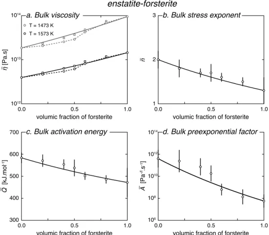
5.1. Enstatite-Forsterite Aggregates

In the experiments carried out by Ji et al. [2001], forsterite is stronger than enstatite, with a viscosity con-trast lower than 1 order of magnitude (Figure 2a). The same deformation mechanisms were observed in the phases deformed alone and in the two-phase aggregates. Since the deformation mechanisms do not change, it is legitimate to calculate the bulk viscosity of the aggregates using the end-member values. The evolution of the viscosity with increasing forsterite fraction shows a trend close to logarithmic (Figure 2a). This evolution is complicated by an S-shape trend which has been interpreted as the effect of

microstruc-Figure 2. (a–d) Bulk viscosity and bulk creep parameters of enstatite-forsterite aggregates as a function of the forsterite fraction: comparison between the experimental data set of Ji et al. [2001] (open circles) and the MPG model (solid curves). The experimental S-shape trend is highlighted with a dotted line. Viscosity values corrected for the porosity [Ji, 2004] are also shown (open squares). The vertical bars correspond to the fitting errors calculated during the regression of the creep parameters. Bulk strain rate: 10−6_s−1_{, temperature: 1473–1573 K, confining pressure: 0.1 MPa.}

tural changes [Ji et al., 2001]. For low forsterite fractions (lower than 0.4), the structure is weak-phase supported, whereas for large forsterite fractions (larger than 0.6), it is strong-phase supported. For interme-diate forsterite contents (0.4–0.6), deformation is controlled by a transitional regime. Even if the MPG model fits the general trend very well (Figure 2a), it fails to reproduce the S-shape trend. If the experimental vis-cosity is corrected for the aggregate porosity [Ji, 2004], the S-shape trend is smoothed, which improves the agreement between the data and the model.

Comparison of both the bulk stress exponent and the bulk activation energy with their predicted coun-terparts shows that the predicted values fall within the experimental errors of the experimental data (Figures 2b and 2c). The quality of fit is poorer for the bulk preexponential factor even if the difference between the experimental and predicted values is lower than 1 order of magnitude (Figure 2d). Note that the error on the preexponential factor usually does not take into account the regression errors of the stress exponent and activation energy, on which it also relies. A larger experimental error would then lead to a better agreement.

5.2. Omphacite-Garnet Aggregates

In the experiments of Jin et al. [2001], omphacite and garnet were deformed by dislocation creep, with a viscosity difference of 1 order of magnitude (Figure 3a). Since no experiment was conducted for pure garnet aggregates, the viscosity value for pure garnet was deduced by Jin et al. [2001] using a mixing model [Tullis et al., 1991]. The experimental data set has a logarithmic trend, even without the data for pure garnet (Figure 3a). Stress exponents from the literature (omphacite: n = 3.5 [Zhang et al., 2006], garnet:

Figure 3. (a) Bulk viscosity of omphacite-garnet aggre-gates as a function of the fraction of garnet: comparison between the experimental data set of Jin et al. [2001] (open circles) and the predictions of the MPG model (solid curve). The viscosity of pure garnet (open square) is not experimental but has been calculated with the help of a mixing model [Jin et al., 2001]. Bulk strain rate: 4.6 10−4_s−1_{, temperature: 1500 K, confining pressure:} 3 GPa. (b and c) Viscosity of anorthite-quartz aggregates as a function of the fraction of quartz under uniaxial conditions in Figure 3b and triaxial conditions in Figure 3c: comparison between the experimental data set of Xiao et al. [2002] (open circles) and the predic-tions of the MPG model (solid curves). The vertical bars indicate the experimental dispersion of the viscosity. Uni-axial experiments: normalized for bulk stress: 10 MPa, temperature: 1443 and 1523 K, confining pressure: 0.1 MPa. Triaxial experiments: normalized for bulk stress: 10 MPa, temperature: 1393 K, confining pressure: 300 MPa.

mixing model are in very good agreement with the experimental data for the whole range of aggregate compositions.

5.3. Anorthite-Quartz Aggregates

In the experiments of Xiao et al. [2002], anorthite deformed by grain boundary diffusion creep and showed similar deformation mechanisms when pure and when mixed with quartz. Quartz behaved almost like rigid grains and recorded intense deformation at its rim with an increase in dislocation densities (uni-axial experiments) or showed partly dislocation free grains (triaxial experiments). The viscosity of quartz was, in the experimental conditions, 2 to 3 orders of magnitude larger than that of anorthite (Figures 3b and 3c).

Under uniaxial conditions, the viscosity of the anorthite-quartz aggregates shows a logarithmic increase with increasing quartz content (Figure 3b). Both the trend and the values are well reproduced by the MPG model. Under triaxial conditions, the MPG model overestimates systematically the experimental values by up to half an order of magnitude at maxi-mum (Figure 3c). The difference of behavior between the two sets of experiments was interpreted by a reduced load transfer to the quartz grains through the weak anorthite matrix at high confining pressure [Xiao et al., 2002]. However, since no experiment was carried out on pure quartz under triaxial conditions, the creep parameters from another experimental study [Brodie and Rutter, 2000] are used to calculate the bulk viscosity with the MPG model. If the viscosity of pure quartz was approximately 1 order of magni-tude lower than the one calculated with the Brodie

and Rutter [2000] parameters, the match between

the experimental data and the MPG model would be much better. Such a difference can be expected if the sample preparation or the experimental setup are different.

5.4. Anorthite-Diopside Aggregates

Dimanov and Dresen [2005] carried out experiments

on anorthite-diopside aggregates in the diffusion and dislocation creep regimes in dry and wet conditions. The mechanical data and the microstructures sug-gest that anorthite, diopside, and their aggregates deformed by linear viscous grain boundary diffu-sion creep at low stress and by power law dislocation creep at higher stress. At intermediate stress, a mixed diffusion-dislocation creep regime was observed. Under the experimental conditions, the viscosity of diopside was 2 to 3 orders of magnitude greater than the viscosity of anorthite (Figure 4). For the two deformation regimes and in both dry and wet condi-tions, the experimental viscosity increases along an S-shape trend with increasing diopside fraction. The

Figure 4. Viscosity of anorthite-diopside aggregates as a function of the fraction of diopside: comparison between the experimental data set of Dimanov and Dresen [2005] (open circles) and the predictions of the MPG model (solid curves). (a) Diffusion experiments in dry conditions. (b) Diffusion experiments in wet conditions. (c) Dislocation experiments in dry conditions. (d) Dislocation experiments in wet conditions. The vertical bars indicate the experimental dispersion of the viscosity. Recalculated for bulk stress of 10 MPa (diffusion experiments) and 100 MPa (dislocation experiments), temperature: 1373, 1423, and 1473 K, confining pressure: 300 MPa.

inflection point lies at diopside fractions in the range 0.5–0.75. This evolution suggests a weak-phase sup-ported microstructure at diopside fractions lower than 0.5 and a strong-phase supsup-ported microstructures at diopside fraction larger than 0.75. This might be due to the contrasting grain size between anor-thite and diopside in the experiments, which could promote the formation of weak- and strong-phase supported structures.

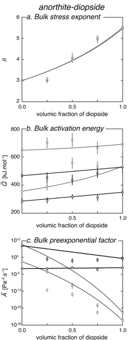
Bulk viscosities have been calculated with stress exponents of 1 for both anorthite and diopside in the dif-fusion creep regime and higher values in the dislocation creep regime (anorthite: n = 3, diopside: n = 5.5 [Dimanov and Dresen, 2005]). The predicted evolution is logarithmic for the diffusion experiments (Figures 4a and 4b) and is convex up for the dislocation experiments (Figures 4c and 4d). Thus, even if the difference between the predicted and the experimental viscosity is generally less than half an order of mag-nitude, the MPG model fails to reproduce the experimental S-shape trend. More precisely, it overestimates the viscosity for the diopside fractions of 0.25 and 0.5 and underestimates it for the diopside fraction of 0.75. The experimental data in the diffusion creep regime are consistent with bulk stress exponents of 1 for anorthite, diopside, and aggregates of intermediate composition. This is predicted by the MPG model (see Table 2). In the dislocation creep regime, the experimental and predicted bulk stress exponents are in good agreement even if the model does not reproduce the smooth S-shape experimental trend (Figure 5a). The experimental values of the bulk activation energy are well reproduced by the predicted one for the diffu-sion creep regime and the dry dislocation creep regime (Figure 5b). The agreement is, however, not as good for the wet dislocation creep regime. For the bulk preexponential factor (Figure 5c), the agreement between experimental and predicted values varies from very good (wet diffusion creep) to very poor (dislocation

Figure 5. (a–c) Bulk creep parameters of

anorthite-diopside aggregates as a function of the frac-tion of diopside: comparison between the experimental data set of Dimanov and Dresen [2005] (open symbols) and the predictions of the MPG model (solid curves). The black (resp. grey) color corresponds to diffusion (resp. dislocation) creep experiments. Open circles (resp. squares) correspond to wet (resp. dry) conditions. The vertical bars correspond to the fitting errors calculated during the regression of the creep parameters.

creep). Since the stress exponent is regressed first and the preexponential factor is regressed third, the decrease in the agreement between experiments and predictions, from stress exponent to preexponential factor, might be an artifact of the regression process of the creep parameters. Small errors in the deter-mination of the bulk stress exponent and activation energy might lead to large errors in the determination of the bulk preexponential factor.

5.5. Halite-Calcite Aggregates

In the experiments of Jordan [1987] and [Bloomfield

and Covey-Crump 1993], calcite is 1 order of

mag-nitude stronger than halite (Figure 6a). Calcite deformed partly by intracrystalline plasticity with twinning and partly by cataclasis, whereas halite deformed by dislocation glide. The experimental vis-cosities show a logarithmic increase with increasing calcite fraction. The predictions of the MPG model have been calculated with stress exponents deter-mined in other experimental studies (halite: n = 5.3 [Carter et al., 1993], calcite: n = 7.8 [Schmid et al., 1980]). For both experimental data sets, the values calculated with the MPG model reproduce the exper-imental values very well, even if cataclastic flow of calcite which is not strictly modeled by a power law was active in the experiments.

5.6. Calcite-Anhydrite Aggregates

In the experiments of Barnhoorn et al. [2005], cal-cite and anhydrite have viscosities of the same order of magnitude (Figure 6b). They deformed (sepa-rately and together) in the dislocation creep regime with exception of one experiment (70% of anhy-drite) where anhydrite deformation was controlled by diffusion creep or grain boundary sliding. The viscosity measured in a torsion apparatus (used for these experiments) depends on the stress exponent of the material. Barnhoorn et al. [2005] suggest that 5is the most likely value for the stress exponent of most of the aggregates. In the aggregates having a calcite-anhydrite ratio of 1:1, their preferred value is 3. The dispersion due to variations of stress exponent between 1 and 5 is shown, in addition to the exper-imental viscosity values (Figure 6b). The viscosity of the aggregate containing 70% of anhydrite is lower than the viscosity of the two end-members, which is due to a change in the deformation mechanism of anhydrite. This data point is therefore not considered here. The predictions of the MPG model have been calculated with a stress exponent of 5 for both calcite and anhydrite. Variation of the end-member stress exponent induces a minor dispersion of the predicted viscosity (grey background on Figure 6b). If the outlier value is not considered, the predicted values are very similar to the experimental data.

5.7. Octachloropropane-Camphor Aggregates

Octachloropropane (OCP) and camphor are crystalline organic materials that creep at room temperature and low stress. In the three constant load experiments of Bons and Urai [1994], the viscosity shows the

Figure 6. (a) Viscosity of halite-calcite aggregates as a function of the fraction of calcite: comparison between the exper-imental data sets of Jordan [1987] (grey open circles) and Bloomfield and Covey-Crump [1993] (black open circles), on the one hand, and the predictions of the MPG model (solid curves), on the other hand. The viscosity corresponds to 10% strain for Jordan [1987] experiments and 20% strain for Bloomfield and Covey-Crump [1993] experiments. Bulk strain rate: 10−5_s−1_{, temperature: 473 K, confining pressure: 200 MPa. (b) Viscosity of calcite-anhydrite aggregates as a} func-tion of the fracfunc-tion of anhydrite: comparison between the experimental data set of Barnhoorn et al. [2005] (open circles) and the predictions of the MPG model (solid curves). The vertical bars indicate the range in viscosity due to variations of the end-member stress exponents between 1 and 5. The grey background indicates the range in predicted viscosity due to the variations of the end-member stress exponent. The viscosity corresponds to the peak stress (shear strain of approximately 0.5). Bulk strain rate: 10−3_s−1_{, temperature: 1873 K, confining pressure: 300 MPa.}

same parallel evolution. It increases regularly over 3 orders of magnitude with increasing camphor fraction (Figure 7a). Predictions with the MPG model have been calculated with the stress exponents derived from the stepping load experiments (OCP: n = 4.5, camphor: n = 3.3). The three predicted viscosity curves are also parallel and follow the experimental trend. However, the predictions slightly overestimate the experimental values with a maximum difference of approximately half an order of magnitude.

The bulk stress exponent and bulk constant factor of OCP-camphor aggregates have been determined with stepping load experiments at constant temperature [Bons and Urai, 1994]. The stress exponent values of the aggregates of intermediate composition are close to the one of OCP (Figure 7b). Furthermore, the bulk stress exponent shows a bell-shape evolution with increasing camphor fraction. This increased nonlinearity might be the effect of grain-scale mechanical interactions between OCP and camphor grains. This is probably why the predictions of the MPG model fail to reproduce both the experimental values and trend. The experi-mental bulk constant factor (which includes the preexponential factor and the thermal part of the power law) decreases regularly with the increasing camphor fraction (Figure 7c). The predicted evolution of the bulk constant factor reproduces the experimental trend. However, the predictions slightly underestimate the experimental values, which is consistent with the overestimation of the viscosity (Figure 7a). Because of the surprising evolution of the bulk stress exponent, the very weak OCP has been suggested to control the deformation of the aggregate, even at large camphor contents [Bons and Urai, 1994]. This mechanical con-trol is not in line with the regular experimental evolution of the bulk viscosity (Figure 7a) and bulk constant factor (Figure 7c) reproduced by the MPG model.

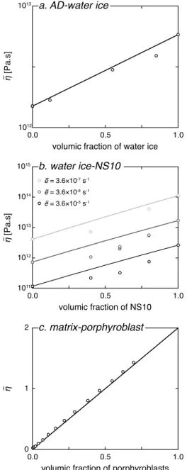
5.8. Ammonia Dihydrate-Water Ice Aggregates

In the experiments of Durham et al. [1993], both ammonia dihydrate (NH₃⋅ 2H2O) and water ice deformed by dislocation creep. Water ice was 1 order of magnitude stronger than ammonia dihydrate (Figure 8a). The viscosity value for pure ammonia dihydrate (open square on Figure 8a) was deduced by Durham

et al. [1993] from the experimental data set with the mixing model of Tullis et al. [1991]. Even without

this model-dependent point, the evolution of bulk viscosity with increasing water ice content is close to logarithmic. The viscosity predicted by the MPG model are calculated with the stress exponents deter-mined by Durham et al. [1993]. The predictions of the MPG model slightly overestimate the experimental data. Another value for the poorly constrained viscosity of pure ammonia dihydrate (which could not be synthesized) could lead to an even better agreement.

Figure 7. (a–c) Viscosity and bulk creep parameters of octachloropropane (OCP)-camphor aggregates as a func-tion of the fracfunc-tion of camphor: comparison between the experimental data set of Bons and Urai [1994] and the predictions of the MPG model (solid curves). The vertical bars correspond to the fitting errors calculated during the regression of the creep parameters. Temperature: 301 K, confining pressure: 0.6 MPa.

5.9. Water Ice-Sodium Sulfate Hydrate Salt Aggregates

In the experiments of Durham et al. [2005], both water ice and sodium sulfate hydrate salt (Na2SO4.10H2O, NS10) deformed in the dislocation creep regime. NS10 had a viscosity 1 order of magnitude larger than water ice calculated using the parameters for pure ice I [Durham and Stern, 2001] (Figure 8b). The predic-tions of the MPG model, which are calculated with the end-member viscosities and the stress exponent of water ice (n = 4 [Durham and Stern, 2001]) and NS10 (n = 5.4 [Durham et al., 2005]), systematically overes-timate the viscosity of the aggregates by half an order of magnitude (Figure 8b). Further, the experimental values have a convex-up trend, whereas the predicted curve is convex down. Note, however, that the values for pure ice come from another experimental data set [Durham and Stern, 2001].

5.10. Matrix-Porphyroblast Numerical Aggregates

Several numerical studies have been published on the topics of two-phase aggregates. Here we only consider the study of Groome et al. [2006], since the other studies either have too little experimental data [Tullis et al., 1991; Madi et al., 2005], or consider very simplified geometries [Treagus and Lan, 2000; Takeda

and Griera, 2006], or deal with anisotropic viscosities

that cannot be treated with our approach [Treagus, 2003; Dabrowski et al., 2012].

Groome et al. [2006] studied the mechanical effect of

strong porphyroblasts (dimensionless linear viscos-ity of 100) growing in a weak matrix (dimensionless linear viscosity of 1). The numerical experiments were performed under simple shear boundary condi-tions. The bulk viscosity of the numerical aggregates shows a close to logarithmic increase with increas-ing porphyroblast fraction (Figure 8c). The evolution predicted by the MPG model is perfectly logarith-mic, since linear viscous materials are considered (see equation (48)). The agreement between the numerical experiment and the predictions is excellent.

6. Comparison With Other Mixing Models

The MPG model makes good predictions of the bulk viscosity and the bulk creep parameters for the most of the two-phase experiments. Here a qualitative and quantitative comparison is made between the MPG model and nine representative mixing models from the literature.

6.1. Qualitative Comparison

Three classes of models are distinguished.

6.1.1. The Bounding Models

The first class of models provides bounds for the viscosity of a polyphase aggregate. The Reuss lower and Voigt upper bounds are respectively calculated as the weighted harmonic and arithmetic means of the

Figure 8. (a) Viscosity of ammonia dihydrate (AD)-water ice aggregates as a function of the fraction of water ice: comparison between the experimental data sets of Durham et al. [1993] (open circles) and the predic-tions of the MPG model (solid curves). Bulk strain rate: 3.5 10−6_s−1_{, temperature: 167 K, confining pressure:} 50 MPa. (b) Viscosity of water ice-sodium sulfate hydrate salt (NS10) aggregates as a function of the fraction of NS10: comparison between the experimental data sets of Durham and Stern [2001] (open circles) and the pre-dictions of the geometric mixing models (solid curves). Bulk strain rate of 3.5 10−5_{, 3.5 10}−6_{, and 3.5 10}−7_s−1_, temperature: 233 K, confining pressure: 50 MPa. (c) Adimensioned viscosity of numerical aggregates of strong porphyroblasts embedded in a weak matrix as a function of the fraction of porphyroblasts: compari-son between the numerical experiments of Groome et

al. [2006] (open circles) and the predictions of the MPG

model (solid curve).

phase viscosities [Voigt, 1928; Reuss, 1929]. Both are valid for layered aggregates of linear viscous mate-rial deformed with special boundary conditions. The mixing models for “interconnected weak layer” and “load-bearing framework” microstructures [Handy, 1994a, 1994b] lead to values which are close to these bounds. Theoretically, the bulk viscosity of any aggre-gate must lie between the Reuss and Voigt bounds [Markov, 1999]. Violations of the Reuss lower bound have, however, been reported [Tullis and Wenk, 1994;

Bruhn et al., 1999]. They are interpreted to be the

result of anisotropies, grain growth inhibition, or enhanced diffusion along the grain boundaries. Refined bounds have been proposed for power law materials [Zhou, 1995]. They are calculated by min-imizing the power under constraints of arithmetic strain rate or stress partitioning. These bounds which were originally calculated numerically have been revised in this paper and correspond to the semiana-lytical MPA models (Zhou lower bound: MPAe model, Zhou upper bound: MPAs model). The analysis of these models (see section 4.3) reveals that the MPAe (resp. MPAs) model leads to an almost homogeneous stress (resp. strain rate) in the aggregate. This suggests that the Zhou bounds must generally lie close to the Reuss and Voigt bounds.

The bounding models predict evolutions which are either convex up or convex down (Figure 9a). A sharp increase of the viscosity with increasing fraction of the strong phase is also predicted at approximately 0.2 fraction of the strong phase for the upper bounds and at approximately 0.8 fraction of the strong phase for the lower bound. Such predictions are not con-sistent with either the almost logarithmic evolution of the viscosity or the S-shape trend which have been identified in most experimental data sets (see section 5). However, the lower bounds might pro-duce good approximations when the microstructures are weak-phase supported until large fractions of the strong phase are present.

6.1.2. The Geometric Models

The second class of models is based on a geometric averaging procedure. The geometric mean (GM on Figure 9b) is one particular case of the general-ized mean model [Ji, 2004]. The use of such a mean has no physical basis. It can, however, be considered as a good approximation for two-phase aggregates [Ji, 2004]. It also provides good results for averaging the elastic properties of aggregates [Matthies and

Humbert, 1993; Mainprice and Humbert, 1994]. Tullis et al. [1991] proposed an empirical mixing

model for aggregates of two power law materials. This assumes that the bulk behavior also follows a power law with a bulk stress exponent calculated as

Figure 9. (a) Bulk viscosity of anorthite-diopside aggregates as a function of the diopside fraction predicted by the MPG model, the Voigt and Reuss bounds, the Zhou lower and upper bounds, and the self-consistent model for 2-D geome-try (SCM2) [Treagus, 2002, equation (9)] and for 3-D geomegeome-try (SCM3) [Treagus, 2002, equation (22)]. (b) Bulk viscosity of anorthite-diopside aggregates as a function of the diopside fraction predicted by the Minimized Power Geometric (MPG) model, the geometric mean (GM), and the first and second Ji models. Predictions are calculated for temperature of 1023 K and strain rate of 10−16_s−1_{. The creep parameters of anorthite and diopside correspond to the dislocation creep} regime in wet conditions [Dimanov and Dresen, 2005]. Also shown is the viscosity calculated with the creep parameters determined for aggregates of intermediate composition (open circles). The good fit between the experimental data and the SCM model is here exceptional (see section 6.2).

the weighted geometric mean of the end-member stress exponents. This model also assumes that the bulk viscosity at a given temperature is equal to the isoviscous point of the two end-members.

Other power law models based on geometric averaging have also been proposed by Ji and Zhao [1993] and Ji et al. [2003]. The first Ji model (Ji1 on Figure 9b) assumes a homogeneous stress in the aggregate and geometric strain rate partitioning, while the second Ji model (Ji2 on Figure 9b) assumes homogeneous strain rate and geometric stress partitioning. Since neither a homogeneous strain rate nor a homogeneous stress are generally realistic [Tullis et al., 1991], iterations can be used to find a more accurate model [Ji and

Zhao, 1993; Ji et al., 2003]. Results of this iterative procedure are almost identical to those of the Tullis et al.

[1991] model [Ji and Zhao, 1993; Ji et al., 2003].

All the geometric models predict the same close to logarithmic evolution with very similar viscosities (Figure 9b). The MPG model belongs to this group.

6.1.3. The Self-Consistent Model

The self-consistent model (SCM) approximates an aggregate of two linear elastic phases as a homogeneous aggregate made of an ellipsoidal inclusion embedded in a matrix [Budiansky, 1965; Hill, 1965; Jiang, 2013]. This model can also be applied to linear viscous materials [Treagus, 2002]. Amongst all the mixing mod-els considered here, the SCM is the only one which is based on Newton’s equation of motion. It predicts an S-shape curve with an inflection point at 0.4 strong phase fraction for 3-D geometry and 0.5 strong phase fraction for 2-D geometry (Figure 9a). Even if the SCM is not based on a transition between weak- and strong-phase supported microstructures, it could be a good approximation for such a transition.

Models for nonlinear viscous materials have also been developed using a self-consistent approach [Duva, 1984; Yoon and Chen, 1990]. They are not considered here because they assume that the strong phase of the aggregate is rigid. This results in unrealistic viscosities for aggregate compositions close to the strong end-member.

6.2. Quantitative Comparison

The ability of all the 10 models to reproduce the 15 experimental data sets presented in section 5 is assessed in a quantitative way. For each set of experimental data set and mixing model, two misfits are calculated (see Appendix B for their definitions). The mean standard deviation misfit, Δ̄𝜂, estimates the order of mag-nitude of the absolute misfit between experimental and predicted bulk viscosities. The mean misfit,𝛿 ̄𝜂, estimates the order of magnitude of the relative misfit between experimental and predicted bulk viscosities. The smaller the absolute value of the misfits are, the better the fit is. Absolute values of Δ̄𝜂 and 𝛿 ̄𝜂 of 0.2, 0.4, and 1 indicate that the ratio between the experimental viscosities and the predicted ones is on average