Optimizing Molecular Cloning of Multiple Plasmids

HAL Id: hal-01628328

https://hal.archives-ouvertes.fr/hal-01628328

Submitted on 3 Nov 2017

HAL is a multi-disciplinary open access

archive for the deposit and dissemination of

sci-entific research documents, whether they are

pub-lished or not. The documents may come from

teaching and research institutions in France or

abroad, or from public or private research centers.

L’archive ouverte pluridisciplinaire HAL, est

destinée au dépôt et à la diffusion de documents

scientifiques de niveau recherche, publiés ou non,

émanant des établissements d’enseignement et de

recherche français ou étrangers, des laboratoires

publics ou privés.

Optimizing Molecular Cloning of Multiple Plasmids

Thierry Petit, Lolita Petit

To cite this version:

Thierry Petit, Lolita Petit. Optimizing Molecular Cloning of Multiple Plasmids. International Joint

Conference on Artificial Intelligence, 2016, Buenos Aires, Argentina. p. 773-779. �hal-01628328�

Optimizing Molecular Cloning Of Multiple Plasmids

Thierry Petit

Foisie School of Business,

Worcester Polytechnic Institute, USA

tpetit@wpi.edu

thierry.petit@mines-nantes.fr

Lolita Petit

Gene Therapy Center,

University of Massachusetts Medical School,

Worcester MA, USA

lolita.petit@umassmed.edu

Abstract

In biology, the construction of plasmids is a rou-tine technique, yet under-optimal, expensive and time-consuming. In this paper, we model the Plas-mid Cloning Problem (PCP) in constraint program-ing, in order to optimize the construction of plas-mids. Our technique uses a new propagator for the AtMostNVector constraint. This constraint al-lows the design of strategies for constructing mul-tiple plasmids at the same time. Our approach rec-ommends the smallest number of different cloning steps, while selecting the most efficient steps. It provides optimal strategies for real instances in gene therapy for retinal blinding diseases.

1

Introduction

Construction of plasmids is one of the most commonly used techniques in molecular biology. Invented 40 years ago, this technique led to impressive applications in medicine and biotechnologies, such as the production of large amounts of insulin and antibiotics in bacteria, as well as the manipula-tion of genes in host organisms. In most cases, plasmids are constructed by cutting and assembling DNA fragments from different sources [Brown, 2010]. However, the physical as-sembly of DNA parts is a time-consuming process for the ex-perimenter, as it requires a multitude of steps. Minimizing the number of different steps that are necessary to build multiple plasmids at the same time can significantly reduce laboratory work time and financial costs.

In this paper, we introduce a Constraint Programming (CP) approach to the Plasmid Cloning Problem (PCP). The ob-jective of the PCP is to recommend the smallest number of different cloning steps, while selecting the most efficient steps. For this purpose, we design a constraint model and we introduce a new propagator for the AtMostNVector con-straint [Chabert et al., 2009]. We show that no dominance properties exist between our technique and state-of-the-art propagators. This complementarity is confirmed empirically. We demonstrate the relevance of using an Artificial Intelli-gence framework for modeling the PCP by successfully solv-ing real instances in gene therapy for retinal blindsolv-ing diseases.

∗

This work was partially supported by the Fulbright-Fondation Monahan, Fondation de France and AFM T´el´ethon fellowships.

The remainder of this paper is organized in the following manner. Section 2 describes the PCP. Section 3 introduces a CP model for the PCP and a new propagator for AtMost-NVector, theoretically and empirically evaluated. Section 4 presents experiments on real PCP instances.

2

The Plasmid Cloning Problem

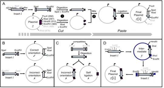
Construction of plasmids refers to the isolation of an oriented DNA sequence containing a gene of interest, insert, and its in-sertion into a circular molecule, plasmid, which can be used to generate multiple copies of the DNA when introduced into host cells (Fig. 1, next page). Each insert i is typically en-closed into two different plasmids, z test and z cont (con-trol), to yield two final plasmids z test [i] and z cont [i].

Inserting the insert into a plasmid is generally performed using a cut and paste approach (Fig. 1A). First, the insert and the plasmid are cut with commercially available restriction enzymes (e.g., [Biolabs, 2015c]) at specific restriction sites in order to generate compatible ends. Then, digested DNA fragments are mixed together to allow their compatible ends to anneal to each other. A DNA ligase is added to the solution to covalently join the two fragments.

The most crucial part of the experiment is to determine how the insert is introduced into the plasmids, i.e., which pairs of restriction enzymes will be used to cut the insert and the plas-mids to facilitate the cloning. The PCP considers the con-struction of multiple plasmids at the same time. We cannot select enzymes recognizing restriction sites that are already present within the insert or present more than once in the plas-mid. Using an enzyme recognizing any of these sites would provoke fragmentation of DNAs. The list and positions of re-striction sites present within each DNA sequence can be gen-erated by several analysis DNA software tools, e.g., [ApE, 2015]. Let z be either z test or z cont , and z[i] the result-ing final plasmid. Let the integer identifiers x[i].before and x[i].after be the restriction sites located at ends of insert i to allow its cloning into z. Five constraints apply:

(A) Enzymes used to cut the insert i and the plasmid z need to create identical or equivalent ends, as only physically compatible ends can be covalently ligated (Fig. 1A). Therefore, the restriction sites x[i].before and x[i].after should be compatible with the restriction sites of z[i]. The list of enzymes creating compatible ends is freely

Insert i XbaI (297) HindIII (312) EcoRV (383) XhoI (499) Plasmid z

NotI EcoRV _Digestion

Digestion x[i].before x[i].after 1 2 Mix 3 Ligation _Final Plasmid z[i] SpeI XbaI EcoRV Cut Paste A B

SpeI EcoRV Correct

orientation ✓ SpeI XbaI EcoRV Incorrect orientation ✗ SpeI XbaI EcoRV EcoRV SpeI 0 C Incorrect orientation ✗ Self ligation ✗ PvuII EcoRV SpeI XhoI (876) XhoI XhoI PvuII (292) [i].before XbaI EcoRV PvuII Inter-mediate y DraI XhoI PvuII HindIII EcoRI D XbaI EcoRV PvuII EcoRI HindIII Final Plasmid z[i] SpeI + EcoRV XbaI + EcoRV Insert i Insert i Insert i Insert i Digestion compatibles

Figure 1: Construction of plasmids using the digestion/ligation method. (A) General procedure for cloning an insert into a plasmid. Using polymerase chain reaction, restriction sites (SpeI and EcoRV in this example) are added at both ends of an oriented insert i (arrow). The insert and the plasmid are digested by restriction enzymes to generate sticky and complimentary ends. With the addition of DNA ligase, the insert and the plasmid recombine at the sticky end sites. The result is a new plasmid containing the insert. (B)-(D) Orientation and compatibility constraints for the cloning of an insert into a final plasmid, in one step (B), (C), or when an intermediate plasmid is required (D). Restricted sites that are excluded are in grey. Restriction site position in the plasmid is given in parenthesis.

provided by suppliers, e.g., [Biolabs, 2015a]. Moreover, in some cases, ligation of two compatible ends can de-stroy both original restriction sites in the hybrid DNA sequence. These sites are excluded from the list to allow the experimenter to easily remove or exchange the insert from the final plasmid, should this be required.

(B) The insert must be enclosed into the plasmid in the right orientation to allow its expressivity. As restriction sites present in the plasmid z are totally ordered by their posi-tion, the two enzymes used to cut the insert i, x[i].before and x[i].after , should recognize restriction sites with identical orientation on the plasmid z[i] (Fig. 1B). In addition, in z[i], the restriction sites should be separated by d (a positive integer), as many restriction enzymes do not cut DNA efficiently at the end of a DNA sequence. Therefore, we must have z[i].before + d < z[i].after . (C) Enzymes used to cut the two ends of the insert and

plas-mid should raise two different and not compatible ends. Otherwise, the insert could be assembled to the plasmid in either the correct or incorrect orientation. Addition-ally, the plasmid may self-ligate omitting the insert (Fig. 1C). Consequently, x[i].before should not be compatible with x[i].after ; the same for z[i].before and z[i].after . (D) Many assembling strategies cannot be done in only one

cloning step. If and only if no direct solutions exist, a plasmid y containing different restriction sites will be used to generate an intermediate construct y[i]. The in-sert i can be fused in either orientation into the interme-diate plasmid y, but the correct orientation of the insert i needs to be restored when cloned into the final plasmid z (Fig. 1D). Note that in this case four steps are necessary:

1) digest insert i to generate ends compatible with y, 2) assemble i and y, 3) extract i from y[i] to generate ends compatible with z and 4) ligate i and z to get z[i]. (E) As using an intermediate plasmid is very time

consum-ing task for the experimenter, we constrain x[i].before and x[i].after to be identical for the construction of both z test and z cont when an intermediate plasmid is re-quired for the construction of both z test and z cont . Optimization criteria. When multiple plasmids are con-structed at the same time, sharing the same cloning strat-egy reduces the total step count, associated laboratory work and reagent costs, because plasmid digestion and purification steps can be done in parallel. Therefore, our primary objec-tive is to minimize the number of distinct pairs of enzymes (z[i].before, z[i].after ) used to construct all final plasmids. In addition, not all pairs of restriction enzymes (before, after ) are equivalent in practice. Restriction enzyme cost is stem from buffer and temperature compatibility, as well as cloning efficiency. In particular, it is highly desirable that at least one of the restriction enzyme generates a sticky-end DNA frag-ment because the ligation is easier when there are overhangs. Our second objective is to determine optimized pairs of re-striction enzymes to perform the selected cloning steps. Pref-erence is given to low costs. Properties of each enzyme are provided by the supplies, e.g., [Biolabs, 2015b].

Related work. To our knowledge, no existing software can solve the PCP. We emphasize that emerging techniques and software have been designed for optimizing the construc-tion of genetic composites from a set of predefined DNA

parts [Appleton et al., 2014; Casini et al., 2015; Densmore et al., 2010]. Although the research area is common with our application, constraints fundamentally differ from the PCP. In related studies, the authors assemble multiple DNA frag-ments together, but restriction sites are predefined and fixed.

3

Constraint Model

In Constraint Programming (CP), constraints state relations between variables. A set of constraints forms a model of a constraint problem. Each variable has a finite domain of pos-sible values. In this paper we consider exclusively integer do-mains. An assignment of values to variables is an instantia-tionif and only if each value belongs to the domain of its vari-able. Constraints are associated with propagators. Through embedded filtering algorithms, a propagator removes domain values that cannot be part of a solution to a constraint. Do-main reduction can be more or less effective. A propagator is GAC (Generalized Arc Consistent) if and only if it removes all the values that cannot satisfy the constraint. In this paper, we use the AtMostNVector constraint [Chabert et al., 2009]. Definition 1 (AtMostNVector). Let V be a collection of k vectors of variables, V = [X(0)_{, X}(1)_{, . . . , X}(k−1)_{]. Let}

obj be an integer variable. Each X(a)_{containsp variables,}

X(a)= {x(a)₀ , x(a)₁ , . . . , x(a)_p−1}. Two vectors X(a)_andX(b)

are distinct if and only if∃ j ∈ {0, 1, . . . , p − 1} such that x(a)_j 6= x(b)_j . We use the notationnb6=(V ) for the number of

distinct vectors within an instantiation of all variables in V. AtMostNVector(V, obj ) ⇔ nb6=(V ) ≤ obj .

As many CP problems are NP-Hard, a search procedure is required. The search process can be systematic, e.g., a Branch and Bound scheme, or not, e.g., Large Neighborhood Search.

3.1

Constraint model for the PCP

CP is a good candidate for the PCP because efficient prop-agators exist for table constraints [Lecoutre et al., 2015; Perez and R´egin, 2014; Mairy et al., 2014]. They can be combined with more specific constraints, such as AtMost-NVector. A table constraint is defined by the set of combi-nations of values that satisfy it (or, respectively, violate it), called tuples. In our model, due to intricate rules on enzyme pairs, all constraints except objective constraints are tables. The issue is to find the good tradeoff between arity (number of variables in each table) and propagators running time. Do-main reduction is better with a high arity but the number of tuples may become huge and the filtering algorithms exces-sively time consuming. We present the best found model, in terms of solving capabilities. We provide solutions with sites that were initially present in their plasmid. A component c is a triplet of variables hc.before, c.after , c.cost i. We distinguish three “layers” of components. For each insert i we state:

• One component x[i]. If at least one intermediate is re-quired to ligate the final plasmids test and/or control, this component represents the pairs of enzymes used to cut the insert, with respect to test and/or control. We can de-termine whether at least one direct solution exists or not before solving the problem by comparing all site pairs. This modeling structurally guarantees that constraints

(E) of Section 2 is satisfied, as if there are two inter-mediate they share the same component x[i]. Domains of x[i].before and x[i].after are generated from lists of candidate sites. In agreement with biologists, cost do-main is D(x[i].cost ) = {0, 1, 2, 4, 6}.

• Two components y p test[i] and y p cont[i] that repre-sent site pairs that will match to x[i] in the intermediate plasmid when no direct solution exist for i, and site pairs used to cut the insert otherwise. In the case of use of an intermediate plasmid, more than one intermediate can-didate may exist in data. We merge in the domains the sites of all candidates. Cost domains are {0, 1, 2, 4, 6}. • Two integer variables, ind y test[i] and ind y cont[i],

whose domains are the set of all unique identifiers for plasmid candidates, plus value −1 to deal with the case where no intermediate plasmid is used.

• Two components z test[i] and z cont[i] that represent the pair of sites selected in the target plasmid. Domains are generated similarly to x[i].

In addition, we define two objective variables, one for the number of distinct vectors in target plasmids, obj nvector , and one for the sum of costs, obj sumcost .

The table constraints are the following. Recall that consistent pairs of enzymes and their cost and position are data. Suffix C is used to state a constraint on costs and string test for test inserts/plasmids. We present only test plasmids constraints: to add constraints on control plasmids in the model, just duplicate all constraints with string test and replace test by cont. For each i we define:

X C(x [i ].before, x [i ].after , x [i ].cost )

Yp test C(y p test [i ].before, y p test [i ].after , y p test [i ].cost ) Yc test C(y c test [i ].before, y c test [i ].after , y c test [i ].cost ) Z test C(z test .before[i ], z test [i ].after , z test [i ].cost ) XY test(x [i ].before, x [i ].after , ind y test [i ],

y p test [i ].before, y p test [i ].after )

YY test(ind y test [i ], y p test [i ].before, y p test [i ].after , y c test [i ].before, y c[i ].test after )

YZ test(y c test [i ].before, y c.test [i ].after , z test [i ].before, z test [i ].after )

We now summarize the generation of allowed tuples in tables, according to the PCP constraints A,B,C,D and E detailed in Section 2, and describe the optimization scheme. Cost constraints. Concerning X C, if no intermediate plas-mid is used both for test and control (E), tuples (v, w, 0) are generated for each (v, w) in D(x[i].before) × D(x[i].after ). Otherwise, cost c of each pair is stem from data and the tuple (v, w, c) is added accordingly. Yp test C is similar to X C. Tables Yc test C and Z test C are similar to X C but simpler, as exclusively tuples of the form (v, w, c) are added.

Transition constraint XY test. If no intermediate is re-quired, we add all tuples (v,w,-1,t,u) to the table, according to the variable domains. Otherwise, depending on the intermediate plasmid identifier id , we generate valid tuples (v,w,id ,t,u) restricted so as: t and u must be enzymes of the intermediate plasmid id ; v and w must not be compatible or equal (C); t and u must not be compatible or equal (C); v and t must be compatible or equal (A); w and u must be compatible or equal (A); t and u must be distant from d (B). Transition constraint YY test. If no intermediate is re-quired, we add all valid possible tuples (-1,t,u,t,u) subject to

the following rules: t and u must not be compatible (C); t and u must belong to the insert domain (E). Otherwise, we add tuples (id ,t,u,r,s). t,u,r and s must be enzymes of the intermediate candidate id ; t and u must not be compatible or equal (C); r and s must not be compatible or equal (C); Moreover, two cases should be considered. (1) position of t < position of u. The direction is correct and position of r should be ≤ position of t, while position of s should be ≥ position of u (B and D). (2) position of t > position of u. A re-inversion is required, position of r should be ≤ position of u, while position of s should be ≥ position of t (B and D). Transition constraint YZ test. Tuples should preserve ends compatibility (A) and distance between enzymes in each component (B), similarly to XY test.

Objective constraints and optimization scheme. An instance of AtMostNVector(V, obj nvector ) defines the first objective, such that V = {(z test [0].before, z test [0].after ), (z test [1].before, z test [1].after ),. . .} ∪ {(z cont [0].before, z cont [0].after ),(z cont [1].before, z cont [1].after ),. . . }. We minimize obj nvector , fix this variable to the best found value and then minimize the sum of all cost variables, obj sumcost . Then, increase obj nvector by one and minimize again obj sumcost . Other points in the Pareto can be obtained by relaxing more obj nvector , if needed. Best obj nvector value can be found using a bottom-up scheme: try to find a solution with one distinct vector, if there is no solution then try with two distinct vectors, and so on. The solution is optimal providing that proofs of lack of solutions with lower objective values have been made.

3.2

Propagating AtMostNVector

AtMostNVector was introduced in the context of simultane-ous localization and map building (SLAM) [Chabert et al., 2009] and can be used in many contexts, including biol-ogy [Grac¸a et al., 2009; Backeman, 2013]. Proving that the minimum value in the domain of obj variable can be part of a solution of AtMostNVector is NP-Hard [Chabert et al., 2009]. Therefore, enforcing GAC on AtMostNVector is NP-Hard, as well as Bounds-consistency1 _{[Backeman, 2013]. With}

respect to AtMostNValue, the particular case of AtMost-NVector with vectors of one variable, filtering algorithms lighter than GAC have been introduced, using Linear Pro-gramming and Lagrangian Relaxation [Bessi`ere et al., 2006; Cambazard and Fages, 2015] and Favaron et al.’s approxi-mation of a maximum independent set on the compatibility graph [Favaron et al., 1993; Bessi`ere et al., 2006]. In the compatibility graphG of a set of vectors V of size k, each node represents a vector from V and there is an edge between two nodes if and only if the corresponding vectors can be equal, given the current domains. An independent set is a set of nodes where no two nodes in the set are connected by an edge. A maximum independent set is an independent set of maximum cardinality. Finding this set is NP-Hard. The car-dinality can be approximated, given m the number of edges in G: obj ≥l2k−

2m d2m/ke d2m/ke+1

m

. Backeman has shown that the filter-ing techniques based on this lower-bound of obj for the

con-1

i.e., considering that domains are represented by their minimum and maximum value and have no holes.

1 card := Cardinalities of values in each row of vec; 2 scard := Sort each row of card in ascending order; 3 int res := 1;

4 for j ∈ {0, 1, . . . , p − 1} do

5 nbco := 0; cur := 0; i := scard[j].length − 1; 6 while nbco < k do

7 nbco := nbco + scard[j][i];

8 i := i − 1; cur := cur + 1;

9 res := max(res, cur );

10 return res;

Algorithm 1: NVECTORLB.

straint AtMostNValue [Bessi`ere et al., 2006] can be adapted to the case of AtMostNVector [Backeman, 2013].

Cardinality-Based Propagator. We suggest a new tech-nique for improving G-based propagators. Researchers in bi-ology should not have to determine the appropriate parame-ters or combination of algorithms, e.g., the sub-gradient algo-rithm in a Lagrangian relaxation based technique. We must consider a black-box approach. Whereas existing propagators are based on pairwise comparisons of vectors, through the edges of G [Backeman, 2013], we consider the set of variables at a given vector position. For each j ∈ {0, 1, . . . , p − 1}, we consider the variables {x(0)_j , x(1)_j , . . . , x(k−1)_j }. Every vari-able in this set belongs to a different vector.

Definition 2. Let X be a set of variables and v a value. The cardinality#v of v is the number of domains of variables in X that contain v.

If the maximum cardinality among all values in the union of domains of variables {x(0)_j , x(1)_j , . . . , x(k−1)_j } is strictly less than k, then at least two vectors will be distinct. If the sum of the two maximum cardinalities is strictly less than k, then at least three vectors will be distinct, and so on. Among all j ∈ {0, 1, . . . , p − 1}, the maximum required distinct vectors is a lower bound for obj . Let minv the minimum value among all domains and maxv the maximum one. Let r = maxv − minv + 1. To compute this lower-bound, Algorithm 1 uses the global variables: card : p × r integers matrix that is used to store cardinalities of values (sorted in scard ); vec: k × p matrix of variables that rep-resents [X(0), . . . , X(k−1)_{]; We assume that the solver raises}

an exception when a domain is emptied. As a consequence, in Algorithm 1 we cannot have a sum of occurrences of the values in domains strictly less than the number of variables. Property 1 (Correctness). Let vec be a k × p integer variable matrix. Algorithm 1 returns a lower bound of the number of distinct vectors in the matrix.

Proof. scard[j] is the set of value cardinalities of column j of vec, j ∈ {0, 1, . . . , p − 1}, sorted in ascending order. Start-ing from the last cell in scard[j], while nbco < k, the algo-rithm (line 6) iterates on maximum cardinalities and counts covered variables in column j of vec, through nbco (line 7). The number of iterations is by construction a lower bound of the number of distinct values in any instantiation of column j

1 obj := NVECTORLB(vec, card ); // Fill card

2 for i ∈ {0, 1, . . . , k − 1} do 3 for j ∈ {0, 1, . . . , p − 1} do

4 for v ∈ D(vec[i][j]) do

5 Decrease by 1 v cardinality in card [j];

6 scard [j] := Sort card [j] in ascending order; 7 nbco := 0; lb := 0; idx := scard[j].length − 1; 8 while nbco < k and idx > 0 do

9 nbco := nbco + scard[j][idx];

10 lb := lb + min(1, scard[j][idx]);

11 idx := idx − 1;

12 if lb > obj ∨ (lb = obj ∧ nbco < k) then

13 for v ∈ D(vec[i][j]) do

14 once := True;

15 nbco := 0; cur := 0;

idx := scard[j].length − 1;

16 while nbco < k do

17 nbco := nbco + scard[j][idx];

18 if scard[j][idx] = cardinality of v in

card [j] and once then

19 nbco := nbco + 1;

20 once := False;

21 idx := idx − 1; cur := cur + 1;

22 if cur > obj then remove v;

23 for v ∈ D(vec[i][j]) do

24 Increase by one v cardinality in scard

Algorithm 2: NVCARDINALITYPROPAGATOR.

of vec. As all columns will finally be assigned, the maximum res is a lower bound of the number of distinct vectors. Property 2 (Non dominance). There are no dominance rela-tions between the lower-bound of Algorithm 1 and the value of a maximum independent set in the compatibility graphG. Proof. Let LBIS be the cardinality of a maximum

in-dependent set (IS) on G and LB# be the lower bound

of Algorithm 1. We can have LBIS > LB#. Let

(x1, y1), (x2, y2), (x3, y3) be three vectors with the domains

D(x1) = D(x2) = {0}, D(x3) = {1, 5}, D(y1) =

{1}, D(y2) = {2} and D(y3) = {2, 6}. LBIS =

3 and LB# = 2. We can have LBIS < LB#:

D(x1) = {0, 1}, D(x2) = {1, 2}, D(x3) = {0, 2}, D(y1) =

{1, 2}, D(y2) = {2, 3} and D(y3) = {1, 3}. All vectors are

pairwise compatible, LBIS = 1. Any value appears twice in

∪iD(xi): LB#= 2.

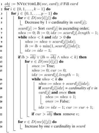
We now introduce the propagator. The principle is to tem-porarily reduce the domain of vector variables to each single value and update the lower-bound of Algorithm 1 on the fly, in order to determine whether this value should be removed or not, given the current upper-bound of obj domain. Al-gorithm 2 applies this idea while keeping a reasonable time complexity. Given any variable x, x and x are the minimum and maximum value in its domain D(x). After simulating that a domain is emptied, to compute the lower bound inde-pendently from the current variable, the algorithm checks if

the assignment of each value v would lead to a number of dis-tinct vectors strictly greater than obj . In this case value v is removed. As removed values do not participate to the initial bound computation, removals do not change the lower-bound. It is sufficient to run the filtering algorithm once at each call of the propagator. Algorithm 2 uses the two global data scard and vec, as well as the objective variable obj .

We point out that Property 2 is valid for any algorithm based on a maximum independent set of G, including the lower bound obtained using the exact (and NP-Hard) com-putation. Therefore, theoretically, our propagator can be complementary to any approach based on the compatibility graph that might be derived from AtMostNValue propaga-tors [Bessi`ere et al., 2006; Cambazard and Fages, 2015]. Property 3 (Time complexity). LetP

Di be the sum of

do-mains sizes of the k × p variables in the vectors matrix. P

Di ≤ k × p × d, where d is the maximum domain size.

Algorithm 2 runs inO(max(P

Di×k, p × r)) time.

Proof. (Sketch) Algorithm 1 computes all cardinalities in O(max(P

Di, p × r)) by traversing domains, in each row

ccard [j]. In card [j], the minimum cardinality is 0 and the maximum one is k. A linear sort of card [j] can be performed using an array of size k + 1. As each domain contains at least one value, the sum of domain sizes in scard [j] is greater than or equal to k. The whole matrix scard can be sorted in O(max(P

Di, p × r)). Algorithm 2 calls Algorithm 1

once and then loops on all variable domains. If lb > obj (or nbco < k) then each value is assessed and the while loop (line 16) can have an order of magnitude of k, giving a worst-case result of O(P

Di×k). Other statements are dominated.

Experimental Assessment of Algorithm 2. We benched our propagator independently from the PCP, using Choco 3.3.3 [Prud’homme et al., 2014] on a I7-4720HQ linux lap-top with 16GB of RAM. Minimizing the objective of a single AtMostNVector constraint is a NP-Hard problem [Chabert et al., 2009]. We compared the number of nodes and time re-quired to find an optimal solution and to prove optimality on randomly generated domains, using a bottom-up scheme. We used a search strategy that does not require a random pro-cess: select the variable with the largest domain and split this domain at each choice point2_{. We generated series of 100}

instances with 24 variables and domains of 10/15/20 values, randomly generated from shuffled arrays of 20/30/40 values. We compared two propagators: (IS), a propagator based on the state-of-the-art lower bound (maximum independent set), where values are filtered similarly to Algorithm 2 but using the Favaron’s approximation instead of Algorithm 1; (ISC), the IS propagator used in combination with Algorithm 2.

Table 1 provides the number of instances where the opti-mal solution is proved in less than 5 minutes. Average time is computed with instances that are both solved by the two tech-niques. Average nodes are computed on all solved instances. The average number of nodes is reduced using ISC. A few instances are solved using ISC and not using IS.

2

Results are similar using a lexicographic order of variables. The instances are harder to solve and ISC always leads to less nodes.

Nb. Domain Number of Average Average

variables size: range Optimal proofs Nodes Time (sec.)

24 (6×4) 10: [0,19] 99 / 100 111840 / 13769 0.92 / 0.53 24 (8×3) 10: [0,19] 100 / 100 93468 / 72560 13.9 / 10.91 24 (6×4) 10: [0,29] 93 / 94 1555719 / 77518 7.67 / 2.9 24 (8×3) 10: [0,29] 100 / 100 217880 / 99161 16.36 / 11.8 24 (6×4) 15: [0,39] 100 / 100 1074183 / 70814 11.39 / 7.65 24 (6×4) 20: [0,39] 99 / 100 636983 / 16450 3.6 / 1.23

Table 1:IS / ISC. Results on 100 instances, 5 min. time limit.

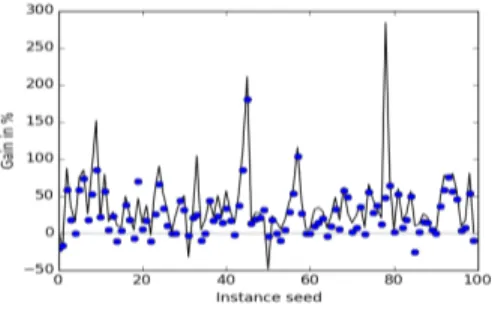
Figure 2:Gain and loss in nodes and time using ISC. The graph represents gain/loss in number of nodes for each of the 100 in-stances. Dots represent the gain/loss in time per instance.

Figure 2 shows gain and loss in % when ISC is used, in comparison with IS. The black graph represents gain/loss in number of nodes of each of the 100 instances for the data set where we observed the lowest benefit using ISC, 24 variables (8×3) with domains generated from a range of 20 values. Dots represent the gain/loss in time per instance. Figure 2 shows that ISC is the more robust technique. Almost all in-stances with a loss are easy. The maximum loss in time using ISC (-25%) occurs for an instance (85) that is solved in less than 0.04 sec., which has not a lot of meaning in Java.

In a last experiment, we computed average time for a first solution on 100 backtrack-free instances, in order to check Algorithm 2 scalability, using Choco 3. Results are 75.1 sec. for 10000 variables (2500×4) and 10 values per domain and 40.7 sec. for 100 variables and 1000000 values per domain.

4

Experimental results on PCP instances

We solved three real instances of the PCP in the field of gene therapy for retinal blinding diseases. The first one is related to the development of a gene addition therapy [Boye et al., 2012] in three animal models of inherited photorecep-tor dystrophies: a dog model of PDE6 β-retinitis pigmentosa, a dog model of RPGRIP1 -leber congenital amaurosis and a rat model of RDH12 -retinitis pigmentosa. In each model, one dog/rat sequence as well as one human sequence gene are evaluated. The problem considers the cloning of six in-serts (number of candidate sites between 31 and 56), with the use of six intermediate plasmids (number of candidate sites between 14 and 16). The second one is related to the de-velopment of a neuro-protective strategy to delay cone pho-torecetor degeneration in a mouse model of retinitis pigmen-tosa [Punzo et al., 2012]: 6 inserts (39 to 54 sites) and 3 intermediate plasmids (18 to 20 sites). The third one refers to an optogenetic therapy to restore visual perception at late stages of retinal degeneration [Sahel and Roska, 2013]: 7

in-serts (47 to 56 sites) and 2 intermediate plasmids (3 and 14 sites). Table constraints involve up to millions of tuples. We used the solving scheme described in section 3.1, with LastK-Conflicts [Lecoutre et al., 2009]. This “meta-mechanism” allows to guide search toward sources of conflicts. Using LastKConflicts, the best variable strategy was to assign first the final plasmid vars, and then the remaining vars for each insert successively, and then the costs, simply using the lexi-cographic order within each subset, with minimum value se-lection. The LastKConflicts best parameter is 2, probably be-cause the model is strongly structured along variable pairs.

Inst. Nb. P _{Opt. Opt. Nodes Time}

vect. costs vect. cost. (sec.)

Full1 1 24 yes yes 205 / 188 2.4 / 2.3

2 24 - yes 905 / 723 2.6 / 2.3

Real1 1 24 yes yes 66 / 66 1.4 / 1.4

2 24 - yes 97 / 84 0.8 / 0.8

Simu1 4 38 yes yes 2.1K / 2.1K 5 / 4.5

5 35 - yes 10.6K / 10.6K 7 / 7.2

Full2 1 24 yes yes 100 / 100 2.8 / 2.8

2 24 - yes 3.3K / 3.1K 8.6 / 8.3

Real2 3 35 yes yes 30.7K / 21.4K 33.9 / 26.1

4 26 - yes 42.5K / 39K 29.5 / 29.3

Simu2 4 24 yes yes 34.8K / 21.1K 24.6 / 17.3

5 24 - yes 4.7K / 4.6K 3.1 / 3.1

Full3 1 44 yes yes 293 / 293 4.2 / 4.2

2 35 - yes 4.2K / 3.4K 8.9 / 6.9

Real3 2 38 yes yes 508 / 508 4.6 / 4.7

3 33 - yes 6.5K / 5.7K 9.5 / 8.1

Simu3 3 37 yes yes 955 / 937 6.3 / 6.2

4 33 - yes 3.3K / 3.3.K 5.7 / 6.2

Table 2: IS / ISC. Results on full, real and simulated instances. Instance, number of vectors, sum of costs, proof of optimality for vectors and costs, nodes and time. Size of instances: 1 and 2: 141 variables, 80 constraints. 3: 164 variables, 96 constraints. Proof of optimality of cost sum is considered given the current value of the number of vectors (2 Pareto points: the second row corresponds to the best cost result when the number of vectors is relaxed by 1).

Table 2 shows the results, following the solving scheme presented in Section 3.1. Fulli are the three real instances

considered in a perfect world where all existing enzymes are available in the laboratory. Reali are the same instances but

with enzymes available in collaborator’s laboratory. Simui

are instances derived from Realiby randomly modifying 30%

of enzymes in components. The time limit was 5 minutes for each minimization step. LastKConflicts turned out to be of major importance in the solving process. All solutions were proved to be optimal for the two points of the Pareto front that make sense in practice. The results demonstrate the rel-evance of our constraint model for solving real instances of the PCP. They confirm a gain of solving robustness when AtMostNVector is propagated using Algorithm 2 (ISC), al-though this gain is mitigated by the use of LastKConflicts.

5

Conclusion

We provided a solution technique to the Plasmid Cloning Problem (PCP) in molecular biology. Our approach optimally solved real instances in the domain of gene therapy for retinal diseases. In addition, from a generic point of view in Con-straint Programming, we proposed a new propagator for the AtMostNVector constraint, proved to be complementary to the existing ones. Future work includes the development of a user-friendly software product for biologists, based on the proof of concept offered by this research work.

References

[ApE, 2015] ApE. ApE, a plasmid editor. http: //biologylabs.utah.edu/jorgensen/

wayned/ape/, 2015.

[Appleton et al., 2014] Evan Appleton, Jenhan Tao, Traci Haddock, and Douglas Densmore. Interactive assem-bly algorithms for molecular cloning. Nature Methods, 11(6):657–662, 2014.

[Backeman, 2013] Peter Backeman. Propagating the nvector constraint : Haplotype inference using constraint program-ming. Technical Report IT, 13 056, URN:diva-211862, Uppsala University, Master dissertation, supervised by Pierre Flener, East Lansing, Michigan, 2013.

[Bessi`ere et al., 2006] Christian Bessi`ere, Emmanuel He-brard, Brahim Hnich, Zeynep Kiziltan, and Toby Walsh. Filtering algorithms for the NValue constraint. Con-straints, 11(4):271–293, 2006.

[Biolabs, 2015a] New England Biolabs. Compatible en-zymes. https://goo.gl/hLfWEK, 2015.

[Biolabs, 2015b] New England Biolabs. Enzyme properties. https://goo.gl/7xVD8f, 2015.

[Biolabs, 2015c] New England Biolabs. Restriction en-donucleases. https://www.neb.com/products/ restriction-endonucleases, 2015.

[Boye et al., 2012] Shannon Boye, Sanford Boye, Alfred Lewin, and William Hauswirth. A comprehensive review of retinal gene therapy. Molecular therapy, 21(3):509– 519, 2012.

[Brown, 2010] Terence A. Brown. Gene Cloning and DNA Analysis: An Introduction. Wiley-Blackwell, 2010. [Cambazard and Fages, 2015] Hadrien Cambazard and

Jean-Guillaume Fages. New filtering for atmostnvalue and its weighted variant: A lagrangian approach. Constraints, 20(3):362–380, 2015.

[Casini et al., 2015] Arturo Casini, Marko Storch, Geoffrey Baldwin, and Tom Ellis. Bricks and blueprints: methods and standards for dna assembly. Nature reviews. Molecu-lar cell biology, 16(9):568–576, 2015.

[Chabert et al., 2009] Gilles Chabert, Luc Jaulin, and Xavier Lorca. A constraint on the number of distinct vectors with application to localization. In Ian P. Gent, editor, Proceed-ings CP 2009, volume 5732 of Lecture Notes in Computer Science, pages 196–210. Springer, 2009.

[Densmore et al., 2010] Douglas Densmore, Timothy Hsiau, Joshua Kittleson, Will DeLoache, Christopher Batten4, and J. Christopher Anderson. Algorithms for automated dna assembly. Nuclear Acids Research, 38(8):2607–2616, 2010.

[Favaron et al., 1993] Odile Favaron, Maryvonne Mah´eo, and Jean-Franc¸ois Sacl´e. Some eigenvalue properties in graphs (conjectures of graffiti - II). Discrete Mathematics, 111(1-3):197–220, 1993.

[Grac¸a et al., 2009] Ana Grac¸a, Jo˜ao Marques-Silva, Inˆes Lynce, and Arlindo L. Oliveira. Haplotype inference with

pseudo-boolean optimization. Annals of Operations Re-search, 184(1):137–162, 2009.

[Lecoutre et al., 2009] Christophe Lecoutre, Lakhdar Sais, S´ebastien Tabary, and Vincent Vidal. Reasoning from last conflict(s) in constraint programming. Artif. Intell., 173(18):1592–1614, 2009.

[Lecoutre et al., 2015] Christophe Lecoutre, Chavalit Likit-vivatanavong, and Roland H. C. Yap. STR3: A path-optimal filtering algorithm for table constraints. Artif. In-tell., 220:1–27, 2015.

[Mairy et al., 2014] Jean-Baptiste Mairy, Pascal Van Hen-tenryck, and Yves Deville. Optimal and efficient filtering algorithms for table constraints. Constraints, 19(1):77– 120, 2014.

[Perez and R´egin, 2014] Guillaume Perez and Jean-Charles R´egin. Improving GAC-4 for table and MDD constraints. In Barry OSullivan, editor, Proceedings CP 2014, volume 8656 of Lecture Notes in Computer Science, pages 606– 621, 2014.

[Prud’homme et al., 2014] Charles Prud’homme, Jean-Guillaume Fages, and Xavier Lorca. Choco3 Documen-tation. TASC, INRIA Rennes, LINA CNRS UMR 6241, COSLING S.A.S., 2014.

[Punzo et al., 2012] Claudio Punzo, Wenjun Xiong, and Connie Cepko. Loss of daylight vision in retinal degen-eration: are oxidative stress and metabolic dysregulation to blame? Journal of Biological Chemestry, 287(3):1642– 1648, 2012.

[Sahel and Roska, 2013] Jose-Alain Sahel and Botond Roska. Gene therapy for blindness. Annual Review of Neuroscience, 36:467–488, 2013.