HAL Id: hal-03137239
https://hal.archives-ouvertes.fr/hal-03137239
Submitted on 6 May 2021
HAL is a multi-disciplinary open access
archive for the deposit and dissemination of
sci-entific research documents, whether they are
pub-lished or not. The documents may come from
teaching and research institutions in France or
abroad, or from public or private research centers.
L’archive ouverte pluridisciplinaire HAL, est
destinée au dépôt et à la diffusion de documents
scientifiques de niveau recherche, publiés ou non,
émanant des établissements d’enseignement et de
recherche français ou étrangers, des laboratoires
publics ou privés.
Distributed under a Creative Commons Attribution| 4.0 International License
the Ligurian current (northwestern Mediterranean)
using a bio-optical glider
Katarzyna Niewiadomska, Hervé Claustre, Louis Prieur, Fabrizio d’Ortenzio
To cite this version:
Katarzyna Niewiadomska, Hervé Claustre, Louis Prieur, Fabrizio d’Ortenzio. Submesoscale
physical-biogeochemical coupling across the Ligurian current (northwestern Mediterranean) using a bio-optical
glider. Limnology and Oceanography Bulletin, American Society of Limnology and Oceanography,
2008, 53 (5part2), pp.2210-2225. �10.4319/lo.2008.53.5_part_2.2210�. �hal-03137239�
Submesoscale physical-biogeochemical coupling across the Ligurian Current
(northwestern Mediterranean) using a bio-optical glider
Katarzyna Niewiadomska, Herve´ Claustre, Louis Prieur, and Fabrizio d’Ortenzio
CNRS, UMR 7093, Laboratoire d’Oce´anographie de Villefranche, 06230 Villefranche-sur-Mer, France; Universite´ Pierre et Marie Curie-Paris 6, UMR 7093, Laboratoire d’Oce´anographie de Villefranche, 06230 Villefranche-sur-Mer, France
Abstract
A bio-optical autonomous underwater gliding vehicle, equipped with a conductivity, temperature, depth (CTD) sensor, an oxygen sensor, backscatter meters, chromophoric dissolved organic matter (CDOM) and chlorophyll fluorometers, and upwelling and downwelling radiometers was developed to characterize the biogeochemical response to physical forcing at the submesoscale (1–10 km). Winter data obtained in the northwestern Mediterranean basin in a 50-km transect that crossed the permanent, along-coast Ligurian Current show tight physical-biogeochemical coupling across the Ligurian Current, not observed using other sampling strategies. At the scale of the transect, the various biogeochemical parameters displayed independent behaviors, while at the submesoscale, there was a coherent covariance of these variables, especially in the frontal zone. Near-isopycnal tongues of elevated fluorescence and oxygen concentration were recorded down to a depth of 180 m and are the likely signature of a converging horizontal and downwelled water flow. Local anomalies in a horizontal section well below the mixed-layer depth are likely representative of downwelled waters from the euphotic layer. Intrusions of elevated CDOM concentrations together with signatures of smaller particles are the likely features of a local divergence and upwelled waters from subjacent aphotic layers. These are particularly apparent in the form of local anomalies in a horizontal section within the mixed layer. Similar tongues were observed in data from subsequent glider deployments. Such biogeochemical signatures enable the identification of upward and downward physical motions not observed by other technologies, reinforcing the need for coupled high-resolution physical-biogeochemical studies, not only for investigating biogeochemical processes themselves but also for resolving physical processes at these scales.
In the ocean, mesoscale (10–100 km) and submesoscale (1–10 km) processes have a strong effect on large-scale circulation and local redistribution of heat and salt. Via the turbulent diffusion mechanism, they modify the actual temperature and salinity fields, induce oceanic mixing, and provoke horizontal and vertical motion (Van Haren et al. 2004). They also play an important role in the redistribu-tion of chemical elements at large scales (e.g., basin scale), influencing then the structure and the spatio-temporal organization of marine biomass (Wunsch and Ferrari 2004). Moreover, at submesoscales where ageostrophic flows may induce high vertical velocities, physical forcing triggers biological and subsequently biogeochemical re-sponses. This occurs essentially because time scales of
upward motions could match time scales of biological ones (e.g., phytoplankton growth) (Zakardjian and Prieur 1998).
Our perception of this biophysical coupling at subme-soscales nevertheless relies mostly on numerical experi-ments (Franks 1992; Nurser and Zhang 2000; Levy et al. 2001). However, for modeling exercises to be informative, they must be continuously constrained by observations collected at the appropriate temporal and spatial scales. To reveal and understand such submesoscale biophysical coupling, the observational strategies must associate a high spatial resolution with a multivariable approach that enables the physical, chemical, and biological fields to be simultaneously documented.
Presently, such types of observations (e.g., using Seasoar or Towyo) are scarce because of the difficulty in designing appropriate sampling strategies from ship-based platforms (Pinot et al. 1995; Yanagi et al. 1996) and the high cost of their implementation. The permanent front associated with the jet of modified Atlantic waters that flows in the Mediterranean Alboran Sea near the Straits of Gibraltar, the so-called Almeria–Oran front, is a good example of where such strategies have been applied on dedicated cruises (ALMOFRONT, OMEGA) and have led to unparalleled observations (Fasham et al. 1985; Prieur and Sournia 1994; Allen et al. 2001). Nevertheless, these remain costly and are likely unadapted if the variability of the biophysical coupling must be studied at specific time scales (e.g., seasonal scale or event scale [effect of winds]) or if the occurrence of such structures must be monitored at larger scales (e.g., basin).
Acknowledgments
We thank A. Poteau, D. Taillez, and P. Senotier for their technical support during glider operations, and G. Be´cu and the captain and crew of the R/V Te´thys II for their cooperative work at sea. We gratefully acknowledge A. Mangin and ACRI for continuously providing weather-related forecasts and hindcasts.
This is the contribution of the TOSCA/CNES/PROGLO (Terre Ocean Surface Continental Atmosphere/Centre Nationale des E´ tudes Spatiales/PROfileurs et GLiders Optiques) program, with additional support from the French ANR-PABO (Agence Nationale de la Recherche–Platformes Autonomes et Biogeochi-mique Oceanique) program and KORDI (Korea Ocean Research and Development Institute). Contribution by the Poˆle de competitivite´ mer-Provence-Alpes-Coˆte-D’azur is also acknowl-edged. The Boussole project was an indispensable part of this work and all contributors are much appreciated.
New observational strategies must therefore be imple-mented. Autonomous underwater gliders are beginning to prove their large potential in the high-resolution descrip-tion of hydrologic (temperature, salinity) fields (Rudnick et al. 2004; Schofield 2007). These new platforms point to an extremely promising path, leading to unprecedented investigations in the study of biophysical coupling and, more generally, of oceanic biogeochemistry for several reasons. First, they operate over a scale continuum ranging from the submesoscale to the basin scale (1–1,000 km). In comparison to classical strategies that make use of research vessels, this is an essential characteristic of these platforms, particularly in investigating the issues of scale transfer, the effect of small scales on larger ones and vice versa (e.g., Levy 2003). Second, new generations of miniaturized, low-energy, chemical, optical, and biological sensors are being (and will continue to be) developed. Implemented on these new platforms, they enable repeated high-resolution observations of physical forcing and associated biogeo-chemical responses. Finally, continuous and simultaneous observations of physical and biological parameters ob-tained from a biogeochemical glider offer the possibility of implementing innovative approaches to deriving informa-tion on ocean hydrodynamic processes. Certain biogeo-chemical variables (e.g., oxygen) are already considered as tracers of dynamic (physical) processes and are subsequent-ly used to derive additional information on the circulation of water masses (e.g., Broecker 1974; Broecker et al. 1985). With a glider, a similar approach could be extensively applied, particularly in exploring temporal and spatial scales that were very poorly examined up to now.
We have developed a bio-optical glider (nicknamed Tournesol) to monitor biogeochemical properties (chloro-phyll a [Chl a]), particle load and size, colored dissolved organic material [CDOM], and oxygen concentration) with the same resolution as hydrological properties (tempera-ture, salinity). For the first time, a glider is used as a dedicated platform to study biophysical coupling on a permanent jet-front system.
In the open ocean, a frontal-jet system is composed of a frontal structure, associated horizontal density gradients, and geostrophic currents. These jets are not in strict geostrophic balance so that submesoscale agesotrophic circulation takes place involving vertical velocities, conver-gences, and divergences (Fedorov 1986). Such systems are known to enhance biological production when time scales of vertical ageostrophic velocities and the associated input of nutrients in well-lit layers are compatible with the time scales of production processes (Williams and Follows 2003). Many physical processes could explain the enhance-ment of vertical velocities (on the order of (O) 1–80 m d21)
near fronts such as baroclinic instabilities (Levy 2003) and turbulent flux-induced instabilities (Thomas and Lee 2005; Giordani et al. 2006). Such vertical velocities resulting in ageostrophic secondary circulation remain difficult to measure. Indeed the influence of secondary circulation in stimulating primary production is known as a ubiquitous feature (Sournia et al. 1990; Claustre et al. 1994b; Allen et al. 2005), and such stimulation is often sufficiently recurrent to sustain higher trophic levels (Boucher et al.
1987; Fielding et al. 2001). It follows that the analysis of the biological and chemical signatures could then be used to (1) identify the location of these structures and (2) improve the interpretation of the purely physical observations.
In this article, we have taken the case study of the geostrophic Ligurian frontal jet flow (northwestern Med-iterranean), a permanent structure (Sournia et al. 1990) resulting from the cyclonic circulation of the Northern Current (Millot 1999) that flows generally along the Ligurian, Provencal, and Catalan coasts, despite occurring meanders, in a band ,30 km wide and to a depth of .250 m. Flowing jet waters near the surface separate the area into light coastal waters (marginal zone) and an open-water zone (central zone) with elevated surface densities (Prieur 1979). The geostrophic front lies also at depth as a strong horizontal density gradient. The interface between the marginal zone and the central zone, i.e., the frontal zone, is the site of various multi-scale and little-known interactions between physical, biological, and chemical processes that locally enhance biological production and could be the result of submesoscale processes. A vertical circulation scheme linked to the Ligurian Current front was developed in detail by Boucher et al. (1987) on the basis of in-situ hydrographic and biological observations. In this conceptual scheme of the vertical circulation, a set of alternating divergences and convergences exist in the space of about 70 km from the marginal zone outward into the central zone.
As part of the present study, our central objective is to interpret high-resolution, cross-jet observations made by a bio-optical glider and to resolve the biogeochemical responses to the physical forcing at submesoscales. In particular, we evaluate how biogeochemical properties might enable the identification of submesoscale structures resulting from ageostrophic secondary circulation. These measurements are interpreted in the context of a more comprehensive set of observations, including simultaneous Acoustic Doppler Current Profiler (ADCP) data. Regional-scale remote sensing is used to give a more global context of the deployment zone. The particulate matter composition is additionally discussed, and the possible permanence or recurrence of the observed submesoscale structures at other periods of the year is investigated through a brief description of subsequent transects.
Materials and methods
Bio-optical glider and integrated sensors—The Slocum electric gliders are buoyancy-controlled self-propelled underwater vehicles developed by Webb Research Corpo-ration. By changing their buoyancy, gliders advance through the water column in a vertical gliding saw-tooth pattern, coming periodically to the surface for GPS repositioning and data transmission. The bio-optical glider developed for our purposes (Fig. 1) is capable of diving to a depth of 1,000 m and carries fluorometers, radiometers, backscatter meters, an oxygen sensor, and a conductivity, temperature, depth (CTD) sensor. Although some of these sensors have been used independently in gliders before, to the authors’ knowledge this is the first glider carrying such
a comprehensive set of optical and biogeochemical sensors that is dedicated to biogeochemical investigations.
The CTD onboard the glider is a non-pumped, low-drag, continuous-profile Sea-bird CTD (SBE-41). Wetlabs pro-vides a combination backscatter meter and fluorometer (BB2FLS ECO puck) that measures single-angle backscat-tering at two wavelengths and a single excitation and emission fluorescence response. Two of these sensors were integrated into the biogeochemical glider, resulting in four measurements of backscatter and two fluorescence re-sponses. Backscatter is measured at wavelengths of 880 nm, 660 nm, 532 nm, and 470 nm at a backscatter angle of 117u. CDOM fluorescence is excited at 370 nm for emission at 460 nm, whereas Chl a fluorescence is excited at 470 nm for emission at 695 nm. The OCR-504I/R sensors by Satlantic were designed specifically to match the diameter of the Wetlabs sensors for modular integration into existing Slocum glider payloads. The OCR504I is upward looking, angled at 220u to the horizontal plane for data sampling on the upcast only and measures downwelling irradiance (Ed) at
412 nm, 443 nm, 490 nm, and 555 nm. The OCR504R is downward looking, angled at+20u to the horizontal plane for data sampling on the upcast only and measures upwelling radiance (Lu) at the Ed wavelengths. The
Aanderaa oxygen Optode 3830 is a standard off-the-shelf sensor used to measure oxygen concentration. This sensor is configured to output factory-calibrated engineering units: the differential phase shift (d-phase) information. Because of space constraints in the sensor payload, this sensor is placed in the rear of the glider but the optical window has an unobstructed field-of-view into the surrounding water.
Deployment—The glider mission began at 13:25 h on 28 Jan 2007 at the point VF (Villefranche) off the coast of Nice, France (Fig. 2), in an area where the margin is very steep and nearshore waters exceed 500 m within 0.5 km of the coast. The glider was deployed at ,1 km distance from the nearest landmass (Cap Ferrat), performing yos (1 yo 5 1 dive and 1 climb) in a 10–500-m layer with a surface interval of 4 hours (;2 yos) for data transmission and GPS
positioning. The glider transect traverses the Northern Current (the Ligurian Sea section) in a southeast offshore direction (Fig. 2) and ends at the point DF (Boussole-DYFAMED: http://www.obs-vlfr.fr/Boussole/html/project/ boussole.php), a permanent time series sampling site where an optics buoy is anchored (43u259N, 7u529E). The glider was recovered at 10:00 h on 31 Jan 2007 at the point DF. Total mission time was ,68.5 h, including data transmis-sion and surface drift time, covering an effective distance of 48.5 km.
Monthly glider deployments are planned to coincide with monthly ship-based missions (R/V Tethys II) to the point DF. The current field along the transect is retrieved from the shipboard ADCP of the R/V Tethys II, and discrete measurements made at the mooring are used for validation and calibration purposes.
Meteorological conditions—Air temperatures before de-ployment ranged from 5uC to 7uC and rapidly increased to 11uC during the first 2 days of deployment. This temperature was maintained throughout the remainder of the transect. Winds were primarily southwest 2 days before deployment with speeds of 4–6 m s21 and northeast with
speeds of 2 m s211 day before deployment. On the day of
deployment wind speeds were close to zero, and a southwesterly wind averaged 5 m s21for the 3 ensuing days.
Data processing—Geolocation: Because actual GPS positions are taken only every 4 hours (at surfacing), they are interpolated to provide a GPS position for every data point in the data set (1 point every 2 seconds). These positions are then projected along a straight line running from the coastal deployment point (VF) to the offshore destination point (DF). A projection parallel to the coastline is used making a 236u angle with the VF–DF line. This direction corresponds to the azimuth angle of the depth-averaged Northern Current as seen in Fig. 2. Some gaps in the data are observed because of operational difficulties, and these gaps are not interpolated. The distance travelled is subsequently calculated using the
Fig. 1. Glider Tournesol and the associated sensors: (a) Seabird CTD cell (S,T); (b) Wetlabs BB2FLS (bbp(660, 880 nm) and CDOM); (c) Satlantic OCR504I Radiometer (Ed); (d) Aanderaa
3830 optode (O2); (e) Wetlabs BB2FLS (bbp(470, 532) and Chl a); (f) Satlantic OCR504R
deployment point VF as distance zero. This procedure is performed primarily to permit inter-comparison of month-ly transects and for comparison with ADCP data.
Raw data: The oxygen sensor is configured to output d-phase information (resolution ,1 mmol L21, accuracy
5%), which is used in conjunction with the CTD temperature output to derive oxygen concentration [O2]
according to calculations in the Aanderaa manual (www. aadi.no). Because the CTD is non-pumped, thermal lag effects leading to significant salinity bias as a result of heat stored in the conductivity cell walls can occur. This is typically seen when a temperature gradient .0.2uC m21
exists between surface and deeper waters (which is not the case here). Simple lag and time-constant corrections based on the work of Morison (1994) and extended by Kerfoot (unpubl.) were applied to the glider CTD data in order to avoid salinity and oxygen bias. Salinity (S), potential temperature (h), and potential density (s) are calculated based on corrected conductivity, corrected temperature (T ), and pressure from the glider CTD using the Unesco polynomial (Fofonoff and Millard 1983). The backscatter meters (sensitivity ,O(1025) m21sr21) output a
factory-calibrated volume scattering coefficient b(117u, l) which is then used to calculate the particulate backscatter bbp(l)
m21 as described in the Wetlabs ECOBB2FLS Manual
(www.wetlabs.com). The fluorometers are also factory calibrated, outputting Chl a concentration [Chl a]
(sensi-tivity 0.01 mg m23) and CDOM concentration [CDOM]
(sensitivity 0.25 relative units [rel. units]) values.
Once the glider Tournesol is retrieved at point DF, it is strapped vertically onto the R/V Tethys II ship-board CTD rosette for cross-calibration, and both are lowered at a speed matching the average net displacement speed of the glider. Glider CTD and [O2] measurements are validated
against ship-based Seabird CTD and O2 sensors, but no
corrections are made. [Chl a] measurements are post-calibrated against the CTD rosette fluorometer, which is calibrated against high performance liquid chromatogra-phy (HPLC) samples. It should be noted that [CDOM] and bbpare only factory calibrated, but this does not present an
issue as it is the relative differences that we are mainly concerned with here.
After conductivity and temperature lag-corrections (see above), glider salinity and temperature matched the ship-based CTD values to within 2%. Glider [O2] calculated
using T yielded results within 7% of shipboard [O2] values,
resulting in a possible bias on the order of ,25 mmol L21.
CDOM concentration in the oligotrophic Mediterranean is typically very low. In our case, measured [CDOM] ranged from 3 to 4 rel. units. However, enough variability remains to enable observation of the features present.
The spectral dependence of the backscattering coefficient is described by its spectral slope c, and is approximated as bbp(l) , Cl2c (where C is a constant). Thus, c is simply
calculated as the slope of the linear regression between
Fig. 2. Map of deployment zone in the northwest Mediterranean. Glider transect (projected onto black line) starting on 28 Jan 2007 off the coast of Nice, France (VF, triangle) and ending on 31 Jan 2007 at the Boussole/DYFAMED site (DF, circle). Gaps represent surface drift time and interruptions due to logistical issues. MF is the point between the marginal and frontal zones and FC the point between the frontal and central zones. Inset: Mediterranean Sea showing the glider deployment area. (Ocean Data View [ODV] Software, version 3.2.2, R. Schlitzer; http://odv.awi. de/).
log(l) and log(bbp(l)) using l 5 550 and 880 nm only.
Based on theoretical studies and in-situ studies (e.g., Reynolds et al. 2001; Stramska et al. 2003), c has been proposed as an index characterizing the slope of the particle size distribution for particles lower than 10 mm (Loisel et al. 2006). The higher the c (the steeper the slope), the higher the contribution of small particles over total number of particles, and reciprocally. Backscatter spectral slope c is relatively insensitive to the refractive index variations (Stramski et al. 2001). Some flattening in the bbpspectrum
(resulting in a lower c) is possible under conditions of strong blue absorption (CDOM, pigments). This effect can be disregarded because only the green and infrared wavelengths were used for calculating c in this article.
The depth of the euphotic layer, defined as the depth where irradiance is reduced to 1% of its surface value, was based on [Chl a] profiles using the relationship proposed by Morel and Berthon (1989) and extended by Morel and Maritonera (2001). The mixed layer depth (MLD) was calculated as the depth at which the potential density is equal to the potential density at 10 m plus 0.005 kg m23 (MLD 5 Depth(d
10m + 0.005) m).
Tourne-sol’s radiometric measurements Ed(l) and Lu(l) were not
used in this article.
The entire transect yields 64 individual casts to 500 m each. Because little biogeochemical variability is seen at depth, we have chosen to limit the shown data to the surface 250-m layer for better observation of small-scale features. In this article, data shown are interpolated for clarity; however, all results, calculations, and interpreta-tions are based on non-interpolated data. Interpolation of variables on the line VF-DF was performed using a standard Ocean Data View (ODV Software, version 3.2.2, R. Schlitzer; http://odv.awi.de/) VG gridding procedure where a variable resolution, rectangular grid with x and y grid spacing varies according to data density. Property values at every grid point are calculated using a simple weighted-averaging scheme.
ADCP currents: Processed data from the R/V Tethys II ADCP (RDI VM BB150 KHz) were obtained from the INSUDT (Institut National des Sciences de l’Univers -Division Technique) data service center (http://saved.dt. insu.cnrs.fr/). Standard data processing for angle and magnitude corrections (Pollard and Read 1989) requires heading measurements made by a double-antenna GPS, which was malfunctioning for the days in question. Ship heading was therefore supplied by an onboard Gyrocom-pass, and the GPS position was supplied by the shipboard GPS. ADCP data were therefore additionally processed for angle (1.0u) and magnitude (0.9987) corrections, taking into account the velocity angle difference between the ADCP (Vwater) and ship (Vgps) referentials by the method of minimum correlation between Vwater and Vgps. This method yields an angular precision of 0.1u, leading to a Vwater precision in absolute value on the order of 1 cm s21. Corrected, averaged data (43 pings min21) were
filtered to keep bins containing Verror values inferior to 5 cm s21, using filters designed to eliminate infrequent
spiking associated with poor sea conditions and to lower
the noise of calculated velocities under 1 cm s21,
respec-tively. The data shown herein are a coast-to-open-water transect dating 30 Jan 2007, corresponding to the same day Tournesol traversed the current.
Satellite data: Satellite MODIS-AQUA high-resolution level-2 images (http://oceancolour.gsfc.nasa.gov/) were pro-cessed using SEADAS software (version 5.1.4). The level-two files were remapped on an equirectangular projection, with [Chl a] and sea surface temperature (SST) products derived using NASA standard processing algorithms (Esaias et al. 1998). Only land and cloud L2 flags were applied on the ocean color images; therefore, obtained values of [Chl a] could be affected by an important error, particularly in the pixels closest to the coastline (i.e., case two waters). As our interest lies in the spatial patterns rather than the absolute values, we opted to keep ocean color images without applying all flags in order to maximize the number of observations in the area. Unfortunately, during the glider deployment, only the day of 30 Jan 2007 was cloud-free. Figure 3 shows the chlorophyll concentration distribution and the SST of the area for this day.
Results
Ancillary data—The main feature observed in the SST image (Fig. 3a) is the abrupt gradient (about 1uC) between the coastal (warmer) and the offshore (colder) regions, a well-known characteristic of the area in winter (Sournia et al. 1990). Chl a concentration distribution (Fig. 3b) is similar to that of SST, although more patchy, and shows higher values in the offshore area along a line parallel to the coast at approximately 20–30 km. In the [Chl a] map, a filament of elevated surface biomass is evident inside the coastal and frontal zones at about 7.5u longitude. This structure, however, cannot be confirmed because of poor image resolution at such proximity to the coast and the quality of the raw data used. In additional images available only days later, this structure was not evident. No signature of this feature was detected either in the SST satellite data or on data from Tournesol (see Glider data), which crossed the position of the patch the previous day. This patch, if verified, would have actually been situated ,40 km to the northeast on 29 Jan 2007, the day the glider traversed that section. Note that in Fig. 3, the satellite images, the ADCP horizontal velocities in blue, and the portion of the glider trajectory shown in solid green are all data sampled on 30 Jan 2007. It can be hypothesized that this filament corresponds to a very rapidly moving structure. In other non-synoptic satellite images before and after deployment, the only coherent structure seen was the existence of the front, both in [Chl a] and in SST.
The averaged horizontal current flow (Fig. 4a) has a maximum value of 60 cm s21, an average direction of
,250u north, and drops below 10 cm s21 at 30 km
distance. Weak oscillations on the central side of the current (border fixed as surface velocity ,20 cm s21) were
observed without significant directional changes over 4 days.
The partitioning between the frontal and central zones is put into evidence by the gradient in temperature (Fig. 3b); however, the offshore limit of the ADCP current falls further beyond the temperature division. The weak oscillations of this temperature boundary parallel to the coast were evaluated as non-significant given that the current during this period did not exhibit pronounced meanders, thus excluding a strong cyclotrophic component to the jet.
Glider data—The region was divided into three distinct zones on the basis of the potential density field (s): the marginal (M) zone (coastal region), a frontal (F) zone that encompasses the jet-like current area, and the central (C)
zone (open water) beyond the front. The limit between the marginal zone and the frontal zone, MF (Fig. 2), was determined as the distance where the rapidly increasing slope of the 28.65–28.95 kg m23density layer offshore and
upwards occurs, and lies at ,15 km. Similarly, the limit FC between the frontal and central zones is determined using the rather sharp decreasing slope on the offshore side of the jet and lies at 30 km. Note that this definition of limits puts the jet with velocities .20 cm s21 inside the frontal zone
(Fig. 4a) and is coherent with the geostrophic thermal-wind equation that drives the primary horizontal circulation. Note also that the surface density front, which lies near 28 km, does not coincide exactly with FC. This fact will be discussed later. The same kind of delimitations were used previously in papers describing annual properties of water mass, large particles, and zooplankton (Boucher et al. 1987; Stemmann et al. 2007).
The marginal zone is characterized by a warm, light, surface layer (0–150 m) of Modified Atlantic Waters (MAW) (Millot 1999). Colder (13.2–14uC), more saline (38.5–38.7) Levantine Intermediate Waters showing double peaks on the h-S plot (Fig. 5) lie below 150-m depth.
In the central zone, a layer of cold surface water (0– 75 m), more saline than the marginal waters, sits atop heavier, warm, salty waters. A known phenomenon in this part of the Mediterranean is the occasional cooling of MAW at the surface due to cold gusts of northwesterly winds without any significant mixing. This specific water mass, called Winter Intermediate Water (WIW) by Salat and Font (1987), typically has temperatures below 12.4uC and salinities of ,38.3. A clear doming (particularly apparent at the 29 kg m23 isoline) at km 32 is observed
in all physical and biogeochemical properties, pushing the interface of these values surfaceward by ,25 m.
The frontal zone can be seen as a transition zone between the cold central-zone water properties and the warmer marginal-zone water properties (Fig. 4). The color distri-butions on each panel are coincident with the isopycnal lines; however, strong anomalies were observed mainly around the FC limit. A near-isopycnal tongue of cold surface water (13.25uC, 38.35) ,4 km wide is observed up to a depth of 180 m.
This anomaly in temperature and salinity seen in the frontal zone is also observed in [O2], [Chl a], [CDOM], and
less clearly in bbp (only bbp(470) is shown) with typical
surface values observed down to 180-m depths. A second tongue at km 18 (,5 km wide) can be seen in [Chl a] and [CDOM], but is less apparent in [O2]. This second feature is
not seen at all in S, h, s, bbp(470), and c. Elevated [CDOM]
values are observed on the marginal side of each tongue, correlating with reduced levels of particulate backscatter in the case of the larger tongue. The highest values of bbp(470)
are observed between km 24 and 26 in the upper 50-m layer, correlating with the high velocity values of the Northern Current and located at the surface boundary of the front. The spectral dependence c likewise shows the lowest values (high contribution of large particles over total particles) at the same location.
The highest particulate backscatter, bbp(470), and lowest
spectral dependence (c) values are found in the surface layer
Fig. 3. Satellite image for 30 Jan 2007, 12:00 h, for the glider deployment zone off the coast of Nice, France (northwest Mediterranean). The actual glider trajectory from the coast to the Boussole/DYFAMED site during 28–31 Jan 2007 deployment is shown in a solid black line. The part of the glider path corresponding to the day of the satellite image and to the ADCP data (30 Jan 2007) is superimposed in solid green. Gaps in the trajectory correspond to data transmission at the surface and other interruptions due to logistics. The glider path projection-line from VF to DF is shown in a red solid line. The blue lines (stick plot) represent ADCP horizontal velocities on 30 Jan 2007 (7:00 h to 12:00) averaged in the 20–150-m layer along the transect of R/V Thethys II to the Boussole/DYFAMED site. (a) MODIS-AQUA [Chl a] distribution; (b) MODIS-AQUA SST.
of the marginal zone but [Chl a] remains low (,0.25 mg m23) (Fig. 4f,h,i). Comparatively lower values
of bbp(470) and higher values of c (greater abundance of
smaller particles over total ones) are observed in the surface waters of the central zone, whereas [Chl a] is higher (up to
0.8 mg m23). Oxygen concentrations are homogeneous in
the entire surface layer, with high concentrations (230 mmol L21) reaching depths of 100 m in the marginal zone and
50–80 m in the central zone. Similarly, relatively low [CDOM] values are homogeneous across the surface layer,
Fig. 4. ADCP currents (30 Jan 2007) and glider hydrographic data (28–31 Jan 2007) with density isolines in black; horizontal white dotted lines show the depth sections used in Figs. 7 and 8. MF is the point between the marginal and frontal zones and FC the point between the frontal and central zones. White spaces indicate areas where no data was retrieved because of surface drift and logistical issues. (a) Transect of ADCP currents (repeated at the top of both figure columns); (b) glider potential density, vertical gray lines indicate real glider ‘‘yos’’ to show data resolution; (c) glider salinity; (d) glider potential temperature; (e) glider oxygen concentration; (f) glider chlorophyll concentration, the euphotic depth is shown in red and the MLD in heavy black; (g) glider CDOM concentration; (h) glider particulate backscatter at 470 nm; (i) glider backscatter spectral dependence c. (Ocean Data View [ODV] Software, version 3.2.2, R. Schlitzer; http://odv.awi.de/).
extending to 100-m depth in the marginal zone and up to 80 m in the central one. Additionally, surface patches of relatively higher [Chl a] are observed at kms 28, 35, and 49. Other anomalies, such as filamental structures in the ADCP currents (km 7), and weak fluctuations of surface density, salinity, and temperature in the marginal zone could be seen for some variables, but were not evidenced in the variable fields recorded by the glider. Such structures could be the result of wind effects and/or diurnal heating. As these processes are outside the scope of this article, they will not be further detailed here.
In summary, the front clearly delineates two different water masses: a warm, low [Chl a] coastal region and a colder, high [Chl a] open water region. There is coherence between the physical values and some biogeochemical parameters while others are uncorrelated. Two near-isopycnal tongues of surface water are observed primarily in temperature and biogeochemical parameters. Density doming is evident in the central zone, whereas values of [CDOM] decreasing from depth toward the surface are apparent on both sides of the front. In the following section, we provide an interpretation for the features observed, their significance, and their possible driving mechanisms.
Discussion
Vertical circulation scheme—Figure 6 represents a sche-matic of the biogeochemical field response to vertical velocities associated to a jet-front system. Consider a hypothetical simplified vertical advection model where a
horizontally homogeneous value of a variable V in a geostrophic flow (vertical velocities %1 m d21) is subjected
to a relatively large vertical water velocity w (e.g., w . 5 m d21) at a front (Fig. 6a). The velocity w is positive
between the isolines r 2hr and r and negative between the isolines r and r+hr. We assume the existence of two cases of initial conditions: the case where V has high concentra-tions at the surface and is decreasing with depth (case DWD; Fig. 6b) such thathV/hh , 0 (e.g., oxygen), and the case where V has low concentrations at the surface and is increasing with depth (case IWD; Fig. 6d), such thathV/hh .0 (e.g., CDOM). We take a horizontal section of V at a single depth and normalize these values. For the case DWD, where V is decreasing with depth, the deep waters having lower concentration values will flow upward along the isopycnals where w . 0 and the surface waters with elevated values will flow downward along the isopycnals where w , 0 (Fig. 6c). For the case IWD, where V is increasing with depth, the deep waters having higher variable values will flow upward along the isopycnals where w . 0 and the surface waters with reduced values flow downward along the isopycnals where w , 0 (Fig. 6e). This shift away from the initial conditions leads to the conclusion that local anomalies can give information on the orientation of vertical advection on a horizontal section, under the proviso that the water velocity w and the vertical advection of V are locally significant and that at least one other term in the conservation equation (e.g., horizontal advection) is significant enough to maintain equation equilibrium. Moreover, if the same anomaly were observed simultaneously throughout multiple variables, the presence of vertical advection would be a justifiable explanation, even though a timescale and duration would remain inestimable. Note that a local, horizontal differential advection of two waters with differing concentrations of V, seen as a filament along the front, could lead to similar patterns in the horizontal V data field even when w is weak.
These considerations can be inconclusive if placed in a global context because of perturbations of similar ampli-tudes introduced to the conservation equation of V by temporal trends, turbulent diffusion, and horizontal advection terms. However, in the special case of a front, vertical advection could be significantly higher during any geostrophic adjustment in response to some horizontal velocity or pressure perturbation. The effect of vertical velocities w on the variable field is nevertheless dependent on the relative importance of diffusion, sources, and sinks of the tracer in the conservation equation. Thus the co-occurrence of vertical advection signatures on several tracers, albeit with different amplitudes, reinforces the likelihood of such localized vertical velocities. In what follows, the anomalies in the various variables are interpreted on the basis of this conceptual scheme of local vertical advection.
Biogeochemical signatures indicating vertical circulation— In order to clearly show the concomitance of the main submesoscale features between parameters, horizontal fields of each glider-measured variable were extracted at
Fig. 5. h-S plot with density isolines showing water masses observed along the glider transect. (a) Modified Atlantic Waters (MAW); (b) Winter Intermediate Waters (WIW) near the surface in the central zone in January; (c) Deep Water (DW); (d) Levantine Intermediate Waters (LIW). Tongue 1 (S 5 38.3–38.5; h 513–13.75uC) and tongue 2 (S 5 38.15–38.25; h 5 13.75–14uC) are superimposed in black. (Ocean Data View [ODV] Software, version 3.2.2, R. Schlitzer; http://odv.awi.de/).
two depths (50 m and 120 m). The section depths identified for the anomaly analysis were chosen in order to test the significance of high surface values found at depth (e.g., Chl a and O2at 120 m) and high deep values found in the mixed
layer (e.g., CDOM at 50 m). The 120-m-depth limit lies well beyond both the MLD, which is indicated by the heavy black line in Fig. 4f (,90 m in the marginal zone and 60 m in the central zone), and the euphotic depth (,50 m, indicated by the heavy red line in Fig. 4f ). The 50-m-depth limit lies within the mixed layer in the marginal and central zones and alternates below and above the MLD near the surface of the frontal zone. Inside the central zone, the mixed layer depth is very close to the euphotic depth, a favorable situation for enabling phytoplankton growth in the surface mixed layer.
Despite the high resolution of the data retrieved from the glider, variables are measured using sensors with different sensitivities; therefore a significant anomaly in a variable must be quantified. In order to have a data set that is comparable, each variable V in Figs. 7 and 8 (horizontal sections at 120-m and 50-m depths) was first interpolated in distance, then normalized by the maximum (Vmax) minus the minimum (Vmin), resulting in the normalized variable
(Vn) ranging between 0 and 1.
Vn~ V { V minð Þ= V max { V minð Þ
We define the effective standard deviation (SDeff) over Vn
as the standard deviation (stdev) of the first difference of Vn. ‘‘Effective’’ is added to indicate that SDeff is different
from the stdev of Vn, which would be quite high when a
trend in the data exists, as it does for salinity and density. The stdev of the first difference is an efficient technique for estimating standard deviations of environmental data that include measurement errors (generally very low here) and unresolved small-scale spatial variations of the variable in the field. The amplitude of an anomaly (An) is measured
from the hand-drawn baseline to the peak or trough of the anomaly in the field Vn. Dividing Anby SDeffgives a ratio
(An: SDeff) with which the significance of an anomaly can
then be quantified with respect to the inherent signal variability. An anomaly is here considered significant if a peak or a trough in the field Vnwith baseline amplitude An
has a ratio An: SDeff.4. The value 4 was chosen in place
of the classical factor 2.86 in order to exclude outliers from stochastic data fields (Sokhal and Rohlf 1969), thus taking into account that An is an approximate value (difference Fig. 6. Simplified schematic of anomalies caused by vertical advection. (a) For a
horizontally homogeneous value of variable V in a geostrophic flow, assume a relatively high value of vertical water velocity w (e.g., w . 5 m d21) that is positive between the isolines r 2hr
and r and negative between the isolines r and r+hr. (b) Case DWD: V is decreasing with depth (hV/hh , 0). (c) In the case DWD, at a constant depth h 5 C, lower concentrations of V are recorded where w . 0 (deep values flow upward) and elevated concentrations where w , 0 (surface values flow downward). (d) Case IWD: V is increasing with depth (hV/hh . 0). (e) In the case IWD, at a constant depth h 5 C, higher concentrations of V are recorded where w . 0 (deep values flow upward) and lower concentrations where w , 0 (surface values flow downward).
between normalized variable and hand-drawn baseline) and that the data are the result of an interpolation from raw data.
The same criteria are applied to each variable anomaly in adimensional space. Tables 1 and 2 show An, SDeff, and
An: SDeff for the sections at 120 m and 50 m, respectively.
The main anomalies are indicated in Figs. 7 and 8, where several biogeochemical variables were found simultaneous-ly significant. For these anomalies the physical variables were generally significant although corresponding to weak anomalies in real space (especially for density).
Convergence signatures: The chlorophyll panel (Fig. 4f ) showing the euphotic depth (red line) reveals a chlorophyll tongue reaching depths (180 m) where it is very unlikely for phytoplankton production to occur. The analysis of the horizontal section at 120 m (Fig. 7; Table 1) reveals at km 26 (with a width of , 3–4 km) the relative enhancement of [Chl a], [O2] with an associated decrease in smaller particles
over total particles (lower c). Concurrently, [CDOM] is minimal. This tongue (Fig. 4e,f ) is the likely signature of the along isopycnal transport of material that was either photo-produced (Chl a, O2) or photo-degraded (CDOM) at
the surface. A second tongue with a less intense signature is identified at km 19. Based on the simple scheme described above (Fig. 6), the local increase of a depth decreasing variable (case DWD) and the presence of a concurrent and inverse case (IWD) occurring simultaneously (CDOM) indicate a vertical velocity downwards (w , 0); thus a convergence is observed.
Divergence signatures: At km 32 in Fig. 8, the density takes its relative maximal value. This local isopycnal bump is
superimposed on the general doming of isopycnals in the central waters (Fig. 4b) and is the likely sign of a divergence. This is indicated by highest [CDOM] values (Table 2), high c (more small particles over total particles), and the lowest relative values for [Chl a], [O2] (i.e., case DWD). At km 23,
typically in the abutting area of marginal and central waters, a second relative maximum in [CDOM] associated with a local minimum in [Chl a] appears evident, in association with a strong density gradient and the core of the current. However, in Table 2 significant variables do not include CDOM. This is because of the obvious variability in [CDOM] further along the transect. Considering that the association of physical variables to biogeochemical ones represents the ‘‘multivariate’’ signature of a divergence (w . 0) in the central waters, then low values of [Chl a], [O2], and
bbp(470) trace recently upwelled water where phytoplankton
enhancement ([Chl a], bbp) and associated production (O2)
have not been sufficient or durable to give a clear imprint. Furthermore, it appears that these particles are relatively small (high c) and have the same backscatter values as those in the deeper waters. Open ocean surface waters often show a depletion of CDOM because of sunlight bleaching (Twar-dowski and Donaghay 2002 and references therein) and this is the case for the surface waters along this transect. However, in this horizontal section, [CDOM] at km 32 (and possibly at km 23) is at a maximum, suggesting a deep CDOM source as opposed to a photodegraded, biologically-mediated surface value. This CDOM pattern is a very interesting feature because biogeochemical tracers associat-ed with the deep waters are generally lacking. This is especially the case as nutrients are not yet amenable to high-resolution measurements (i.e., using gliders). In this sense,
Fig. 7. Horizontal transect of normalized glider data at 120 m plotted against distance. Significant anomalies (defined in Table 1) are highlighted with arrows at km 19 and 26. For each variable V, interpolated data at this depth were normalized using the transformation Vn5(V 2 Vmin)/(Vmax 2 Vmin), where Vn
is the normalized values of V, and Vmin and Vmax are the minimum and maximum, respectively, of V at this depth. Each normalized field of V (Vn) ranges between 0 and 1 and is shifted
one unit on the y-axis for clarity.
Fig. 8. Horizontal transect of normalized glider data at 50 m plotted against distance. Significant anomalies (defined in Table 2) are highlighted with arrows at km 23 and 32. For each variable V, interpolated data at this depth were normalized using the transformation Vn5(V2 Vmin)/(Vmax 2 Vmin), where Vnis
the normalized field of V, and Vmin and Vmax are the minimum and maximum, respectively, of V at this depth. Each normalized field of V (Vn) ranges between 0 and 1 and is shifted one unit on
[CDOM] can be somewhat considered as a crude proxy for nutrient concentration.
The low relative value of CDOM in the surface layer compared to the deeper value is the signature of photo-destructive processes. As part of a high-resolution investi-gation of surface bio-optical properties across the Almeria– Oran front during winter, Claustre et al. (2000) observed that the CDOM absorption coefficient aCDOM(412) was the
lowest for surface divergences. This is a conflicting observation that was interpreted as a lack of significant biological activity at the divergence. Both observations are not fully comparable (surface data vs. 50 m, CDOM fluorescence vs. CDOM absorption) but this discrepancy suggests the need for developing a better understanding of the dynamics of these potentially useful tracers at submesoscale (see also Sources of the circulation cells).
Sources of the circulation cells: When normalizing the Chl a biomass by the oxygen concentration ([Chl a] : [O2]),
the two main ‘‘convergence’’ tongues described above (km 19 and 26) present a similar signature to that of their corresponding above waters (Fig. 9). In terms of ageos-trophic circulation and downwelled waters, this feature suggests two distinct sources. The primary downwelled tongue (tongue 1) originates in the central WIW waters (high value of [Chl a] : [O2]); the secondary smaller tongue
(tongue 2) originates in the MAW of the frontal zone (mid-range values of [Chl a] : [O2]) (see also Fig. 6). The
biogeochemical significance of the [Chl a] : [O2] ratio is not
straightforward; it can nevertheless be suggested that it is limited to the intensity (or the duration) of the previous photosynthetic process per unit biomass. This leads to two different hypotheses not necessarily mutually exclusive regarding the marginal zone (low value of [Chl a] : [O2]):
(1) that the photosynthetic processes have been more efficient or (2) that photosynthetic processes have likely occurred over a longer time period than in the central zone. Furthermore, the similarities of the [Chl a] : [O2] signature
of the ‘‘deep’’ tongue to its corresponding surface waters suggest that the time scales of change in [Chl a] : [O2] are
large with respect to circulation time scales. In this sense, this biogeochemical proxy is somewhat conservative with respect to characterizing vertical motion. In the h-S plot (Fig. 5) where tongues 1 and 2 are superimposed in black, each tongue lies in a separately defined water mass, reinforcing the conclusion drawn from [Chl a] : [O2].
In this section, significant anomalies at 120 m (50 m) depth have been interpreted in the framework of hypo-thetical localized downwelling (upwelling) waters from the euphotic layer (subjacent aphotic layer). We claim that finding high concentrations of Chl a associated with high concentrations of O2more than 60 m below the euphotic
layer, as well as a ratio of [Chl a] : [O2] at this depth similar
to that inside the euphotic layer, leads to the conclusion that the associated water mass is coming from the euphotic layer in a short time by some vertical advection and is
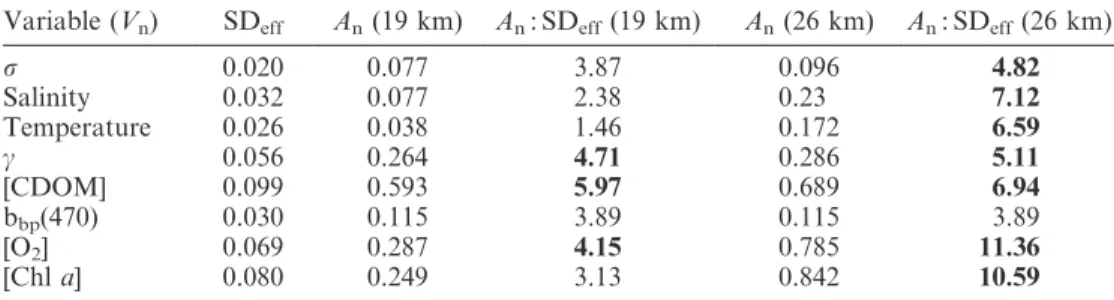
Table 1. Significance ratios (An: SDeff) of anomalies over horizontal section at 120 m. Anis
the amplitude of the normalized variable Vnmeasured from the baseline of the anomaly to its
peak or trough. The effective standard deviation SDeff of Vn is calculated as the standard
deviation of the first difference of Vn. Significant anomalies are in bold and indicated by black
arrows in Fig. 7.
Variable (Vn) SDeff An(19 km) An: SDeff(19 km) An(26 km) An: SDeff(26 km)
s 0.020 0.077 3.87 0.096 4.82 Salinity 0.032 0.077 2.38 0.23 7.12 Temperature 0.026 0.038 1.46 0.172 6.59 c 0.056 0.264 4.71 0.286 5.11 [CDOM] 0.099 0.593 5.97 0.689 6.94 bbp(470) 0.030 0.115 3.89 0.115 3.89 [O2] 0.069 0.287 4.15 0.785 11.36 [Chl a] 0.080 0.249 3.13 0.842 10.59
Table 2. Significance ratios (An: SDeff) of anomalies over horizontal section at 50 m. Anis
the amplitude of the normalized variable Vnmeasured from the baseline of the anomaly to its
peak or trough. The effective standard deviation SDeff of Vn is calculated as the standard
deviation of the first difference of Vn. Significant anomalies are in bold and indicated by black
arrows in Fig. 8.
Variable (Vn) SDeff An(23 km) An: SDeff(23 km) An(32 km) An: SDeff(32 km)
s 0.027 0.119 4.36 0.119 4.36 Salinity 0.037 0.02 0.54 0.378 10.13 Temperature 0.033 0.159 4.85 0.06 1.83 c 0.043 0.253 5.88 0.317 7.37 [CDOM] 0.111 0.398 3.59 0.736 6.63 bbp(470) 0.042 0.299 7.17 0.08 1.92 [O2] 0.081 0.139 1.71 0.836 10.31 [Chl a] 0.079 0.348 4.43 0.796 10.13
possibly associated with some diffusion. Chl a cannot remain in an aphotic environment more than a few days because photosynthesis is not possible there, whereas significant vertical displacement of algae by sedimentation would change the [Chl a] : [O2] ratio. Therefore, high spatial
resolution profiles of non-conservative biogeochemical variables bring information on short-term physical pro-cesses and vertical advection. Such a conclusion could not be obtained if pseudo-conservative variables such as T and S are considered because they do not retain the properties of the initial (source) water mass. However, it cannot be argued that vertical advection occurred either in the plane of the section or during the time period this transect was made; we can only be certain that some days earlier this water mass was near the surface in a productive zone.
The same argument can be used regarding the signature of high CDOM concentration in the surface layers. A nutrient profile taken on 22 Jan 2007 at the DYFAMED/ Boussole station (data not shown) revealed surface values of 1.23 mmol L21, an indication that the central zone was
not nutrient limited. Unfortunately, nutrient measurements were not among those made by the glider and could not be used to reinforce the small-scale interpretation of CDOM anomalies. However, similar zones of high nutrient concentrations in a generally depleted surface layer have already been observed near the Ligurian front in early spring (Sournia et al. 1990). The question now arises as to the kind of physical processes that could explain such localized vertical advection near a frontal zone.
Vertical velocities in the vicinity of geostrophic fronts have already been obtained (Pollard and Regier 1992; Allen et al. 2001) using the omega equation under quasi-geostrophic (QG) approximations and source terms result-ing from geostrophic deformation fields. The omega equation (Hoskins 1982) is derived from the moment equations by considering the time evolution of the imbalance between the two terms of the thermal–wind equations. It is an elliptic equation of the vertical velocity w with the right-hand side terms implying a divergence of source terms Qi. These Qi terms involve along-front, vertical, and cross-front derivatives, thus requiring a three-dimensional data set in a frontal zone in order for the omega equation to be applied.
With only two-dimensional cross-front glider data, such calculations could not be applied. Presently, only the QG omega equation has been applied to oceanic data obtained by Seasoar mapping, occasionally including [Chl a] data (Allen et al. 2005). However, the so-obtained QG w field neglects the ageostrophic advection in Qi terms and could be biased. Generalized omega equations (Viudez et al. 1996) taking into account ageostrophic advection of the main flow can cause important changes due to that advection and will then introduce additional Qi terms that modify secondary circulation. Recently, Giordani et al. (2006) used modeling and generalized omega equations to demonstrated the potential importance of turbulent fluxes as sources of vertical secondary circulation. Before this, Thomas and Lee (2005) showed that surface turbulent fluxes near frontal zones can destroy potential vorticity by gravitational instability in the vicinity of surface fronts when winds, even moderate, blow along the main horizontal current flow. Some geostrophic adjustment then occurs, resulting in multiple vertical circulation cells. Another study (Nagai et al. 2006) showed strong vertical convergences near a front and upwelling in the axis of the jet and, in some cases, in the central zone when (1) winds were blowing along the flow and (2) turbulent fluxes of moments and tracers were parame-terized by variable turbulent viscosity and diffusivity coefficients.
In the case of this transect, as winds blowing from the northeast (in a southwesterly direction along the current flow) are frequently encountered in the Ligurian Sea area, a similar process may be occurring. Based on results such as those of Thomas and Lee (2005) and Nagai et al. (2006), as well as our own analysis, we conclude that our interpre-tation of biogeochemical variables as tracers for frontal vertical circulation induced by along-front winds is coherent in the case outlined in this article. A second compelling indicator is that of the upwelled waters also observed in the frontal zone. Such upwelling occurring along the frontal interface has never been obtained using the classical hypothesis of the quasi-geostrophic omega equation, but could exist using the Thomas and Lee (2005) scenario. If the scenario is correct, anomalies found in the January section when winds were blowing down-flow would not be observed for each monthly section but rather would depend on the wind direction and amplitude.
The nature of particulate material along the transect—In terms of particle load bbp(470), and size (c), there is a clear
partitioning between marginal waters (high backscattering and low c) and central ones (low backscattering and high c) (Fig. 4h,i). Furthermore, whereas [Chl a] and bbp(470) are
related in the central waters (r2 5 0.74, n 5 26,530), no
clear pattern emerges for the marginal ones (Fig. 10b). The same observation applies when comparing c to [Chl a] (Fig. 10a). Such results suggest that distinct typologies in the composition of the particle assemblage occur on each side of the frontal system. The convergence tongues 1 and 2 (Fig. 10a,b) further support this fact, as each tongue lies within a distinct range of bbp(470), c, and [Chl a] values.
In the central zone, the correlation between bbp(470) and
[Chl a] suggests that most of the particles are of a biogenic
Fig. 9. Ratio of [Chl a] : [O2] highlighting the surface-water
sources of each tongue. The primary downwelled tongue (tongue 1) originates in the central WIW waters near the surface (higher values of [Chl a] : [O2]); the secondary smaller tongue (tongue 2)
originates in the MAW of the frontal zone (mid-range values of [Chl a] : [O2]). (Ocean Data View [ODV] Software, version 3.2.2,
nature. This might be due either to a quasi-exclusive dominance of phytoplankton or to a constant proportion of phytoplankton to bbp(470). Furthermore, the higher the
[Chl a], the lower the c, thus the greater the contribution of larger size particles to the particle assemblage. Whether this reflects actual change in the community composition with increasing Chl a (e.g., from a flagellate-dominated toward a diatom-dominated community, a feature already reported for jet-front systems in Claustre et al. 1994b) or corre-sponds to the signature of a richer phytoplankton assemblage (a consequence of more favorable growth conditions) is not possible to ascertain with the present data set. This observation nevertheless points to interesting small-scale nuances in the composition of particles (phyto-plankton pool) in this zone, deserving additional dedicated investigations.
The contribution of phytoplankton to the particle load in the marginal zone is much lower than in the central one. Furthermore, the strong decorrelation between bbp(470) and
Chl a (Fig. 10b), especially over the vertical, suggests that
this contribution is highly variable. The corollary is also that there exists a greater and more variable contribution of non-phytoplankton particles in the marginal zone. These particles are larger (lower c) than in the central area. They can be either biogenic (small detritus, small heterotrophs) or mineral, the latter being the possible result of river run-off or a consequence of a previous intense rain event. Whatever the nature of this non-chlorophyllous material, the present results suggest a clear distinct origin of the particulate material in the central zone from that in the marginal zone. This conclusion cannot be reached for the dissolved material (CDOM), which does not present any clear large-scale trend along the transect. It might be that besides photodestructive processes (and poor CDOM concentrations relative to sensor sensitivity), the characteristic time scales of CDOM dynamics are much larger than the ones involving particle (Chl a and bbp) dynamics.
Finally, at km 25 between the marginal and central waters, a 3-km-wide particle patch (local maximum in bbp[470])
associated with a significant chlorophyll content (0.4 mg m23) and the lowest overall c (highest contribution
of large particles) is recorded on the cyclonic side of the current. This patch is associated with the surfacing of the 28.5 kg m23isopycnal (Fig. 4h,i) and correlates to the core of
the current (Fig. 4a; km 23, 0–50-m depth) where maximum velocities (60 cm s21) are observed. This observation might
be the signature of a local development of large phytoplank-ton or may be a particle concentration or aggregation phenomenon as a result of convergence processes.
Duration and recurrence of structures—Structures such as those described in the sections above were also observed in glider data retrieved during March and May of 2007. The February deployment was made 24 km west of our usual deployment point, and data from this transect showed no convergence tongues.
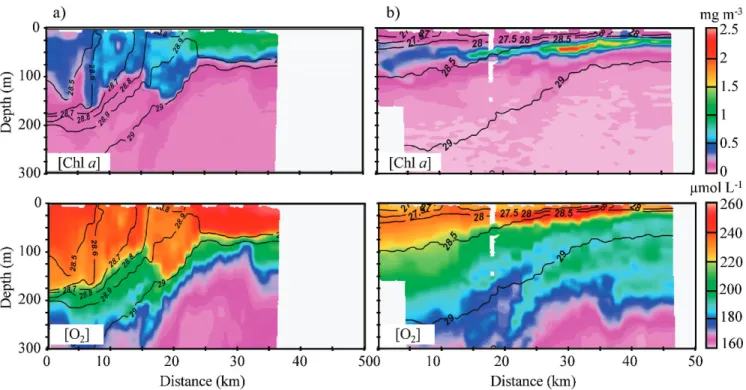
In the March transect (Fig. 11a), an 8-km-wide iso-pycnal [Chl a] tongue (0.55 mg m23) was seen to a depth of
150 m with an associated [O2] tongue having 200 mmol L21
values down to 200 m and 180 mmol L21 values down to
300 m. Northwesterly winds averaged 2 m s21 the week
before deployment, but 9 days earlier winds gusted southwestward for 2 days, attaining speeds of 10 m s21.
During the springtime bloom and stratification (Fig. 11b, May deployment), the deep chlorophyll maxi-mum (DCM) was observed at 50-m depth, just below the 28.5 kg m23 isoline, whereas [Chl a] convergence tongues
were not observed at all. Oxygen concentration still showed obvious traces of a tongue (180 mmol L21) down to 300 m
(Fig. 11b). The distribution of low values throughout the water column is uniform, leaving elevated values primarily near the surface, correlating to the DCM. During this deployment, westerly winds averaged 3 m s21but attained
8 m s21southwestward 12 days beforehand.
It is likely that the relative intensity of tongues in terms of [O2] and [Chl a] at these varying periods are dependent
on the wind history before the glider transects. Strong southwesterly winds occurred only 2 days before the January transect and were maintained throughout the glider mission, probably explaining the strong co-occurring
Fig. 10. (a) Scatterplot of [Chl a] vs. c against potential density s. (b) Scatterplot of [Chl a] vs. bbp(470) against potential
density s. Both figures show a correlation in surface central waters (s 5 28.9–29.0 kg m23) but not in marginal ones (s 5 28.4–
28.9 kg m23); The different regions occupied by tongues 1 (blue)
and 2 (black) superimposed on these figures indicate differences in their respective particulate compositions. (Ocean Data View [ODV] Software, version 3.2.2, R. Schlitzer; http://odv.awi.de/).
signatures of both [Chl a] and [O2]. The absence of
southwesterly winds preceding the February deployment may well explain why such convergence tongues were not observed in this data set (data not shown).
It is very likely that stratification is a factor in reducing or limiting secondary circulation from occurring. On the other hand, the observation of these tongues may also depend on the meandering of the current and the position at which it is intersected by the glider transect. The question then arises as to whether such winter observations of biogeochemical anomalies are representative and recurrent. One would expect them to be, as southwesterly winds (along-front) in the central part of the Ligurian Sea are as frequent as northeasterly winds. Clearly, a model for investigating such alternating modal directions is needed to determine the effect on displacement of fronts and instabilities near the limit between the frontal and central zones. In order to track the evolution of these vertical structures, determine the potential duration and recurrence, and better address the issue of data synopticity (for finescale and evolving structures), a more adapted sampling strategy involving multiple gliders continuously surveying the frontal zone in a large enough area to include meanders would also be necessary.
Some of the biogeochemical variables measured in this study (e.g., CDOM, Chl a) are non-conservative tracers. Their production and removal rates are dependent on photochemical processes like photosynthesis or CDOM photodestruction. These processes have their own charac-teristic time scales, and their magnitude depends on the available irradiance at the actual depth, as well as the irradiance history of the tracer in the water column.
Therefore, the observed fields of such tracers, especially in the restricted zones of upward and downward motion, represent the combined effect of vertical displace-ment rates together with rates of the photo-processes. With the presently available physical instrumentation, the estimation of vertical displacement in such systems is tentative at most. In the past, there have been some attempts at using the knowledge of the time scale of photosensitive processes to provide (rough) estimates of the physical activity responsible for modifying the vertical distribution of the tracer. This has been performed, for example, by using photosensitive tracers like hydrogen peroxide or photoprotective carotenoids (Claustre et al. 1994a; Eisner et al. 2003).
Apparent optical properties (R and Kd) derived from
Tournesol’s radiometric measurements can be further inverted into inherent optical properties (absorption and backscattering coefficient) using appropriate models (Loi-sel and Stramski 2000; Morel et al. 2002; Brown et al. 2004). As the backscattering coefficient is also measured independently, our bio-optical glider represents a powerful and unique platform in view of validating such inversion models or developing more adapted ones. Furthermore, the estimation of the absorption coefficient at four wavelengths in the blue spectral domain may allow partitioning between absorption by CDOM and phytoplankton (Niewiadomska et al. unpubl.). These estimations will complement those relying on CDOM and Chl a fluorescence (access to fluorescence quantum yield, ratio of fluorescence to absorption, for both classes of compounds). A detailed description of this methodology is not within the scope of this article and will be published later.
Fig. 11. Glider transects for 12–14 Mar 2007 and 15–17 May 2007. (a) Glider Chl a concentration and oxygen concentration for March deployment; (b) glider Chl a concentration and oxygen concentration for May deployment. (Ocean Data View [ODV] Software, version 3.2.2, R. Schlitzer; http://odv.awi.de/).
Such new observations have to serve in return as better constraints for the estimation of physical motions. We thus believe that it is timely, in parallel with these new autonomous observations, to reinforce and refine ap-proaches (in situ and laboratory experiments supported by models) aimed at better characterizing the critical time scales of these photosensitive processes.
References
ALLEN, J. T., D. A. SMEED, J. TINTORE, AND S. RUIZ. 2001. Mesoscale subduction at the Almeria-Oran front Part I: Ageostrophic flow. J. Mar. Syst. 30: 263–285.
———,AND oTHERS. 2005. Diatom carbon export enhanced by silicate upwelling in the northeast Atlantic. Nature 437: 728–732.
BOUCHER, J., F. IBANEZ,ANDL. PRIEUR. 1987. Daily and seasonal variations in the spatial distribution of zooplankton popula-tions in relation to the physical structure in the Ligurian sea front. J. Mar. Syst. 45: 133–173.
BROECKER, W. S. 1974. ‘‘NO’’ A conservative water-mass tracer. Earth Planet Sci. Lett. 23: 100–107.
———, T. TAKAHASHI,ANDT. TAKAHASHI. 1985. Sources and flow patterns of deep-ocean waters as deduced from potential temperature, salinity and initial phosphate concentration. J. Geophys. Res. 90: 6925–6939.
BROWN, C. A., Y. HUOT, M. J. PURCELL, J. J. CULLEN,ANDM. R. LEWIS. 2004. Mapping coastal optical and biogeochemical variability using an autonomous underwater vehicle and a new bio-optical inversion algorithm. Limnol. Oceanogr. Methods 2: 262–281.
CLAUSTRE, H., F. FELL, K. OUBELKHEIR, AND L. PRIEUR. 2000. Continuous monitoring of surface optical properties across a geostrophic front: Biogeochemical inferences. Limnol. Ocea-nogr. 45: 309–321.
———, P. KERHERVE´, J. C. MARTY, AND L. PRIEUR. 1994a. Phytoplankton photoadaptation related to some frontal physical processes. J. Mar. Syst. 5: 251–265.
———, ———, ———, ———, C. VIDEAU, AND J. H. HECQ. 1994b. Phytoplankton dynamics associated with a geostrophic front —Ecological and biogeochemical implications. J. Mar. Res. 52: 711–742.
EISNER, L. B., M. S. TWARDOWSKI, T. J. COWLES, AND M. J. PERRY. 2003. Resolving phytoplankton photoprotective: Photosynthetic carotenoid ratios on fine scales using in situ spectral absorption measurements. Limnol. Oceanogr. 48: 632–646.
ESAIAS, W. E., AND oTHERS. 1998. An overview of MODIS capabilities for ocean science observations. IEEE Trans. Geosci. Rem. Sens. 36: 1250–1265.
FASHAM, M. J. R., T. PLATT, B. IRWIN, AND K. JONES. 1985. Factors affecting the spatial pattern of the deep chlorophyll maximum in the region of the Azores front. Progr. Oceanogr. 14: 129–165.
FEDOROV, K. N. 1986. The physical nature and structure of oceanic fronts. Translated from Russian. Springer-Verlag. FIELDING, S., N. CRISP, J. T. ALLEN, M. C. HATMAN, B. RABE,AND
H. S. J. ROE. 2001. Mesoscale subduction at the Almeria-Oran front part 2: Biophysical interactions. J. Mar. Syst. 30: 287–304.
FOFONOFF, N. P.,ANDR. C. MILLARD, JR. 1983. Algorithms for computation of fundamental properties of seawater. UN-ESCO Technical Papers in Marine Science 44. Available online at <http://unesdoc.unesco.org/images/0005/000598/ 059832EB.pdf>.
FRANKS, P. J. S. 1992. Phytoplankton blooms at fronts: Patterns, scales and physical forcing mechanisms. Rev. Aquat. Sci. 6: 121–137.
GIORDANI, H., L. PRIEUR, AND G. CANIAUX. 2006. Advanced insight into sources of vertical velocity in the ocean. Ocean Dynam. 56: 513–524.
HOSKINS, B. J. 1982. The mathematical theory of frontogenesis. Annu. Rev. Fluid Mech. 14: 131–151.
JOHNSON, K. S., S. W. WILLASON, D. A. WIESENBURG, S. E. LOHRENZ,ANDR. A. ARNONE. 1989. Hydrogen peroxide in the western Mediterranean Sea: A tracer for vertical advection. Deep-Sea Res. 36: 241–254.
LE´ VY, M. 2003. Mesoscale variability of phytoplankton and of new production: Impact of the large-scale nutrient distribu-tion. J. Geophys. Res.-Oceans 108: C113358, doi: 3310.1029/ 2002JC001577.
———, P. KLEIN, AND A. M. TREGUIER. 2001. Impact of sub-mesoscale physics on production and subduction of phyto-plankton in an oligotrophic regime. J. Mar. Res. 59: 535–565. LOISEL, H., J.-M. NICOLAS, A. SCIANDRA, D. STRAMSKI, AND A. POTEAU. 2006. Spectral dependency of optical backscattering by marine particles from satellite remote sensing of the global ocean. J. Geophys. Res. 111: C09024, doi: 09010.01029/ 02005JC003367.
———,ANDD. STRAMSKI. 2000. Estimation of the inherent optical properties of natural waters from the irradiance attenuation coefficient and reflectance in the presence of Raman scattering. Appl. Optic. 39: 3001–3011.
MILLOT, C. 1999. Circulation in the Western Mediterranean Sea. J. Mar. Syst. 20: 423–442.
MOREL, A., D. ANTOINE, AND B. GENTILI. 2002. Bidirectional reflectance of oceanic waters: Accounting for Raman emission and varying particle scattering phase function. Appl. Optic. 41: 6289–6306.
———,ANDJ. BERTHON. 1989. Surface pigments, algal biomass profiles, and potential production of the euphotic layer: Relationships reinvestigated in view of remote-sensing appli-cations. Limnol. Oceanogr. 34: 1542–1562.
———, AND S. MARITONERA. 2001. Bio-optical properties of oceanic waters: A reappraisal. J. Geophys. Res. 106: 7163–7180.
MORISON, J., R. ANDERSEN, N. LARSON, E. DASARO,ANDT. BOYD. 1994. The correction for thermal-lag effects in Sea-Bird CTD data. J. Atmos. Ocean. Tech. 11: 1151–1164.
NAGAI, T., A. TANDON, AND D. L. RUDNICK. 2006. Two-dimensional ageostrophic secondary circulation at ocean fronts due to vertical mixing and large-scale deforma-tion. J. Geophys. Res. 111: C09038, doi: 09010.01029/ 02005JC002964.
NURSER, A. J. G., ANDJ. W. ZHANG. 2000. Eddy-induced mixed layer shallowing and mixed layer/thermocline exchange. J. Geophys. Res. 1005: 21851–21868.
PINOT, J. M., J. TINTORE, J. L. LOPEZJURADO, M. L. F. DEPUELLES, AND J. JANSA. 1995. Three-dimensional circulation of a mesoscale eddy/front system and its biological implications. Oceanol. Acta 18: 389–400.
POLLARD, R.,ANDJ. READ. 1989. A method for calibrating ship-mounted acoustic doppler profilers and the limitations of gyro compasses. J. Atmos. Ocean. Tech. 6: 859–865.
POLLARD, R. T.,ANDL. A. REGIER. 1992. Vorticity and vertical circulation at an ocean front. J. Phys. Oceanogr. 22: 609– 625.
PRIEUR, L. 1979. Structures hydrologiques, chimiques et biologi-ques dans le bassin Liguro-Provenc¸al. Rapp. Comm. Int. Mer Me´dit 25/26: 75–76.