S. Borguet
e-mail: [email protected]P. Dewallef
e-mail: [email protected]O. Léonard
e-mail: [email protected] Turbomachinery Group, University of Liège, Chemin des Chevreuils 1, 4000 Liège, BelgiumA Way to Deal With Model-Plant
Mismatch for a Reliable
Diagnosis in Transient Operation
Least-squares health parameter identification techniques, such as the Kalman filter, have been extensively used to solve diagnosis problems. Indeed, such methods give a good estimate provided that the discrepancies between the model prediction and the measure-ments are zero-mean, white, Gaussian random variables. In a turbine engine diagnosis, however, this assumption does not always hold due to the presence of biases in the model. This is especially true for a transient operation. As a result, the estimated parameters tend to diverge from their actual values, which strongly degrades the diagnosis. The purpose of this contribution is to present a Kalman filter diagnosis tool where the model biases are treated as an additional random measurement error. The new methodology is tested on simulated transient data representative of a current turbofan engine configura-tion. While relatively simple to implement, the newly developed diagnosis tool exhibits a much better accuracy than the original Kalman filter in the presence of model biases. 关DOI: 10.1115/1.2833491兴Keywords: engine health monitoring, Kalman filter, model-plant mismatch
Introduction
The diagnosis tool considered herein is basically a gas path analysis method whose purpose is to assess the deviations of some health parameters on the basis of measurements collected within the gas path of the engine关1兴. The health parameters are coeffi-cients affecting the efficiency and the flow capacity of the com-ponents共fan, low pressure compressor 共lpc兲, high pressure com-pressor 共hpc兲, high pressure turbine 共hpt兲, low pressure turbine 共lpt兲, and nozzle兲, while the measurements are intercomponent temperatures, pressures, as well as rotational speeds. The health assessment leads to a diagnosis of the engine condition, which allows suitable maintenance actions to be undertaken.
The health parameter estimation is achieved by a Kalman filter, which is a minimum mean square error 共variance兲 estimator within a recursive framework关2兴. This means that the estimated health parameters minimize the distance 共in the least-squares sense兲 between a model prediction and the observed measure-ments. Moreover, the recursive structure of the Kalman filter up-dates the values of the identified health parameters as new data are available, which is a useful property in real-world applications such as on-board performance monitoring关3兴.
Since the first research efforts of Urban 关4兴, most of the gas path analysis methods were restricted to measurements observed under steady-state operation of the engine, mainly for computa-tional load reasons. For a few years, the ability to extract the engine condition from transient data has been investigated using various techniques such as least-squares estimation关5,6兴, artificial neural networks关7兴 for a batch treatment of the data, and Kalman filters关8–11兴 in a recursive framework.
More specifically, it has been shown in Ref.关10兴 that the use of measurements representative of transient behavior significantly improves both the diagnosis accuracy and the isolation capability under negative redundancy共i.e., more health parameters than sen-sors兲, provided that a faithful dynamic model is available. Indeed, a transient operation allows a much greater number of operating points to be considered, thereby increasing the analytical redun-dancy.
Although the existence of a perfectly faithful model is generally assumed, this hypothesis is rarely met in practice. In fact, complex phenomena, such as heat transfer, volume dynamics, clearances, and secondary airflow and power off-takes, are poorly modeled or unmodeled in current state-of-the-art aerothermodynamic engine models关12,13兴. Consequently, the performance predictions gener-ated by the dynamic model are biased with respect to measure-ments taken on the engine. As reported in Ref.关11兴, those biases strongly reduce the efficiency of the diagnosis tool.
The present contribution proposes a solution to the model bi-ases by considering them as an additional measurement error. In-deed, from the point of view of an external observer, it is not possible to distinguish a model bias from a sensor error. However, unlike sensor errors, which are basically unpredictable before-hand, the model biases of interest have a more predictable nature that can be studied by comparing the model outputs and the mea-surements observed on a healthy engine during a learning phase previous to the health parameter assessment.
Description of the Method
The scope of this section is to provide a short description of our diagnosis tool and to present the methodology we have developed to cope with model-plant mismatch and its integration within the diagnosis algorithm.
Diagnosis Tool. Our diagnosis tool belongs to the family of model-based approaches, meaning that a simulation model of the turbine engine must be available. In the framework of gas path analysis, these are basically nonlinear aerothermodynamic models based on mass, energy, and momentum conservation laws applied to the engine.1
As mentioned in the Introduction, the framework in which this contribution takes place is the development of a diagnosis tool processing transient data and reliance on the Kalman filter estima-tion algorithm. Since the system model is nonlinear, the unscented Kalman filter关14兴 is used instead of the generic linear Kalman filter. A few adjustments and assumptions govern the applicability
Manuscript received June 20, 2006; final manuscript received October 29, 2007;
published online March 26, 2008. Review conducted by Jeffrey W. Bird. 1Linearized models are often used to lower the computational burden.
of the unscented Kalman filter. The first one consists in formulat-ing the simulation model of the engine in terms of a state-space model, namely,
xk=F共uk,vk,wk,xk−1兲 +k 共1兲 yk=G共uk,vk,wk,xk兲 +⑀k 共2兲
where k is a discrete time index, ukare the command parameters 共e.g., fuel flow兲, vkare measurable exogenous inputs共e.g., Mach
number and altitude兲, wk are the aforementioned health param-eters, and xk are the state variables. The state variables are
in-tended to handle the transient effects taking place in the gas path of the engine. Generally speaking, these transient effects belong to three categories, namely, the heat transfers between the gas path and the components of the engine, the shaft inertia, and the fluid transport delays.
Equation共2兲 is called the measurement equation and joins the deterministic simulation modelG共·兲 and a random variable⑀k
in-tended to represent the stochastic influence of the measurement uncertainties. Similarly, Eq. 共1兲 is named the state prediction equation and links the deterministic integration routineF共·兲 of the simulation model and a random variablek, which represents an error term. In addition to these two equations, a third one, named the health parameter transition equation, is often included which states that the health parameters may vary in time by following a first-order Markov process共see Ref. 关3兴 for further details兲.
The second assumption is that both k and⑀k are zero-mean,
white, and Gaussian random variables2which is denoted by ⑀k=N共0,Ry兲 and k=N共0,Rx兲 共3兲
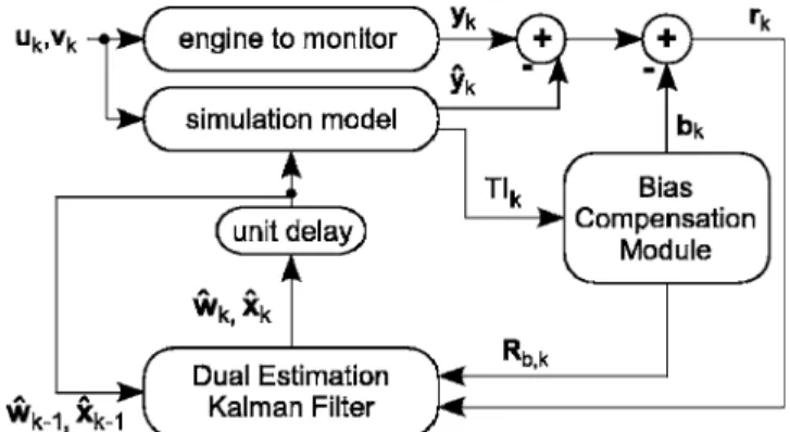
Since the state variables are unknown共not all of them are mea-surable兲, they must be estimated together with the health param-eters from the same sequence of measurements yk. This problem, known as the dual estimation problem, is solved herein by a so-called dual estimation Kalman filter共DEKF兲. This dual Kalman filter relies on two unscented Kalman filters running concurrently, one for the health parameters and the other for the state variables. The interested reader may consult Ref.关15兴 for a detailed descrip-tion of the algorithm. Basically, once the former filter has updated the health parameters, the current value is used by the latter to update the corresponding state variables.
Provided that a prior value for the health parameters and the state variables is available, the basic step consists of observing the discrepancies between the model outputs, denoted by yˆk, and the
observed measurements yk. These discrepancies, also called re-siduals and denoted by rk, are processed by the DEKF, which
recursively updates the health parameters and the state variables so that the average value of rkis driven to zero. In other words,
the identified health parameters provide a means of observing the actual health condition of the engine. Figure 1 summarizes this recursive, closed-loop process. The engine performance model, actually embedded in the DEKF, has been represented outside of it in order to underline its important role in the estimation process. Dealing With Model Biases. The physical meaning of the identified health parameters is only valid provided that the model is faithful. Otherwise, as reported by Volponi in Ref. 关11兴, the health parameters become “tuners,” which are adjusted by the identification process to fit the behavior of the real engine, losing sense for diagnosis reports. Indeed, as formulated in the preceding section, the Kalman filter assumes that the discrepancies between the model and the measurements are zero on average.
Unfortunately, model biases do not have a pure stochastic na-ture, but should rather be seen as systematic errors whose mean values are different from zero. The assumption on the noise char-acteristics is therefore violated, which perturbs the health
param-eter identification. In practice, it has been observed that model biases as small as the measurement noise standard deviation can dangerously reduce the reliability of the diagnosis. Therefore, the biases have to be modeled in some way so that the residuals will reflect only the degradation of the engine. In reality, the model-plant mismatch depicts the approximations made in both the state transition equation共Eq. 共1兲兲 and the measurement equation 共Eq. 共2兲兲. A possible mathematical translation of this fact is to consider that neither⑀knorkare zero-mean, Gaussian random variables. In this contribution, it is proposed to gather all the effects caused by modeling errors in the single measurement equation 共Eq. 共2兲兲. The measurement noise ⑀k is now seen as a hybrid
bias-noise term gathering the measurement noise and the model-plant mismatch. Mathematically speaking, ⑀k is considered as a
Gaussian random variable of variable properties共i.e., mean and covariance兲. Two reasons favored this choice: First, the Kalman filter deals with this type of random variables. Second, a Gaussian random variable is totally defined by its mean and its covariance, which is simple to handle in practice,
⑀k=N共bk,Rb,k兲 共4兲
Provided that bkand Rb,kare known, the mechanism of the
un-scented Kalman filter can be applied by making the following substitutions:
rk= yk− yˆk→ rk= yk− yˆk− bk 共5兲
Ry→ Rb,k 共6兲
Determination of bkand Rb,k. As already mentioned above, the model biases are not, strictly speaking, random variables. Con-sequently, they can be studied beforehand, for example, during the acceptance tests that every engine undergoes before it is brought into service. The purpose of this offline learning is to build a model that predicts bk and Rb,k as precisely as possible. This
approach is very close to the eStorm philosophy 关11兴, with the difference that in our study both the mean bias and its uncertainty are modeled.
During this learning phase, model outputs are compared to the observed measurements without estimating the health parameters, which are assumed to be at their healthy nominal values. As the engine transient model is not perfect, the observed residuals rk
correspond to the model biases. The next step of the learning phase consists of characterizing the mean bk and the covariance matrix Rb,kof the observed biases.
2
In addition,kand⑀kare assumed uncorrelated.
Fig. 1 Health parameter and state variable update mechanism using a DEKF
Modeling the mean bias bkis typically a function approxima-tion problem. In the following, some general consideraapproxima-tions about this problem are recalled. Numerous textbooks address this prob-lem in a more exhaustive way共see, for instance, Ref. 关16兴兲.
The cloud of data of the learning set has to be fitted with a functionH, which may depend on the controls, the ambient vari-ables, the state varivari-ables, and, possibly, past values of them and which also contains fitting parameters p, as stated in
bk=H共uk,vk,xk, . . . ,p兲 共7兲
The first step is to decide on which input variables the functionH depends, with the aim of reducing the dimensionality of the input space by performing a so-called feature extraction. A feature can be seen as an intelligent transformation of the original input vari-ables. Then, the structure共e.g., polynomial fit or neural networks兲 and the complexity 共e.g., order of the polynomial or number of hidden nodes兲 have to be selected. As a result, the number of fitting parameters p is obtained. For example, in the case of a scalar, second-order polynomial fit, the fitting parameters p are the three coefficients of the parabola.
The choice of the flexibility of the fitting function must be done in a very careful way. Indeed, the goal is to obtain the best repre-sentation of the underlying properties of the data in the learning set and hence to obtain the best generalization performance. In other words, over-fitting of the data must be avoided. So, the number of samples in the learning set should be large enough with respect to the flexibility of the approximation function. On the other hand, a general result of learning theory states that for a given number of fitting parameters, the larger the database, the more meaningful the values of these parameters from a statistical point of view共see Ref. 关16兴兲.
The fitting parameters p are generally computed through the minimization of an error function共e.g., sum of squares error兲. The determination of the covariance matrix Rb,k is to be explained
later.
Considering the present application, a rather basic, but physi-cally meaningful, model is chosen. First, fixed ambient conditions 共e.g., sea-level static兲 are selected when collecting the learning set. Then, three assumptions are made in order to simplify the determination of bkand Rb,k.
1. The engine steady-state model is highly accurate. To this end, model-matching techniques such as those described in Refs.关17兴 or 关18兴 can be applied.
2. The engine undergoes moderate transient maneuvers. This constraint can be expressed in terms of an upper limit on the engine acceleration. This bound is application dependent and was set here for the sake of simplicity to a value of ⫾200 rpm/s on the fan rotor acceletation.3
3. During the learning phase, the engine is in healthy nominal condition, hence the values of the health parameters are known and set to their nominal values.
The problem of modeling the mean bkis first investigated. We
can reasonably suppose that the more rapid and complex the tran-sient is, the greater the model-plant mismatch is. Therefore, it is desirable to link the mean bias bkto a scalar quantity, which is
representative of the “intensity” of the transient and which is easy to compute. To this end, the following transient index 共TI兲 is defined: TIk= 1 nx
兺
i=1 nx xˆ˙k共i兲 xref共i兲 共8兲where nx is the number of state variables of the on-board model, xˆ˙k共i兲 is the derivative of state variable i at time index k, and xref共i兲
is the reference value of state variable i共e.g., at take-off rating兲. The unit of TI is s−1. The normalization by a reference state value is required given the different orders of magnitude of the state variables. The TI is zero in a steady-state operation, positive when the engine is accelerating, and negative otherwise.
The TI is computed based on state derivatives provided by the engine model rather than on actual measurements. Two reasons dictate this choice: First, the engine model produces noise-free signals and outputs directly the state derivatives; second, not all state variables are normally measurable on the real engine共e.g., the metal temperatures involved in the heat transfers兲 but are available in the engine model.
So, modeling the mean value of the bias amounts to determin-ing the mappdetermin-ing bk= f共TIk兲 from the database of biases. This
prob-lem is solved through a least-squares polynomial fit. The selection of the polynomial order and a possible partitioning of the TI axis is a question of engineering judgment. Additional indications are provided in the application detailed later in the paper.
The model of the mean value of the bias available, the covari-ance matrix of the bias, Rb,k, can now be computed. The
proce-dure is given in Algorithm 1. Depending on the partitioning adopted for the mean bias, one covariance matrix is computed per TI segment. As a first step, the gap between each data point and the mean bias is computed for all data points belonging to a par-ticular segment 共lines 2–5, note that each vector ei is a ny⫻1
vector兲. Finally, each element of the symmetric covariance matrix is obtained using the well-known definition of the covariance of random variables共line 6兲.
Algorithm 1. Covariance matrix computation.
1. Set N = 0
2. for all k such that TImin⬍TI
k艋TImaxdo 3. N = N + 1 4. eN= rˆk− b共TIk兲 5. end for 6. Rb= 1 N − 1兺i=1 N 兵e iei T其
The covariance matrix takes into account both the measurement noise 共sensor inaccuracies兲 and the possible variability of the mean bias. Also, it should not be surprising that some off-diagonal terms of that matrix are nonzero. This simply indicates that the sensor biases are interdependent as the modeling errors introduce some relationships between the measurements: for instance, the bias on the exhaust gas temperature共EGT兲 sensor measurement is linked to that of the low pressure spool speed since temperature recovery factor for thermocouples will vary with mass flow.
This concludes the offline modeling of the bias model, which can now be integrated within the diagnosis algorithm in order to make it more robust to model-plant mismatches.
Modification of the Diagnosis Algorithm. The block diagram of the modified diagnosis algorithm is shown in Fig. 2. A short
3
Note that another indicator of engine acceleration could be chosen, e.g., core acceleration.
Fig. 2 Integration of the BCM
description of the procedure is given in this section. Similar to the original procedure detailed in Fig. 1, the previous estimates of the state variables xˆk−1and health parameters wˆk−1are used together
with the current inputs ukand vkby the engine performance model to generate an estimation of the measurements. Additionally, the TIkis computed using relation共8兲. From this TI, the mean bias bk
and its covariance matrix Rb,kare obtained according to the bias
model previously set up. The bias bkis taken into account in the residual rk, which is fed into the original DEKF, with the only
difference that the measurement noise covariance matrix Ry is replaced by Rb,k. Loosely speaking, the mean bias bk and its covariance matrix Rb,kare now extra inputs to the original DEKF.
The integration of the bias compensation module 共BCM兲 within the diagnosis algorithm has a very limited impact on the compu-tational load. Indeed, only a polynomial evaluation is used to re-turn bkand Rb,k.
Application of the Method
Engine Configuration. The application used as a test case is a high bypass ratio mixed-flow turbofan. The engine layout is de-scribed in Fig. 3 where the health parameter location and the station numbering are also indicated. One command variable, which is the fuel flow rate fed in the combustor, is considered in the following.
The engine performance model has been developed and vali-dated as part of the OBIDICOTE4project. A detailed description of the model can be found in Ref.关19兴.
As real data were not available, we worked with simulated data only. To introduce modeling errors, we considered two different configurations of the OBIDICOTE model with regard to transient operation. Our hypothesis concerning the perfect fidelity of the steady-state model to the data used is hence implicitly satisfied.
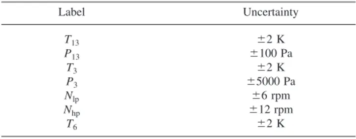
The sensor configuration adopted in the test cases is represtative of typical instrumentation available on modern turbofan en-gines and is detailed in Table 1. The stated uncertainties have been selected according to the OBIDICOTE documentation and ac-count for the magnitude of random errors only.
“Real” Engine and On-Board Model. The OBIDICOTE model plays the role of the “real” engine. The shaft dynamics and the heat transfers in the hpc, burner, and hpt are thus supposed to be perfectly modeled. The seven state variables involved in this first model are listed in Table 2.
Gaussian noise, whose magnitude is specified in Table 1, is added to the clean measurements generated by the real engine model to make them closer to typical test data. The sampling rate
is set to 50 Hz, which is a typical value to capture the transient effects described above.
A second model is embedded in the diagnosis algorithm and plays the role of the imperfect on-board model. It suffers from model-plant mismatch since the heat transfer processes are poorly modeled with respect to the real engine. As shown in Table 3, only three state variables are involved in this second model. They are related to the spool inertia and to a bulk heat transfer in the hpt.
Heat transfer processes are the slowest dynamics in a turbine engine and they quite strongly influence the transient response of the engine共see Ref. 关13兴兲. Considering the present application, the heat transfer is placed on the hpt since it is the hottest part of the engine; therefore, the thermal effects are expected to be more important than in other components. Moreover, the observability of the hpt thermal state is satisfactory with the selected sensor suite共see Ref. 关10兴兲.
Modeling the Bias. The methodology for bias modeling de-scribed in a previous section is applied to the turbofan layout. The task of bias modeling is obviously application dependent. Re-ported here are the main issues of the process for the real engine and on-board model setup.
The first step is to build a database of residuals for the healthy engine, which will serve as a learning set for determining the bias model. Figure 4 depicts the fuel flow trajectory input to the real engine and the on-board model. In this contribution, the engine model is run in open loop; therefore, the set point is specified in terms of fuel flow rather than fan speed or engine pressure ratio. For reference, the lowest fuel flow value 共slightly less than 0.2 kg/s兲 corresponds to the ground idle rating, and the greatest one共slightly higher than 1.2 kg/s兲 gives the take-off power rating. The sequence is 1900 s long so that the database contains 95,000 samples共per sensor兲. Other scenarios could be added to the data-base.
4
A Brite/Euram project for on-board identification, diagnosis, and control of tur-bofan engine.
Fig. 3 Turbofan layout with station numbering and health pa-rameter location
Table 1 Sensor configuration and assumed uncertainty
Label Uncertainty T13 ⫾2 K P13 ⫾100 Pa T3 ⫾2 K P3 ⫾5000 Pa Nlp ⫾6 rpm Nhp ⫾12 rpm T6 ⫾2 K
Table 2 State variables for the real engine
Label Description
Nlp Low pressure spool rotational speed
Nhp High pressure spool rotational speed
Tm3b hpc blade temperature
Tm3c hpc casing temperature
Tm4b Combustion chamber casing temperature
Tm42b hpt blade temperature
Tm42c hpt casing temperature
Table 3 State variables for the on-board model
Label Description
Nlp Low pressure spool rotational speed
Nhp High pressure spool rotational speed
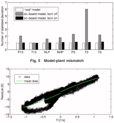
The mismatch between the real engine and the on-board model appears in Fig. 5, where the normalized root mean square error 共NRMSE兲 is plotted for each sensor. The NRMSE for the ith sensor is defined according to
NRMSE共i兲 =
冑
1 n − 1兺
k=1n
共yk共i兲 − yˆk共i兲兲2 Ry共i,i兲
共9兲 As can be seen in Fig. 5, the NRMSE should be equal to 1 if the on-board model were perfect共white bars兲. Indeed, in that case, the only source of variation in the response of the real engine and the on-board model is the sensor noise. For the incomplete on-board model considered in this application 共gray bars兲, it can be seen that the prediction for T13is quite faithful; modeling errors, how-ever, have a significant effect on the other measurements and par-ticularly on T3. Note that the T3prediction error could be reduced by introducing heat transfer on the hpc.
Now, the job consists in defining a model for the residuals from the real and BCM-off data. Plotted in Fig. 6 is the cloud of T3 residuals共black circles兲 with respect to TI for the operation of the engine under the inputs of Fig. 4.
After examining the residual cloud of each measurement, it was decided to split the TI axis into three distinct regions and to apply a quadratic least-squares fit on the data to determine the mean bias
共green lines in Fig. 6兲. The covariance matrices were then com-puted using Algorithm 1. Higher-order polynomials were rejected since the aim is to extract the global trend in the bias.
The resulting bias model is summarized in Table 4. TI쐓 is a threshold value共set to 10−3in this application兲 that makes oper-ating points with small absolute values of TI considered as steady-state ones. For these operating points, the mean bias is set to zero and the covariance matrix Rb,kreduces to the original
measure-ment noise covariance matrix Rygiven the assumption of a per-fect steady-state model. The vectors p1, p2, p3 and p4, p5, p6 are the coefficients of the quadratic least-squares fit for the TI⬎TI쐓 and TI⬍−TI쐓regions, respectively.
The effect of the BCM on the prediction error can be seen in Fig. 5. The black bars represent the NRMSE for each sensor when the BCM is turned on. Obviously, the simple model defined above enhances the accuracy of the prediction provided by the on-board model as all NRMSEs are closer to unity than when the BCM is disabled共gray bars兲.
Test-Case A: Diagnosis at Test Bench. To assess the improve-ments brought by the BCM, the following test case has been de-veloped: It is representative of a maintenance session on a test bench for which sea-level static 共SLS兲, standard day conditions are assumed. The evolution of the fuel flow with respect to time is sketched in Fig. 7. It is an 800 s sequence made of two successive power sweeps between idle and max-continuous regimes, fol-lowed by an acceleration between idle and part-power regimes.5
Engine deterioration is simulated from the component fault case proposed in Ref.关20兴. It consists of a deviation of nearly all health parameters at t = 0 s with the following magnitude: −1.5% on SW12R, −1.2% on SE12, −1.0% on SW2R, −1.0% on SE2, −2.3% on SW26R, −1.4% on SE26, +0.88% on SW41R, −1.6% on SE41, and −1.3% on SE49.
The evolution of the health parameters identified with the origi-nal DEKF共i.e., with the BCM disabled兲 is plotted in Fig. 8. The health parameters exhibit an erratic behavior. Clearly, little valu-able information about the health condition of the engine can be derived from the graphs. The health parameters are used by the DEKF as tuners to drive the residuals to zero共on average兲. The health parameters of the hpc and both turbines seem to be particu-larly sensitive to the model-plant mismatch.
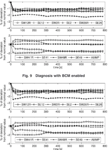
When the BCM is enabled, the identification of the health pa-rameters is depicted in Fig. 9. The improvement with respect to the disabled-BCM case is obvious. The health parameters do not
5
Recall that the engine is open loop, fuel flow piloted.
Fig. 7 Fuel flow profile, test bench conditions Fig. 4 Fuel flow profile for learning set generation
Fig. 5 Model-plant mismatch
Fig. 6 Mean bias extraction for T3
Table 4 Summary of the bias model
Region Mean bias Covariance matrix
TIk⬎TI쐓 bk= p1TIk2+ p2TI+ p3 Rb,kper Algorithm 1
TIk⬍−TI쐓 bk= p4TIk
2
+ p5TI+ p6 Rb,kper Algorithm 1
兩TIk兩⬍TI쐓 bk= 0 Rb,k= Ry
wander according to the transient but converge to their actual value, and the actual condition of the engine can be stated. About 300 s is required to converge to the actual engine health as can be noted on the lower graph reporting the health parameters of the hot section. The small variations in SW26R, SE26, and SW41R are due to the remaining modeling error on T3共see Fig. 5兲.
To underline the originality of our approach that models the mean bias level, and also the uncertainty associated with this bias 共through the covariance matrix Rb,k兲, Fig. 10 depicts the
identifi-cation of the hpt degradation when using a hybrid BCM setting. The mean bias is computed based on the model presented in Table 4, but the covariance matrix of the measurement is set to Rb,k
= Ry, whatever the TI value is. In doing so, no information about the accuracy of the bias bkis transmitted to the DEKF. This
cor-responds to the assumption that bk perfectly matches the model
bias.
These results are much better than those presented in Fig. 8 where the BCM was totally disabled. This hints at the fact that the mean bias has indeed the most disruptive effect on the diagnosis algorithm. Yet, some instabilities are still present in Fig. 10, which disappear when the covariance matrix Rb,kis used共i.e., in Fig. 9兲. This can readily be seen by comparing the smoothness of the curves between Figs. 10 and 9.
From this last result, it can be concluded that even if the mod-eling of the bias is quite simple and not always very accurate, taking the uncertainty in the bias into account can improve the quality of diagnostics. Hence, the role of the covariance matrix Rb,kin the Kalman filter algorithm is to deemphasize the influ-ence of the residuals on the health parameter update when a model bias is likely to be expected or when our knowledge about the bias is not very accurate.
Adapting the Bias Compensation Module to Non-Sea-Level Static Conditions. In the previous subsection, the positive effect of the BCM on the diagnosis algorithm has been demonstrated. The diagnosis was performed in the same atmospheric conditions as for the extraction of the bias model共i.e., SLS conditions兲. Prac-tically, it is indeed difficult to collect biases outside of a pass-off test. Hence, it would be highly valuable to use the predefined BCM for any other operating conditions.
The extension of the BCM to the whole flight envelope of the engine is nearly immediate by having recourse to the concept of corrected parameters, which relies on similarity laws and first-order approximation of the gas turbine aerothermodynamic pro-cesses. The basic idea behind similarity laws is to define dimen-sionless groups of parameters that are associated with the flow field in the engine. Those corrected parameters allow a compari-son, generally on a Mach number basis, of the performance of the engine operating under different atmospheric conditions. As a re-minder, the general expression for the corrected parameter X is given by
Xco= X
a␦b 共10兲
where =T2/Tref, ␦= P2/ Pref, Tref= 288.15 K, and Pref = 101,325 Pa.
Parameter correction is a common practice in the gas turbine community, and the theoretical values of the exponents a and b for the steady-state and transient variables of interest can be found in many references共See, for instance, Refs. 关21,22兴.兲 Yet, addi-tional physical phenomena, such as the modification of the ther-mophysical properties of the working fluid, Reynolds number ef-fects, and geometrical effects共e.g., clearance and blade untwist兲, make the engine behavior deviate from the assumptions of the Mach number similarity. Hence, a fine tuning of the a and b exponents for each parameter involved in the BCM should be carried out as explained in Ref.关23兴 for improved accuracy.
The following operations allow the adaptation of the original BCM to any ambient conditions.
1. Get current state derivatives from the on-board model. 2. Compute corrected state derivatives.
3. Build corrected TI from corrected state derivatives accord-ing to Eq.共8兲.
4. Call the BCM with corrected TI on input; get bkand Rb,kon
output.
5. “Decorrect” bkto current ambient conditions.
As can be noted in item 5, the mean bias bkis decorrected, but not
its associated covariance matrix. Hence, we implicitly assume that the uncertainty in the mean bias is constant for different ambient conditions. It means that the highest contribution to the
measure-Fig. 8 Diagnosis with BCM disabled
Fig. 9 Diagnosis with BCM enabled
ment covariance is the measurement noise 共the magnitude of which is independent of the operating conditions兲 rather than the uncertainty in the mean bias. It is worth mentioning that these adaptations are applied outside of the core of the BCM, which is thereby not affected at all.
Test-Case B: Validation for Non-Sea-Level Static Conditions. To validate the correction procedure applied to the BCM, a second test case has been designed. Cruise flight condi-tions 共altitude=10,800 m, flight Mach number=0.82兲 are as-sumed. The simulated fault is the same engine deterioration as previously described. The open-loop scheduled fuel flow is plotted in Fig. 11 and is similar in shape to the one of test-case A. The reader will certainly notice the simplified nature of this test case, which is intended here for validation purposes only.
Figure 12 sketches the evolution of the identified health param-eters when using the corrected BCM. It can be seen that the en-gine deterioration is accurately assessed共localization and magni-tude兲. As for the identification under SLS conditions, one can notice slight oscillations in SW26R, SE26, and SW41R due to the remaining prediction error in T3.
For the considered application, it can thus be stated that first-order corrections brought by corrected parameters appear to be sufficient to use the original BCM, determined from SLS data, for monitoring the condition of the engine under other ambient con-ditions. It can be explained by the fact that the shortcomings of the model are intrinsic and hence do not depend on the atmo-spheric conditions. The proposed methodology for bias compen-sation is therefore very appealing, given that it is much easier to collect biases on the test bench than in flight.
Discussion
The enhancement of the diagnosis capabilities possible with the BCM in the presence of model-plant mismatch has been discussed in the previous section. However, some more issues have to be discussed to complete the analysis of the results.
The first question is related to the continuity of the bias model with respect to the TI. In this paper, three different TI patterns have been defined, and both the mean bias b and the covariance Rb are discontinuous between adjacent patterns. No instabilities
of the DEKF have been noticed so far. It is supposed that the DEKF is unaware of those discontinuities because it is not sensi-tive to the derivasensi-tive of the bias model. TI segments might be developed to match the specific acceleration and deceleration fea-tures of a particular control system共fuel control and actuators兲.
Another open question is linked to the complexity of the bias model. A very simple piecewise quadratic bias model has been considered in this application, and it has been shown to be suffi-cient for providing a rather accurate diagnosis. However, more complex models, such as neural networks, could be tested. An-other research direction concerning the complexity of the bias model is the definition itself of that model. Throughout the paper, it has been assumed that the bias model only depends on the TI. A formulation with two input arguments such as TI and its time derivative, or TI and a state index, should be investigated. Data mining techniques could be used to this end.
An essential work is to further investigate the applicability of the BCM, defined from SLS mismatch data, throughout the flight envelope. This approach has been proven successful for the par-ticular application considered in the present study, somewhat sim-plified with respect to real-world situations. Indeed, new-generation engines are more complex, from the standpoint of architecture as well as control systems. The structure of the model-plant mismatch might then depend on the ambient and op-erating conditions, too. In that case, collection of mismatch data in an altitude test facility and/or on a flying test bed would become mandatory for a complete determination of the BCM.
Finally, some more studies still need to be undertaken concern-ing robustness issues. Those are twofold: First, the capability of the algorithm to cope with sensor malfunctions is still under de-velopment. Second, the applicability of the methodology pre-sented herein has to be verified for other modeling errors such as sensor/actuator dynamics, fluid dynamics effects, bleed air and power take-offs, and especially biased steady-state engine model-ing.
Conclusion
The ability to perform a reliable diagnosis in transient operation with an imperfect model of a gas turbine has been investigated. A methodology has been developed to compensate for the bias in-duced by model-plant mismatch by treating it as a pseudo-Gaussian variable. The improvements to the quality of the diag-nosis with the new algorithm have been demonstrated on simple, but realistic test cases.
More specifically, it has been pointed out that taking into ac-count both the mean bias and its related uncertainty improves the identification procedure in terms of stability and accuracy even with a rather simple structure of the bias model. The BCM, built from data gathered on a test bench, has also shown interesting generalization properties in order to carry out health monitoring for other ambient conditions. A simple approach relying on cor-rected parameters addresses this issue for the simulated test data available.
Acknowledgment
The authors wish to thank the reviewers and the Associate Edi-tor for their valuable comments during the review process.
Fig. 11 Fuel flow profile, cruise conditions
Fig. 12 Diagnosis with the corrected BCM, cruise conditions
Nomenclature
aˆ ⫽ estimation of an unknown variable a A8IMP ⫽ nozzle exit area 共nominal value: 1.4147 m2兲
bk ⫽ mean of the model bias
EGT ⫽ exhaust gas temperature k ⫽ discrete time index Pi ⫽ total pressure at station i
Rb,k ⫽ covariance matrix of the model bias
SEi ⫽ efficiency scaler of the component whose entry is located at section i 共nominal value: 1.0兲 SWiR ⫽ flow capacity scaler of the component whose
entry is located at section i共nominal value: 1.0兲
Ti ⫽ total temperature at station i uk ⫽ actual command parameters vk ⫽ actual external disturbances
wk ⫽ actual but unknown health parameters xk ⫽ actual but unknown state variables yk ⫽ observed measurements
⑀k ⫽ measurement noise vector
k ⫽ process noise vector
N共m,R兲 ⫽ a Gaussian probability density function with mean m and covariance matrix R
References
关1兴 Volponi, A. J., 2003, Foundation of Gas Path Analysis (Part I and II), Gas Turbine Condition Monitoring and Fault Diagnosis, Lecture Series No. 2003-01, von Karman Institute for Fluid Dynamics, Brussels, Belgium.
关2兴 Kalman, R. E., and Bucy, R. S., 1961, “New Results in Linear Filtering and Prediction Theory,” ASME J. Basic Eng., 83, pp. 95–107.
关3兴 Dewallef, P., 2005, “Application of the Kalman Filter to Health Monitoring of Gas Turbine Engines: A Sequential Approach to Robust Diagnosis,” Ph.D. thesis, University of Liège.
关4兴 Urban, L. A., 1972, “Gas Path Analysis Applied to Turbine Engine Condition Monitoring,” Eighth Joint Propulsion Specialist Conference, Paper No. 72-1082.
关5兴 Duponchel, J.-P., Loisy, J., and Carillo, R., 1992, “Steady and Transient Per-formance Calculation Method for Prediction, Analysis and Identification,” Pa-per No. AGARD LS-183.
关6兴 Grönstedt, T., 2005, “Least Squares Based Transient Nonlinear Gas Path Analysis,” ASME Paper No. GT2005-68717.
关7兴 Ogaji, S., Li, Y., Sampath, S., and Singh, R., 2003, “Gas Path Fault Diagnosis of a Turbofan Engine from Transient Data Using Artificial Neural Networks,” ASME Paper No. GT2003-38423.
关8兴 Simon, D., and Simon, D. L., 2003, “Aircraft Turbofan Engine Health Estima-tion Using Constrained Kalman Filtering,” ASME Paper No. GT2003-38584. 关9兴 Dewallef, P., and Léonard, O., 2003, “On-Line Performance Monitoring and Engine Diagnostic Using Robust Kalman Filtering Techniques,” ASME Paper No. GT2003-38379.
关10兴 Borguet, S., Dewallef, P., and Léonard, O., 2005, “On-Line Transient Engine Diagnostics in a Kalman Filtering Framework,” ASME Paper No. GT2005-68013.
关11兴 Volponi, A. J., 2005, “Use of Hybrid Engine Modeling for On-Board Module Performance Tracking,” ASME Paper No. GT2005-68169.
关12兴 RTO, 2002, “Performance Prediction and Simulation of Gas Turbine Engine Operation,” Research and Technology Organisation, Technical Report No. 44. 关13兴 Nielsen, A. E., Moll, C. W., and Staudacher, S., 2005, “Modeling and Valida-tion of the Thermal Effects on Gas Turbine Transients,” ASME J. Eng. Gas Turbines Power, 127, pp. 564–572.
关14兴 Wan, E., and van der Merwe, R., 2001, “The Unscented Kalman Filter,”
Kal-man Filtering and Neural Networks, Wiley Series on Adaptive and Learning
Systems for Signal Processing, Communications and Control, Wiley, New York.
关15兴 Nelson, A. T., 2000, “Nonlinear Estimation and Modeling of Noisy Time Series by Dual Kalman Filtering Methods,” Ph.D. thesis, Oregon Graduate Institute of Technology.
关16兴 Bishop, C. M., 1995, Neural Networks for Pattern Recognition, Clarendon, Oxford.
关17兴 Roth, B. A., Doel, D. L., and Cissell, J. J., 2005, “Probabilistic Matching of Turbofan Engine Performance Models to Test Data,” ASME Paper No. GT2005-68201.
关18兴 Cerri, G., Borghetti, S., and Salvini, C., 2005, “Inverse Methodologies for Actual Status Recognition of Gas Turbine Components,” ASME Paper No. PWR2005-50033.
关19兴 Stamatis, A., Mathioudakis, K., Ruiz, J., and Curnock, B., 2001, “Real-Time Engine Model Implementation for Adaptive Control and Performance Moni-toring of Large Civil Turbofans,” ASME Paper No. 2001-GT-0362. 关20兴 Curnock, B., 2000, “Obidicote Project -WP4: Steady-State Test Cases,”
Rolls-Royce plc, Technical Report No. DNS62433.
关21兴 Walsh, P. P., and Fletcher, P., 1998, Gas Turbine Performance, Blackwell Science, London.
关22兴 Volponi, A. J., 1999, “Gas Turbine Parameter Corrections,” ASME J. Eng. Gas Turbines Power, 121, pp. 613–621.
关23兴 Kurzke, J., 2003, “Model Based Gas Turbine Parameter Corrections,” ASME Paper No. GT2003-38234.