Clustering in high dimensions

Clustering in High Dimensions

by

Mihai Badoiu

Submitted to the Department of Electrical Engineering and Computer Science

in partial fulfillment of the requirements for the degree of

Bachelor of Science in Computer Science and Engineering and Master of

Engineering in Electrical Engineering and Computer Science

at the

MASSACHUSETTS INSTITUTE OF TECHNOLOGY

May 2003

@

Mihai Badoiu, MMIII. All rights reserved.

The author hereby grants to MIT permission to reproduce and distribute

publicly paper and electronic copies of this thesis document in whole or in part.

Author...

Department of Electrical Engineering and Computer Science

May 9, 2003

C ertified by ...

Piotr h4dyk

Assistant Professor

Thesis Supervisor

Accepted by ..

Arthur C. Smith

Chairman, Department Committee on Graduate Students

MASSACHUSETTS INSTITUTE OF TECHNOLOGY

JUL 3

0

2003

Clustering in High Dimensions

by

Mihai Badoiu

Submitted to the Department of Electrical Engineering and Computer Science on May 9, 2003, in partial fulfillment of the

requirements for the degree of

Bachelor of Science in Computer Science and Engineering and Master of Engineering in Electrical Engineering and Computer Science

Abstract

In this thesis we show that, for several clustering problems, we can extract a small set of points, so that, using these core-sets, we can approximate clustering efficiently. The cardinality of these core-sets is independent of the dimension.

Using these sets, we develop a (1 + e)-approximation algorithm for the k-center clustering problem (with or without outliers)and the k-median clustering problem in Euclidean space. The running time of our algorithm has linear dependency on the number of points and in the dimension, and exponential dependency on 1/E and k. Our algorithm runs substantially faster than the previously known algorithms.

We present a (1 + E)-approximation algorithm for the 1-cylinder clustering problem.

We show how to quickly construct small core-sets and the existence of optimal core-sets. We also present experimental results showing that in practice these core-sets are smaller than in the worst case.

Thesis Supervisor: Piotr Indyk Title: Assistant Professor

Acknowledgments

The author wishes to thank Professor Piotr Indyk, Dr Kenneth L. Clarkson and Professor Sariel Har-Peled for their extensive guidance on this project, the MIT Theory of Computation Group for their support.

Contents

1 Introduction

2 k-center clustering

2.1 N otation . . . . 2.2 k-center clustering . . . . 2.3 k-center clustering with outliers . . . .

3 The 1-cylinder problem

3.1 Introduction . . . .

3.2 Computing the approximate 1-cylinder . . . . 4 k-median clustering

5 Smaller Core-Sets for Balls

5.1 Introduction . . . .

5.2 Core-sets for 1-centers . . . . 5.3 Simple algorithm for 1-center . . . .

6 Optimal Core-Sets for Balls

6.1 Introduction . . . .

6.2 A Lower Bound for Core-Sets 6.3 Optimal Core-Sets . . . . 6.4 Experimental Results . . . . . 5 8 8 9 12 15 15 17 21 28 28 29 30 31 31 32 32 36 . . . . . . . . . . . . . . . .

Chapter 1

Introduction

The problem of clustering a set of points is one of the central problems in computer-science. Clustering is related to unsupervised learning, classification, databases, spatial range-searching, data-mining, and other problems. Clustering has received a lot of attention over the last twenty years. There is a large literature on this topic, including numerous variants of clustering, see [7,

p. 517-601] and [14, p. 296-346].

In this thesis, we present several algorithms for clustering of a finite set of points P in Rd, where d is large. We focus on the following variants of clustering:

" k-center: We want to find a set S of k points such that we minimize the maximum distance

from v E P to its closest point in S.

" k-median: We want to find a set S of k points such that we minimize the sum of distances

from each point in P to its closest point in S.

" k-center with outliers: We want to solve the k-center problem in the case when we are

allowed to ignore

czIPI

points.

" 1-cylinder: We want to find a line 1 such that we minimize the maximum distance from V E P to 1.

Our results rely on a new technique that extracts a small subset that "represents" this point set E-well, in the sense that solving the problem for this subset gives a solution for the original problem of cost no more than a factor (1 + E) away for given c. An important property of these sets is that their cardinality is independent of the dimension. The existence of similar subsets for

various approximation problems was known before, but their cardinality depended polynomially or exponentially on the dimension, see [19, 2, 12, 13, 17].

We show that, for any e such that 0 < E < 1, we can extract a subset of cardinality O(1/c2), so that the minimum enclosing ball of the subset approximates the minimum enclosing ball of a set of points P C Rd by a factor of at most (1 + E). We call such a subset a core-set. Using this core-set, we present a 20((k log k)/E2) -dn-time algorithm that computes an (1 + E)-approximate k-center

clustering of a point set P. No algorithm for this problem was known previously, although, as pointed out in [16], by using the techniques of [20], we can achieve a much slower algorithm with

running time n0(k2

/E 2). Agarwal and Procopiuc [1] developed a O(n log k) + (k/E) 0(dkl-/d)-time

algorithm for this problem, but their algorithm is exponential in d, and it is very inefficient for

higher d.

For the special case where k = 1, the core-set technique yields an algorithm with running

time 0 (dn/E2 ₊

(1/6)0(1)). This time is significantly better than before. Previously, the best

running time was O(d3 _{rnlog(1/E)), obtained by the ellipsoid algorithm, see [11].}

We also present an (1+ E)-approximation algorithm for the problem of computing the cylinder of minimum radius that covers P. The running time of our algorithm is nO(log(1/E)/e 2

). The fastest algorithm previously ran in time O(n+I /E0(d)), which is exponential in d, see [13]. Our algorithm uses a core-set for 1-center clustering, dimensionality reduction, and convex programming.

We also show that by using random sampling, one can find a O(1/e0(1 )-size set of points R, such that the flat spanned by those points contains a point E-close to the 1-median of the

point-set. The only previous result of this type [17] used a sample of size linearly dependent on the dimension. Using the sampling technique, we present a 2(k/e) c(l)d0(1)n logO(k) n expected time algorithm that computes a (1

+

E)-approximation to the optimal k-median for P (i.e., finds

k points-medians in Rd, such that the sum of the distances from all points P to their closest

medians is minimized). Previously, the fastest known algorithm with polynomial dependence on

d was due to Ostrovsky and Rabani [20] and it ran in n(k+1/E)0

(1) time. For relevant results, see

[3].

We also present an efficient algorithm for solving the k-center problem with outliers.

We prove the existence of optimal-sized core-sets for k-center clustering. We have also per-formed experimental tests and observed that in practice the error is much lower than the error that is guaranteed for a variety of core-set construction algorithms and the gradient-descent

algorithm explained in [4].

In chapter 2 we present the k-center algorithm. In chapter 3 we present the algorithm for the cylinder of minimum radius problem. In chapter 4 we present the k-median algorithm. In chapter 5 we show how to construct small core-sets. In chapter 6 we show the existence of optimal core-sets along with experimental results.

Chapter 2

k-center clustering

2.1

Notation

We begin by defining some notions and notation.

Definition 2.1.1 For a minimization problem, an ce-approximation algorithm is an algorithm

that, for any input, guarantees a solution of cost at most cec where c is the minimum cost possible.

Definition 2.1.2 A closed ball with center at c and radius r can be written as Ball(c, r).

Definition 2.1.3 For a finite set of points S E R, let 6(S) = maxp,qesI p - qIl. We call 6(S) the

diameter of S.

Definition 2.1.4 A metric space is a pair (X, dist) where X is a set and

dist: X x X -+ [0, oo)

is a function, called a metric satisfying dist(x, y) = 0 if and only if x = y, dist(x, y) = dist(y, x), and dist(x, y)

+

dist(y, z) ;> dist(x, z). For our purposes, dist(x, y) =

IIx

- yI

I.

Definition 2.1.5 Let

f:

X -+ Y be a mapping of metric spaces with metric dist and dist'. Let

o ;> 1. Then

f

is called an a-distortion embedding if there exists a number r > 0 such that, for

all xy E X,

Definition 2.1.6 Given a finite set P E Rd, an optimal k-center is defined to be a set S = {ci, ... , Ck}

that minimizes

rcen(P,k)=

min

maxminI|ci-pi.

Cl,...,ckER pEP i

Furthermore, rcen(P, k) is called the radius of the k-center clustering of P.

Definition 2.1.7 Given a finite set P E IRd, a minimum enclosing closed ball is the ball with

radius rcen(P, 1) and center at ci where {c1} is the optimal 1-center for P.

Definition 2.1.8 Given a finite set P E Rd, its 1-cylinder is defined to be the closed cylinder of

minimum radius that encloses P.

2.2

k-center clustering

In this section, we present an efficient approximation algorithm for of finding an optimal k-center clustering.

We start by restating the following lemma, proved originally in [9]. For the sake of complete-ness, we give the proof here.

Lemma 2.2.1 Let B be a minimum enclosing closed ball of a finite point set P C Rd. Let cB

be the center of B, and r the radius of B. Let H be a closed half-space that contains cB. Then H must also contain at least one point of P that is at distance r from cB.

Proof: Suppose H does not contain any common point of P and B. Since H is closed and P is

finite, there exists an E > 0 such that the minimum distance between the points of P \ H and H is greater than e. Fix E such that the distance between any of the points in P

fl

H and cB is at most r - e. We can translate the ball B in the direction perpendicular to H by e/2 such that

the ball still encloses all the points of P. None of the points of P lie exactly on the boundary of the translated ball. Thus we can shrink the radius of the ball, and we have a smaller ball that contains P.

Lemma 2.2.2 Given a finite set P C R, and E for which 1 > e > 0, there exists a subset of points S C P such that the distance between the center of the minimum enclosing ball of S

and any point in P is at most (1 + E) times the radius of the minimum enclosing ball of P and IS| = 0(1/E2)_

Proof: Start with an arbitrary point x E P, and let y be a point in P farthest away from x. By the triangle inequality, ||x - y1I diam/2 where diam = maxp,qEP I|p -- qjI.

Set So =

{x,

y}. In the following, we maintain a set Si of points and its minimum enclosing

ball Bi = Ball(ci, ri). Clearly, ro diam /4.

Let Bopt be the minimum enclosing ball of P with the center at copt and radius ropt. There are two possibilities: First suppose there is no point p

C

P such that 11p - cill (1 + c)ri. Then

we are done. Indeed, the ball B = Ball(ci, (1 + E)ri) encloses P, and has a radius of at most (1 + E)rpt. Hence B is a (1

+

E)--approximation.

Second, there exists a point p E P such that 11p - cil| (1 + e)ri. In this case, we set Si+1 = Si U {p}.

We now prove that, for 0 < E < 1, we have rj+1 > 1 + ri. If

||ci - ci+1j| < (e/2)ri,

then, by the triangle inequality, we have

||p - ci+1|| > |1P - c l l - ||ci - ci+1|| 2! (1 + E)ri 2 ri = + 2 ri.

Otherwise, let H be the hyperplane that passes through ci and is orthogonal to cici+1. Let

H- be the open half-space bounded by H and containing p. See Figure 2-1.

From Lemma 2.2.1, we know that there exists a point x E Bi with x 0 H-. Therefore, for

0 < 6 < 1,

ri+1 >_ I ci+1 - X1| I r

+1

ri 16 ri.

Since ro > diam /4, and at each step we increase the radius of our solution by at least (diam /4)E2/16 = diam E2/64, it follows that we cannot encounter this case more than 64/E2 times, as diam is an upper bound of the radius on the minimum enclosing ball of P. 0 Theorem 2.2.3 For any finite point set P c Rd and 1 > E > 0, there is a subset S C P such that |SI = 0(1/E2), and such that if o is the 1-center of S, then o is a (1 + E)-approximate

Op

H

Figure 2-1: The ball B.

1-center of P. The set S can be

found

in time O(dn/e2 + (11E)10 log (1/E)).

Proof: The proof of Lemma 2.2.2 is constructive, so it yields an algorithm for computing S.

The algorithm requires computing 0(1/E2) times a (1 + e)-approximate enclosing ball of at most 0(1/2) points in RO(1/, 2). The algorithm also requires reading the points _O(1/E2) times, which

takes time O(nd/E2). Thus, computing a (1 + E)-approximate enclosing ball can be done in time

O(nd/E

2 _{+ 1/E10 log (1/E)), using convex programming techniques [11].}

U

Theorem 2.2.4 For any finite point set P C Rd and 1 > E > 0, a (1 + E)-approximate 2-center

for

P can be

found

in 20(1/E2

_{)dn time.}

Proof: We start from two empty sets of points Si and S2. At each stage, let B1 and B2

denote the smallest enclosing balls of Si and S2. In the ith iteration of the algorithm, we pick

the point pi farthest from B1 and B2. To decide whether to put pi in Si or in S2, we make a

guess. Clearly, if our guesses are correct, after 0(1/E2) iterations, we are done by Theorem 2.2.3. Thus, the running time of this algorithm is

0(dn/E

2

+ (1/e)10).

To eliminate the guessing, we exhaustively enumerate all possible guesses. Thus, the running time of the algorithm 20(1/e2) for each guess sequence. The total running time of the algorithm is dn2o(1/E2

Theorem 2.2.5 For any finite point set P C Rd and 1 > E > 0, a (1 + E)-approximate k-center for P can be found in 20((klogk)/E2

)dn time.

guess now is a number between 1 and k, and we have to generate O(k/e 2) guesses.

2.3

k-center clustering with outliers

Definition 2.3.1 For a point-set P in Rd, let rcen(P, k) denote the radius of the k-center

clus-tering of P. This is the problem in which one wishes to find the k centers (i.e., points), so that the maximum distance of a point to a center is minimized.

Let ren(P, k, a) denote the minimal radius clustering with outliers; namely, we allow to throw out aIPI outliers. Computing this value is the (k, a)-center problem. Formally,

rcen(P, k, a) = min rcen(S, k).

SCP,ISI (1-a)IPI

The problem of computing k-center with outliers is interesting, as the standard k-center clustering is very sensitive to outliers.

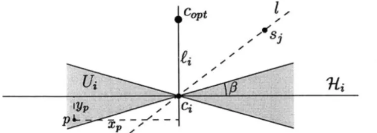
Theorem 2.3.2 For any point-set P C 1Rd, parameters 1 > E, a > 0, y > 0, a random sample R of O(1/(Ela)) points from P spans a flat containing a (1 + E, 1, p + a)-approximate solution for the 1-center with a-outliers for P. Namely, there is a point p G span(R), such that a ball of

radius (1 + e)rcen(P, 1, a) centered at p, contains (1 - a - p) points of P.

Furthermore, we can compute such a cluster in O(f(e,p)nd) time, where

SE p) - 20(l"g E/(3l))

Proof: The proof follows closely the proof of Theorem 4.0.5. Let copt denote the center of the

optimal solution, rot = rcen(P, 1, a) denote its radius, and B opt = Ball(copt, ropt). Let si, ... si

be our random sample, F = span(si, . . . , si)4, and ci = proj(copt, F), and we set 3 =/, and

Ui = {x 1r/2 - # </ZcOptcix < 7r/2 + }

be the complement of the cone of angle 7r - 13 emanating from ci, and having cicopt as its axis.

Let P, = U,

n

P n Bop. For any point p E P, we have

|IpciI x< + yP ropt V1 + 402 = ropt(I + O(E)).

Let

Qi

=

P

\

P. As long as

JQi

;> (a

+ pa)fP, we have a probability of 1/p to sample a

random point that is in

Qi

and is not an outlier. Arguing as in the proof of Theorem 4.0.5, in such a case, the distance of the current flat to c0pt shrank down by a factor of (1 -,2/4). Thus, as

in the proof of Theorem 4.0.5, we perform the random sampling in rounds. In our case, we need

O((1/6) log (1/E)) rounds, and each round requires in expectation 1/P random samples. Thus,

overall, if we sample M = _{O((1/(ep)) log (1/E)) points, we know that with constant probability,}

span(si, . . . , SM) contains a point in distance Eropt from Copt.

As for the algorithm, we observe that using random sampling, we can approximate ropt(P, 1, a) up to a factor of two in o(dn) time. Once we have this approximation, we can generate a set of candidates, as done in Theorem 4.0.7. This would result in

f(E, P) = 0 E0)R . RI 20((1/(t))1092(1A'FPM

candidates. For each candidate we have to spend O(nd) time on checking its quality. Overall, we get

f(e,

p)nd running time. 0 Remark 2.3.3 Theorem 2.3.2 demonstrates the robustness of the sampling approach we use.

Although we might sample outliers into the sample set R, this does not matter, as in our argu-mentation we concentrate only on the points that are sampled correctly. Essentially,

IIFicoptl

is

a monotone decreasing function, and the impact of outliers, is only on the size of the sample we need to take.

Theorem 2.3.4 For any point-set P C Rd, parameters 1 > e, a > 0, p > 0, k > 0, one can compute a (k, a+ p)-center clustering with radius smaller than (1+E) rcen(P, k, a) in 2(k,'4)" n

time. The result is correct with constant probability.

Proof: Let P' be the set of points of P covered by the optimal k-center clustering C, ... , C,

with an outliers. Clearly, if any of the Cis contain less than (P/k)n points of P', we can just skip it altogether.

To apply Theorem 2.3.2, we need to sample O(k/(Eu)) points from each of those clusters (we apply it with p/k for the allowed fraction of outliers). Each such cluster, has size at least

(p/k)n, which implies that a sample of size O(k2

/ (112 )) would contain enough points from Ci.

With constant probability (by the Markov inequality),

IR

c

Cil = Q(k/(Ep)), for i = 1,. . . , k.

We exhaustively enumerate for each point of R to which cluster it belongs. For such partition we apply the algorithm of Theorem 2.3.2. The overall running time is 20((k/(EI) 0(1)))nd.

Chapter 3

The 1-cylinder problem

3.1

Introduction

Let P be a set of n points in Rd. We are interested in finding a line that minimizes the maximum distance from the line to the points. More specifically, we are interesting in finding a (1 + E)-approximation to this problem in polynomial time.

In the following, let Lopt _{denote the axis of the optimal cylinder, rpt denote the radius}

=opt radius(, fot)

= max

I

_[fpt

_-

_p1,

PE P

and Hopt denote the hyperplane perpendicular to ,,Pt that passes through the origin. In this chapter, we prove the following theorem.

Theorem 3.1.1 Given a set of n points in Rd, and a parameter F > 0, we can compute, in nO(lo9(1/6)/e2

) time, a line 1 such that radius(P, 1) ; (1 + e)ropt where ropt is the radius of the minimal 1-cylinder that contains P.

First, observe that we can compute a 2-approximation to the 1-cylinder problem by finding two points p, q E P that are farthest apart and by taking the minimum cylinder having pq as its axis and containing P. It is easy to verify that the radius R of this cylinder is at most 2ropt where ropt is the radius of the minimum cylinder. Let t be a point on the cylinder. The radius of the minimum cylinder that encloses p, q and y, which constitutes a lower bound for ropt, is half the radius of our cylinder. Computing R can be done in O(n2_{d) time.}

up to a factor very close to 1, since we can enumerate all potential values of rpt in the range

R/2, ... , R. The main idea of the algorithm is to compute a (1+ e) distortion embedding of the

n points from Rd into R logn/E2, to guess the solution to the problem there, and then to pull back

the solution to the original space. However, a simple application of this method is known not to work for clustering problems (and the 1-cylinder problem in particular), due to the following difficulties:

1. The optimal solution found in the low-dimensional space does not have to correspond to

any solution in the original space.

2. Even if (1) were true, it would not be clear how to pull back the solution from the low-dimensional one.

To overcome these difficulties, we proceed as follows:

1. In the first step, we find a point h lying on fopt. To be more precise, we guess h by

enumerating polynomially many candidates instead of finding h; moreover, h does not lie

on lopt, but only sufficiently close to it.

2. We remove from P all the points within a distance of (1 + E)ropt from h. Since our final line passes through h, it is sufficient to find a solution for the smaller set P.

3. We embed the whole space into a low-dimensional space, such that, with high probability

for all points p E P, the angle between ph and Copt is approximately preserved.

As we discuss in Steps 3 and 4 of Section 3.1, such an embedding A is guaranteed by the Johnson-Lindenstrauss Lemma.

4. We guess an approximate low-dimensional image Al of the line

1

by exploring polynomially many possibilities. By the properties of the embedding A, we can detect which points in P lie on one side of the hyperplane H passing through h and orthogonal to

1.

We modify the set P by replacing each point p on the other side side of the hyperplane by its reflection around

h.

Note that this operation increases the solution cost only by at most Eropt.

5. It is now sufficient to find an optimal half-line beginning at h, which minimizes the

maxi-mum distance from p E P to the half-line. Moreover, we know that the points are on the same side of a hyperplane that passes through h. This problem can be solved using convex programming tools.

Thus, we use the low-dimensional image of I to discover the "structure" of the optimal solution, namely, which points lie on which side of the hyperplane H. Knowing this structure allows us to reduce our non convex problem to a convex one.

3.2

Computing the approximate 1-cylinder

In this section, we elaborate on each step in computing the cylinder of minimum radius containing a given point set.

Step 1. Finding a point near the line.

Definition 3.2.1 Let U be any set of points in Rd, and E > 0. Let C7-(U) be the convex hull of U. We say that a finite subset A of points is an e-net for U if, for any line f that intersects

C'H(U),

there is a

v

E

A

_{such that dist(v, e)}

_'r2

_t.

Lemma 3.2.2 Let U be a set of points in Rd, and E > 0. We can compute an E-net A(U) for U in (|UI2.5/g)o(IUI) time. The cardinality of

A(U)

is (|U|2.5 o(IUI).

Proof: Let M =

IUI.

Let H be the (M - 1)-dimensional affine subspace spanned by U. Note that

M

<

IU|.

Let

S

C

H

be an ellipsoid such that S/(M + 1)2 C CK(U)

C

8 where

8/(M+

1)2 is

8

_{scaled down around its center by a factor of 1/(M+} 1)2. _{Such an ellipsoid exists,} and can be computed in polynomial time in

IUI,

see [11]. Let B be the minimum bounding box of 8 that is parallel to the main axises of 8. We claim that B/V7 is contained inside 8. Indeed, there exists a linear transformation T that maps 8 to a unit ball S. The point

q = (1/vKAM, 1/V , . .. , 1/VMK _{) lies on the boundary of this sphere. Clearly, T} 1 _{(q) is a corner}

of

3/

_{M, and is on the boundary of 8. In particular,}

diam(B) = v'Mdiam(B/v/1M7) < vIM diam(E)

Figure 3-1: "Helper" points in a convex body after the embedding.

For any line

e,

the same argument works for the projection of those objects in the hyperplane perpendicular to f. Let TPE denote this projection. Then we have

diam(TPt (B)) 5 VM(M + 1)2

diam(TP(U))

K

2VMA(M +

1)2 dist(U,

f).

Next, we partition B into a grid such that each cell is a translated copy of

BE= B/(2iMf-(M +

1)2).

2

This grid has (M2_{-/E)o(M) vertices. Let}

_A(U)

_{denote this set of vertices.}

Let f be any flat intersecting CN(U). We claim that one of the points in A(U) is within distance i dist(U, f) from f. Indeed, let z be any point in CH(U) n f. Let B" be the grid cell containing z, and let v be one of its vertices. Clearly,

dist(v,

e)

11TP(v)TPd(z)l 5 diam(TP(B"))

E 1

diam(TPt(B)) < - dist(U,

£).

2

2xfM(M

+1)2 -2

Thus our assertion is established. U

In order to find the point h, we need to add "helper" points. For each subset S of P with

ISI = O(1/E2), we compute an

E-net

on the interior of the convex body spanned by the points of

S, see Figure 3-1.

4-4-Let A(S) be an E-net for S. Clearly, |A(S)I = (|SJ25/E)O(ISI) where ISI = O(1/e2). We have

IA(S)I

= 20(log(1/)/,

2

)

Lemma 3.2.3 Under the conditions of Lemma 3.2.2, consider the points in G(S) for all sets S. At least one point is at most Eropt away from fopt.

Proof: Project all the points into a hyperplane Hopt that is orthogonal to fopt, and denote

this set of points by P'. Let o be the point of intersection of Lopt with Hopt. Since all the points are at distance at most ropt from topt, all the points projected into H are at distance at most ropt from o. Compute the minimum enclosing ball of the point set P'. It is easy to see that, if the origin of the minimum enclosing ball is not o, then we can come up with a solution for the minimum fitting line of cost lower than ropt by just translating 1 to intersect the center of the ball. Therefore, the minimum enclosing ball of P' has the origin in o.

By Theorem 2.2.3, there exists a set S C P' such that |SI = 0(1/E2), and such that the minimum enclosing ball of the S is at most (E/ 2

)rpt away from o and since the center of any

minimum enclosing ball of a set of points can be written as a convex combination of the points, we conclude that there exists a point p, a convex combination of the points of S such that

D(p, o) < Eropt. Also, distance from p to the closest point of G(S) is at most (E/2)ropt. Therefore,

there exists a point in our E-net that is at most Erpt away from the optimal fitting line. 0 Step 2. Removing the points near h. For simplicity of exposition, from now on, we

assume that h lies on the optimal line fopt. We remove from P all the points within distance

(1 + E)ropt from h.

Clearly, the removal step can be implemented in linear time in the input size. Observe that, after this step, for all points p, the angle between ph and Lopt is in the range [0, r/2 - E/2] U

[7r/2 + E/2, 7] for small enough E. As we will see next, this property implies that the angles do not change in value from less than 7r/2 to greater than 7r/2 after the dimensionality reduction is

applied.

Step 3. Random projection. We show how to find a mapping A: Rd -+ Rd' for d'

-O(log n/e2_{) that preserves all angles}

_ihfope

for p E P up to an additive factor of E/3. For this purpose, we use the Johnson-Lindenstrauss Lemma. It is not difficult to verify (see [8]) that if we set the error parameter of the lemma to E/C for large enough constant C, then all the angles are preserved up to an additive factor of, say, E/4. Hence, for each p E P, the image of p is

on the same side of the image of the hyperplane H as the original points p. Moreover, for any

p

C

P, the angle Z(hp, fopt) is in the range [0, 7r/2 - E/4] U [7r/2 + E/4, r].

Step 4. Guessing the image of 1. We now need to approximate the image Apt where

A is the mapping generated by the Johnson-Lindenstrauss Lemma. For this purpose, we need

to know the direction of 1, since we already know one point through which the line Ahpt passes. Our approach is to enumerate all the different directions of a line Afpt. Obviously, the number of such directions is infinite. However, since we use the line exclusively for the purpose of separating the points p E P according to their angle ZhOpt, and those angles are separated from 7r/2 by

E/4, it is sufficient to find a direction vector that is within angular distance e/4 from the direction

of 1. Thus, it is sufficient to enumerate all directions from an E/4-net for the set of all directions. It is known that such spaces of cardinality nO(1og(1/E)/E2) exist, and are constructible. Thus, we can find the right partition of points in P by enumerating a polynomial number of directions.

After finding the right partition of P, say, into PL and PR, we replace each point in PL by its reflection through h; say the resulting set is P = {2h - p p E P}. Note that there is a

one-to-one correspondence between the 1-cylinder solutions for P that pass through h and the

1-half-line solutions for P' = PL U PR. By definition, the 1-half-line problem is to find a half-line r that has an endpoint at h and minimizes the maximum, over all input points p, of the distance

from p to r. Thus, it remains to solve the 1-half-line problem for P'.

Step 5. Solving the 1-half-line problem using convex programming. We focus on the decision version of this problem. Assume we want to check if there is a solution with cost at most T. For each point p, let C be the cone of all half-lines with endpoints in h and that are within distance T from p. Clearly, Cp is convex. The problem is now to check if an intersection of all cones C, is nonempty. This problem is one in convex programming, and thus can be solved up to arbitrary precision in polynomial time [11].

Chapter 4

k-median clustering

In this chapter, we present an efficient approximation algorithm for the k-median problem.

Definition 4.0.4 For a set P of n points in Rd, let med0pt(P, k) = minKCRdIKI=k ZPEP dist(K, p)

denote the optimal price of the k-median problem, where dist(K,p) = minEK

lixpli.

Let AvgMed(P, k) = med0pt(P, k)/IPI denote the average radius of the k-median clustering.

For any sets A, B C P, we use the notation cost(A, B) = EaEA,bEB

Ijabj|.

If A = {a},

we write cost(a, -) instead of cost({a}, .), similarly for b. Moreover, we define cost(x V y, A) = Esa min (||ax| , I|ayl|).

For a set of points X C Rd, let span(X) denote the affine subspace spanned by the points of

X. We refer to span(X) as the flat spanned by X.

Theorem 4.0.5 Let P be a point-set in Rd, 1 > E > 0, and let X be a random sample of O(1/E3 log 1/E) points from P. Then with constant probability, the following two events happen:

(i) The flat span(X) contains a (1 + E)-approximate 1-median for P, and (ii) X contains a point in distance < 2 AvgMed(P, 1) from the center of the optimal solution.

Proof: Let med₀pt = _{medopt(P, 1) be the price of the optimal 1-median, R = AvgMed(P, 1),}

and let si, . .. , _{su be our random sample. In the following, we are going to partition the random}

sample into rounds: A round continues until we sample a point that has some required property. The first round continues till we encounter a point si, such that | sicopt < 2R, where copt is the center of the optimal 1-median. By the Markov inequality, |Isicop t|| :! 2R, with probability

Figure 4-1: A round terminates as soon as we pick a point outside Ui.

Let's assume that

si

is a sample that just terminated a round, and we start a new sampling

round. Let F be the flat spanned by the first i points in our sample:

si,... , si.

Observe that if

I

IFi

ct

eR, then we are done, as the point proj(c,,t, F) is the required approximation, where

proj(cpt, F) denotes the projection of cpt into Fi.

Note that the distance from cpt to F is monotone decreasing. That is di+1

=

||Fi+1copt|

di

=

|IFic,,pt|. We would next argue that either after taking enough sample points, di is small

enough so that we can stop, or otherwise almost all the points of P lie very close to our spanned

subspace, and we can use P to find our solution.

Indeed, let c1 = proj (c,,t, F), and let

Ui = x Ix E Rd s.t. 7r/2 - 3/3 Z ptci

< ir/2 + 3

l

be the complement of the cone of angle ir

-

#

emanating from ci, and having

cicqp

as its axis,

where /3

e/16. See Figure 4-1. Let 7-4 be the (d

-

1)-dimensional hyperplane passing through

ci and perpendicular to ccpt. For a point p E P, let x, be the distance of p to the line i passing

through cpt and

ci,

and let y, be the distance between p and H-.

If p E Ui, then yp 5 xptan

xp

< 4sinp

43x,

< 5 -pcptIl , as 3 < 1/16. In

cos#3

4

4

particular,

IIpcII

Xp

+

yp

(1 + e/4) ||pcoptIl.

Namely, if we move our center from cot, to

c;,

the error generated by points inside Ui is smaller

than med

0pte/4.

Thus, if the number of points in

Qi

=

P

\

Ui is smaller than ne/4, then we are done. As the

maximum error encountered for a point of

Qi

when moving the center from copt to c, is at most

Thus, it must be that IQj I _{nE/4. We now perform a round of random sampling until we pick} a point that is in

Qj.

Let sj E

Qj

be this sample point, where

j

> i. Clearly, the line 1 connecting

ci to sj must belong to F, as ci E Hi c H. Now, the angle between 1 and fi = line(ci, c0pt) is

smaller than 7r/2 - 3. Namely,

IIopItl|

|copitcII

sin(r/2 - /3)

=|coptci|

|cos3(0)

(1 -

02/4)

Ilcoptci||.

Thus, after each round, the distance between F and cop shrinks by a factor of (1-02/4). Namely, either we are close to the optimal center, or alternatively, we make reasonable progress in each round.

In the first round, we picked a point s, such that ||sucopt| _{2R. Either during our sampling,} we had

I|Fic

₀Pt||

I5

_{eR, or alternatively, we had reduced in each round the distance between our} sample flat and copt by a factor of (1 - /2/4). _{On the other hand, once this distance drops below} ER, we stop, as we had found a point that belongs to Hi and provide a (1 + e)-approximate solution. Furthermore, as long as JQif _{en/4, the probability of success is at least E/4. Thus,} the expected number of samples in a round until we pick a point of

Qj

(and thus terminating the i-th round) is [4/E. The number of rounds we need is

e-log(E/2) '1 2)

M = [logl- ₂/4 log (I - 2/4)

1

0

( log.-).

Let X be the random variable which is the number of random samples till we get M successes. Clearly, E[X] = _{0(1/1E log 1/e). It follows, by the Markov inequality, that with constant}

prob-ability, if we sample 0(1/E _{log(1/c)) points, then those points span a subspace that contains a}

(1 + E)-approximate 1-median center. ₀

We are next interested in solving the k-median problem for a set of points in Rd. We first normalize the point-set.

Lemma 4.0.6 Given a point-set P in Rd, and a parameter k, one can can scale-up space and compute a point-set P', such that: (i) The distance between any two points in P' is at least one. (ii) The optimal k-median cost of the modified data set is at most nb for b = 0(1), where n =| P. (iii) The costs of any k-median solutions in both (old and modified) data sets are the same up to

Proof: Observe that by using Gonzalez [10] 2-approximation algorithm for the k-center

clus-tering, we can compute in

O(nkd)

time a value L (the radius of the approximate k-center clus-tering), such that L/2 < medopt(P, k) < nL.

We cover space by a grid of size LE/(5nd), and snap the points of P to this grid. After scaling, this is the required point-set.

From this point on, we assume that the given point-set is normalized.

Theorem 4.0.7

Let

P be a normalized set of n points in Rd, 1 > E > 0,

and let R be a random

sample of O(i/E log 1/E) points

from

P. Then one can compute, in

0

(d2o(1/E4) log

n)

time, a point-set S(P, R) of cardinality 0 (2O(1/E) log n), such that with constant probability (over the

choice of R), there is a point q E S(P, R) such that cost(q, P) (1 + E)medopt(P, 1).

Proof: Let's assume that we had found a t such that t/2 < AvgMed(P, 1) < t. Clearly, we

can find such a t by checking all possible values of t = 21, for i = 0, ... , O(log n), as P is a

normalized point-set (see Lemma 4.0.6).

Next, by Theorem 4.0.5, we know that with constant probability, there is a point of R with distance < 2 AvgMed(P, 1) 2t from the optimal 1-median center copt of P. Let H = span(R) denote the affine subspace spanned by R. For each point of p E R, we construct a grid Gp(t) of side Et/(10IRI) =

O(tE'

log(1/E)) centered at p on H, and let B(p, 3t) be a ball of radius 2t centered at p. Finally, let S'(p, t) = G,(t) n B(p, 3t). Clearly, if t/2 < AvgMed(P, 1) t, and

IIpcoptI I 2t, then there is a point q E S'(p, t) such that cost(q, P) (1

+

e)med0pt(P, 1). O(log n)

Let S(P, R)

U U

S'(p, 2i). Clearly, S(P, R) is the required point-set, and furthermore,

i=O peR

IS(P,

R)I = 0 (log n)

RI

log) -0 (1/E3 2 _{log n)}

₀

_{(20(1/e4) log n).}

Theorem 4.0.8 For any point-set P C Rd and 0 < E < 1, a (1 + E)-approximate 2-median for P can be found in O(2(1/E)(1) do(1)n logo()1 n) expected time, with high-probability.

Proof: In the following, we assume that the solution is irreducible, i.e., removing a median

creates a solution with cost at least 1

+

Q(E) times the optimal. Otherwise, we can focus on

solving the 1-median instead.

Let c1, c2 be the optimal centers and

P

1

,

P2 be the optimal clusters. Without loss of generality

when compared with the size of P1. In both cases the algorithm returns an approximate solution with constant probability. By exploring both cases in parallel and repeating the computation several times we can achieve an arbitrarily large probability of success.

Case 1:

IP1l

>

IP₂I

> |P1ie. In this case we sample a random set of points R of cardinality

0(1/04 _{log 1/). We now exhaustively check all possible partitions of R into R}

1 = P1 R

and R2 = P2

n

R

(there are 0(20(1/E4 log 1/e)) such possibilities). For the right such

parti-tion,

R,

is a random sample of points in

Pi

of cardinality Q(1/E3 log 1/E) (since

E[IR n

Pi]

-Q(1/E3 _{log 1/c)). By Theorem 4.0.7, we can generate point-sets Si, S2 that with constant}

prob-ability contain c'

E

Si, c' E S

2

, such that cost(ci

V

c, F)

(1

+

)med

0

pt(P, 2). Checking each

such pair c', c' takes

0((nd)

time, and we have

0

(IS_{1 IS21) pairs. Thus the total running time is}

0 (nd20(1/E4 log 1/e) log2

n)

Case

2:

IP1|e > IP2|.

In this case we proceed as follows. First, we sample a set R of A

-0(1/E310g 1/E) points from

P.

This can be done

just

by sampling

A

points from

P,

since with probability 2-0(1/e3 log 1/e) such a sample contains only points from P; we can repeat the whole

algorithm several times to obtain a constant probability of success. Next, using Theorem 4.0.7, we generate a set C1 of candidates to be center points of the cluster P₁. In the following, we

check all possible centers c'

C

C1. With constant probability, there exists c' c C₁ such that

cost(c4, P1) 5 (1 + E/3)cost(ci, P1).

Let (P,, P2) denote optimal 2-median clustering induced by median cl (as above), and let

c' denote the corresponding center of P2. We need to find c' such that cost(c/

V c', P) <

(1

+

_{-/3)cost(cl V c', P) 5 (1 + E)medopt(P, 2). In order to do that, we first remove some}

elements from P1, in order to facilitate random sampling from P2.

First, observe that cost(cl, P2)

5

PJ-

Ic'c'| I

|+ cost(c2, _{P2) and therefore we can focus on the}

case when

IP2|

-

l1c'c'|11

is greater than O(E) -cost(c' V c2,

P),

since otherwise

c'

= c' would be a good enough solution.

We exhaustively search for the value of two parameters (guesses) t, U, such that t/2 <

1|c'1c'2|

K t and

U/2 <

medopt(P, 2)

5 U.

Since

P

is normalized this would require checking

O(log2

n) possible values for t and U. If t > 4U, then t > 4medopt(P, 2) and for any p, q E P we

have ||pqII

K

U. Moreover, for any p E P1, q E P

2

we have

I|pI|

;>

11cc'11

-

|Ic'pII

-

|i4q|II > 2U.

be in P2. The problem is thus solved, as we partitioned the points into the correct clusters, and can compute an approximated 1-median for each one of them directly.

Otherwise, t < 4U and let S = {p

Ijpc|

115 t/4 . Clearly, S C Pl. Moreover, we claim that

IP

>

I

P,

\ S1,

since otherwise we would have

|P2|'c || C 1

and

t

||c'2ct||

cost(c', P1 \ S)

I'

\ S'I

8

Thus,

IIP2'1

Ic'c'I

< 8ecost(c(, P - S) and thus cost(c', P) (1 + 8E)cost(c' V c', P). This

implies that we can solve the problem in this case by solving the 1-median problem on P, thus contradicting our assumption.

Thus,

IP2I

EIP,

\ S1.

We create P'

=

P

\

S = Pj' U P2, where P'

=

PF

\

S. Although P'

might now be considerably smaller than P2', and as such case 1 does not apply directly. We can overcome this by adding enough copies of c' into Pi', so that it would be of size similar to F'.

To carry that out, we again perform an exhaustive enumeration of the possible cardinality of P2 (up to a factor of 2). This requires checking O(log n) possibilities. Let V be the guess for the cardinality of P2, such that V < IP2I < 2V.

We add V copies of c' to Pl'. We can now apply the algorithm for the case when the cardinalities of both clusters are comparable, as long as we ensure that the algorithm reports c' as one of the medians. To this end, it is not difficult to see that by adding copies of c' to Pj' we also ensured that for any 2 medians x and y, replacing at least one of them by c' yields a better solution. Therefore, without loss of generality we can assume that the algorithm described above, when applied to P', reports c' as one of the medians. The complexity of the algorithm is as stated.

Theorem 4.0.9 For any point-set P C Rd, E < 1, and a parameter k, a (1 + E)-approximate k-median

for P

can be

found

in 2(k/)"()

dO(1)n

logO(k) n expected time, with high-probability.

Proof: We only sketch the extension of the algorithm of Theorem 4.0.8 for k > 2. As before,

and exhaustive enumeration of all partitions of the samples into the different clusters, and using Theorem 4.0.7. Thus, we can focus on the case when there is at least one small cluster.

Let Cl,... , _{Ck be the clusters in the optimal solutions, with corresponding centers cl,... , ck.}

Let C, .. . , _{C, be the heavy clusters, and let C±i+ be a small cluster, such that its center cj+1 is} the closest one to ci, ... , ci.

We use an argument, similar to the argument used in Theorem 4.0.8, to show that we can shrink C1,... , Ci to make their sizes comparable to Ci+₁

-" Let AvgMed = AvgMed(Ci U ... U C, i). If the distance from any cj,

j

> i to the nearest ci, . . . , ci is less than t < AvgMed < 2t, then we can remove all such medians cj without

incurring much cost, as

1C1

nE/k.

" Otherwise, this means the medians cj,

j

> i, are at least at distance AvgMed /2 from

c,... ,Ci.

" On the other hand, cj+1 cannot be too far from ci,... , ci, because then we could easily

separate the points of C1, ... , Ci from the points of Ci+1, ... , Ck.

* Thus, we can "guess" (i.e., enumerate O(log n) possibilities), up to a factor of two, the distance between cj+1 and its closest neighbor in ci, ... , ci. Let t be this guess.

" We can assume that all points within distance < t/2 to ci,... ,ci belong to clusters

Ci,... , _{Ci, and focus on clustering the remaining set of points.}

" The number of points with distance > t/2 from ci,... , Ck is comparable to the size of Cj+i.

Thus we can proceed with sampling.

This yields a recursive algorithm that gets rid of one cluster in each recursive call. It performs

2(k/E)0(1) log0

~')

n recursive calls in each node, and the recursion depth is k. Thus, the algorithm

has the running time stated. Note that we need to rerun this algorithm

0

(20(k) log n) times to

Chapter 5

Smaller Core-Sets for Balls

5.1

Introduction

Given a set of points P C Rd and value e > 0, a core-set S C P has the property that the smallest ball containing S is within e of the smallest ball containing P. That is, if the smallest ball containing S is expanded by 1 + c, then the expanded ball contains P. It is a surprising fact that for any given E there is a core-set whose size is independent of d, depending only on E. This is was shown by Badoiu et al.[6], where applications to clustering were found, and the results

have been extended to k-flat clustering. [13].

While the previous result was that a core-set has size O(1/2), where the constant hidden in the 0-notation was at least 64, here we show that there are core-sets of size at most 2/E. This is not so far from a lower bound of 1/c, which is easily shown by considering a regular simplex in 1/c dimensions. Such a bound is of particular interest for k-center clustering, where the core-set size appears as an exponent in the running time.

Our proof is a simple effective construction. We also give a simple algorithm for computing smallest balls, that looks something like gradient descent; this algorithm serves to prove a core-set bound, and can also be used to prove a somewhat better core-core-set bound for k-flats. Also, by combining this algorithm with the construction of the core-sets, we can compute a 1-center in

time O(dn/c + (1/c)").

In the next section, we prove the core-set bound for 1-centers, and then describe the gradient-descent algorithm.

5.2

Core-sets for 1-centers

Given a bali B, let CB and rB denote its center and radius, respectively. Let B(P) denote the

1-center of P, the smallest ball containing it. We restate the following lemma, proved in

[9]:

Lemma 5.2.1 If B(P) is the minimum enclosing ball of P C R d, then any closed half-space

that contains the center cB(p) also contains a point of P that is at distance rB(P) fTom CB(P)-Theorem 5.2.2 There exists a set S C P of size at most 2/c such that the distance between CB(S) and any point p of P is at most (1 +

E)rB(P)-Proof: We proceed in the same manner as in [6]: we start with an arbitrary point p E P and set So = {p}. Let ri TrB(Si) and ci cB(Si). Take the point q E P which is furthest away from

ci and add it to the set:

Si+1

+- Si

Uj{q}.

Repeat this step 2/E times. It is enough to show that the maximum distance from one of the centers ci to the points of P is at most R.

Let c cB(P), R rB(P), R (1

+ E)R, A

ri/R, di

f|c

-

cilI

and

Ki

= |ci+1 -

cilI.

Since the radius of the minimum enclosing ball is R, there is at least one point q E P such that

I

Iq

- ci I I > R. If Ki = 0 then we are done, since the maximum distance from ci to any point is at

most R. If Ki > _{0, let H be the hyperplane that contains ci and is orthogonal to (ci, ci+i). Let} H+ be the closed half-space bounded by H that does not contain c±is. By Lemma 6.3.1, there must be a point p

E

Si fH+

such that

IIci

- p|| =

ri

=

A

2

R,

and so

|Ic±is

-

p1

/Ai R

2

+ Ki.

Therefore,

Ai+R

>

max(R

- Ki,

A2R 2

+ K2) (5.1)

We want a lower bound on Aj+i that depends only on A₂. Observe that the bound on Aj+1 is smallest with respect to Ki when

R - Kj

= A 2R 2 + K

R2

-

2KR

+K

= A

R

2 ₊

_K

(1

- A2)R

Ki =

Using (5.1) we get that

R

(1-,2)R

A+R

2 t 2 i (5.2)

Substituting -yj = in the recurrence (5.2), we get 7j+1 = -1i = yi(1+ W+ -Y..)

-7i

+

1/ 2. Since Ao = 0, we have yo= 1,so y 1

+

i/2 andAi2 1-

Ti

1/2an A > 1±/ hat is, to get

Ai > 1 - c, it's enough that 1 +

i/2

1/E, or enough that i > 2/E.

5.3

Simple algorithm for 1-center

The algorithm is the following: start with an arbitrary point ci E P. Repeat the following step

1/62 times: at step i find the point p E P farthest away from ci, and move toward p as follows: ci+1 <- ci

+

(p - ci)+.

Claim 5.3.1 If B(P) is the 1-center of P with center cB(p) and radius rB(P), then cB(P) -CiII rB(P)/VZ7 for all i.

Proof: Proof by induction: Let c CB(P). Since we pick ci from P, we have that ||c - c1 < R = rB(P). Assume that Ic - ci I R/7. If c = ci then in step i we move away from c by at most R/(i

+

1) R/ i

+

1, so in that case

Ic

- cj+1 I R/vi

+

1. Otherwise, let H be

the hyperplane orthogonal to (c, ci) which contains c. Let H+ be the closed half-space bounded

by H that does not contain ci and let H- = R \ H+. Note that the furthest point from ci in

B(P)

f

H- is at distance less than

Ii|cI

- cj2 + R2 _{and we can conclude that for every point}

q P fH-, I ci - qjI < VA|ci -

cu|

2 + R2. By Lemma 6.3.1 there exists a point q

C

P fH+

such that IIci - qf I I I c - c |2 + R2. This implies that p E P fH+. We have two cases to consider:

" if cj+1 E H+, by moving ci towards c we only increase

I|c±i+

- clI, and as noted before if

ci = cwe have iici+1 -ci < R/(i+ 1) R/ i+1. Thus, 1ici+1 -ci < R//i±+ 1

" if cj+1 E H-, by moving ci as far away from c and p on the sphere as close as possible to

H-~, we only increase IIc±i+ - cii. But in this case, (c, ci+1) is orthogonal to (ci, p) and we have lci I-cl = / = R/

+

1.

Chapter 6

Optimal Core-Sets for Balls

6.1

Introduction

In the previous chapter we showed that there are core-sets of size at most 2/E, but the worst-case lower bound, easily shown by considering regular simplices, is only [1/c ].[4] In this chapter we show that the lower bound is tight: there are always E-core-sets of size [1/c]. A key lemma in the proof of the upper bound is the fact that the bound for L6wner-John ellipsoid pairs is tight for simplices.

The existence proof for these optimal core-sets is an algorithm that repeatedly tries to improve an existing core-set by local improvement: given S C _{P of size k, it tries to swap a point out of S,} and another in from P, to improve the approximation made by S. Our proof shows that a

1/k-approximate ball can be produced by this procedure. (That is, if the smallest ball containing the output set is expanded by 1 + 1/k, the resulting ball contains the whole set.) While it is possible to bound the number of iterations of the procedure for a slightly sub-optimal bound, such as 1/(k - _{1), no such bound was found for the optimal case. However, we give experimental evidence} that for random pointsets, the algorithm makes no change at all in the core-sets produced by the authors' previous procedure, whose guaranteed accuracy is only 2/k. That is, the algorithm given here serves as a fast way of verifying that the approximation E is 1/k, and not just 2/k.

We also consider an alternative local improvement procedure, with no performance guar-antees, that gives a better approximation accuracy, at the cost of considerably longer running time.