Effects of green building certification on organizational productivity metrics

Publisher’s version / Version de l'éditeur:

Vous avez des questions? Nous pouvons vous aider. Pour communiquer directement avec un auteur, consultez la première page de la revue dans laquelle son article a été publié afin de trouver ses coordonnées. Si vous n’arrivez pas à les repérer, communiquez avec nous à PublicationsArchive-ArchivesPublications@nrc-cnrc.gc.ca.

Questions? Contact the NRC Publications Archive team at

PublicationsArchive-ArchivesPublications@nrc-cnrc.gc.ca. If you wish to email the authors directly, please see the first page of the publication for their contact information.

https://publications-cnrc.canada.ca/fra/droits

L’accès à ce site Web et l’utilisation de son contenu sont assujettis aux conditions présentées dans le site

LISEZ CES CONDITIONS ATTENTIVEMENT AVANT D’UTILISER CE SITE WEB.

Research Report (National Research Council of Canada. Construction),

2017-03-29

READ THESE TERMS AND CONDITIONS CAREFULLY BEFORE USING THIS WEBSITE. https://nrc-publications.canada.ca/eng/copyright

NRC Publications Archive Record / Notice des Archives des publications du CNRC : https://nrc-publications.canada.ca/eng/view/object/?id=9cae7920-03d1-459e-ab14-2fef54016a92 https://publications-cnrc.canada.ca/fra/voir/objet/?id=9cae7920-03d1-459e-ab14-2fef54016a92

NRC Publications Archive

Archives des publications du CNRC

For the publisher’s version, please access the DOI link below./ Pour consulter la version de l’éditeur, utilisez le lien DOI ci-dessous.

https://doi.org/10.4224/23001861

Access and use of this website and the material on it are subject to the Terms and Conditions set forth at

Effects of green building certification on organizational productivity

metrics

1

Effects of Green Building Certification on

Organizational Productivity Metrics

Guy R. Newsham, Jennifer A. Veitch, Vera Hu

Construction Portfolio, National Research Council of Canada (NRC)

1200 Montreal Rd., Building M24, Ottawa, Ontario, K1A 0R6, Canada guy.newsham@nrc-cnrc.gc.ca

NRC Construction Research Report RR-399 (NRC-CONST-56186)

2

Effect of Green Building Certification on Organizational Productivity

Metrics

Abstract

There is increasing interest in understanding how office accommodation affects organizational productivity. Data on metrics of engagement, job satisfaction, job performance, and facility complaints for thousands of employees of a large Canadian financial organization were analysed to explore differences in

outcomes between those working in green-certified office buildings and those in otherwise similar conventional buildings. Overall, green-certified buildings demonstrated higher scores on survey outcomes related to job satisfaction, value to clients and stakeholders, evaluation of management, and corporate

engagement. There was also a tendency for manager-assessed job performance to be higher in green-certified buildings. Nevertheless, not all green-certified buildings outperformed all conventional buildings, and superior performance was not exhibited on all outcomes examined. A key observation is that such metrics are routinely recorded by organizations, but relating them to building

characteristics is new. Recognition of such data sets opens up many promising avenues for buildings research.

Keywords: green buildings, commercial offices, productivity, sustainable design, job performance, job satisfaction

Introduction

Background

There has been a long history of research establishing linkages between the physical office environment and the comfort and satisfaction of occupants [e.g. Brill et al., 1984; Sundstrom, 1986]. People in positions of influence who demand economic indicators to inform decisions on office accommodation and environmental control choices have often sought information on effects beyond indoor environment comfort; i.e. metrics perceived to have a more direct effect on employee health and well-being, and organizational productivity. Organizational productivity, in its most straightforward definition, is the ratio between the value of an organization’s outputs and the cost of its inputs. Real estate may affect organizational productivity on the cost side of the

3

ability to do their work, the quality of their work, and their opinion of, and loyalty to, their employer. Such information is now growing in importance as enlightened employers seek sustainability options for their real-estate portfolios that go beyond energy efficiency.

The largest expenses for most white-collar organizations are staff (salaries, benefits etc.), buildings (leases, maintenance etc.), and information technology. An analysis of how the second category affects the first seems like an obvious activity in the context of financial due-diligence and budget allocation choice, but is rarely undertaken. In part this is because the information for these analyses rests in different parts of organizations – human resources (HR) owns employee data, and facilities managers (FM) or corporate real estate departments have building data.

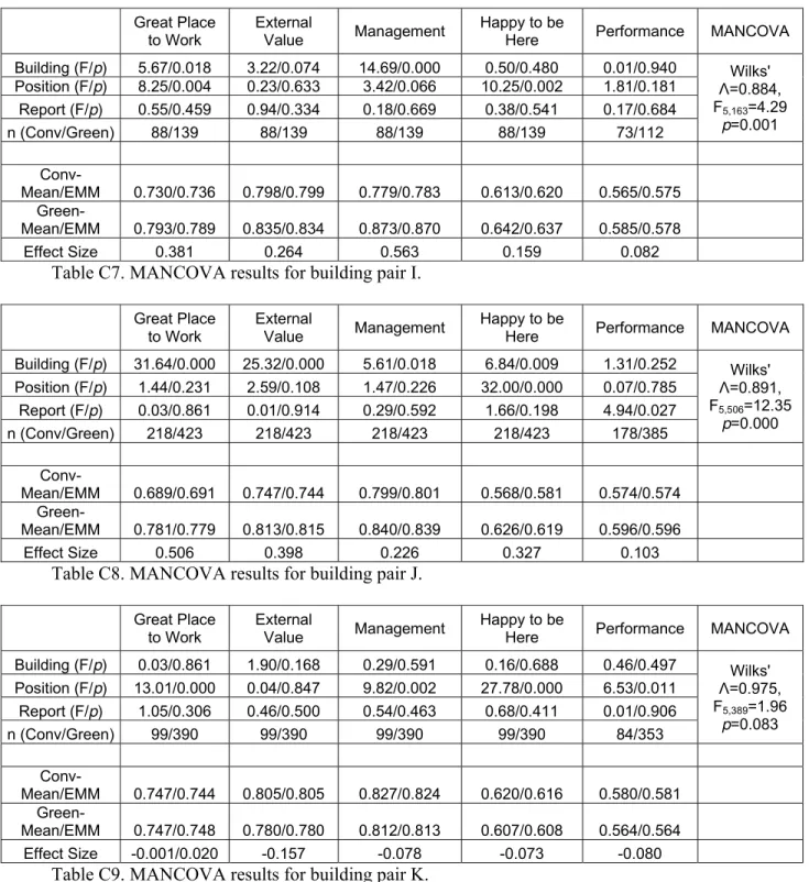
Although these are the top expense categories, the cost of staff typically dwarfs the cost of buildings. Figure 1 illustrates a widely-cited breakdown of the costs

associated with office workplace costs over a 10-year period [Brill et al., 2001]. Another common rule of thumb that is often quoted is that the annual operational costs of an office space are, on average $300/ft2 for staff payroll, $30/ft2 for space rent, and $3/ft2 for utilities [e.g. Best, 2014]. Thus, one would not want cost savings in buildings to come at the expense of staff’s ability to do their work. Ideally an organization would identify building strategies that support the productivity of the organization, and are cost-effective as a whole. In other words, a relatively small investment in building design and operation can have a relatively big benefit on organizational productivity through positive effects on staff (and energy use).

Figure 1. The costs associated with office workplace costs over a 10-year period [Brill et al., 2001].

Good quality studies demonstrating linkages between building characteristics and organizational productivity are rare. This is partly because there has been no broadly accepted definition of what constitutes appropriate metrics, and thus suitable datasets have not been generated. At one time decision-makers sought very simple cause-and-effect relationships; i.e. ‘If <BUILDING FEATURE X> is replaced with <BUILDING FEATURE Y> then productivity will increase by Z%’. This is partly a hangover from an industrial production line model of productivity in terms of the output of standard, directly countable units.

There is increasing acceptance that such a model is not applicable to most white-collar workplaces, where output is rarely measured in such terms. Instead, productivity

4

in white-collar workplaces is better represented by a basket of metrics, sometimes measured in different units, that all influence the overall productivity equation in an organization. This is the efficiency definition of organizational productivity [Pritchard, 1992]. Not all metrics can be defined in currency (or other common) units, and the relative value of each metric varies between industries and countries. This is a more complex and nuanced approach, but offers a realistic pathway to move forward in this domain that an overly simple metric does not offer. Furthermore, organizations are now familiar with the use of multi-metric (or “balanced scorecard”) approaches in other domains [Kaplan & Norton, 1992].

Two important industry publications have appeared recently that map out an approach to valuing better buildings with respect to organizational productivity using multiple metrics. The CABA White Paper “Improving Organizational Productivity with Building Automation Systems” proposed one such scorecard structure [Thompson et al., 2014, Table 1], inspired by food nutrition labels. Metrics included concepts related to: environmental satisfaction, job satisfaction, health, staff commitment, absenteeism, business unit performance, environmental conditions, energy use, and responsiveness to facility complaints. The choice of these metrics was not arbitrary; they were derived from a conceptual model of the interplay of workplace environment elements, employee effects and behaviours, and organizational outcomes established by a logical connecting of multiple studies addressing pieces of the model, as shown in Figure 2. No single study has ever measured this end-to-end network of variables and demonstrated their interaction.

Figur envir produ Well (Ed.) build to su simp in ide envir and p re 2. One po ronment in uctivity (fro The Wor lbeing and P ), 2014] pro dings on org upport a bus ple payback entifying ou ronment, in physical me ossible deta an office bu om Thomps rld Green B Productivity ovided an in ganizational iness case f on energy s utcomes tha cluding: HR easures of th ailed concep uilding coul son et al. [20 Building Cou y in Offices nternationall l productivit for green bu savings. Th at could be p R outcomes he indoor en 5 ptual model ld affect job 014]). uncil (WGB : The Next ly-agreed fr ty metrics. uilding1 prin he WGBC re positively a , workplace nvironment. showing ho b satisfactio BC) in their Chapter for ramework fo This report nciples and eport also to affected by e e perception . ow element n and organ publication r Green Bui or evaluatin was motiva certification ook a multi-enhancemen n, complaint ts of the phy nizational n “Health, lding” [Alk ng the effect ated by a de n beyond a -metric appr nts to the bu ts to the FM ysical ker t of esire roach uilt M,

6

A key insight from the WGBC report was the recognition that data on many of these important metrics already exist in an organization and are collected routinely. In other words, one does not necessarily have to engage in an expensive or invasive data collection campaign to explore the relationship between the built environment and organizational productivity in a given organization; rather, it may be a matter of securing permission to use existing data sources for this purpose, collating them, parsing them by building, and associating them with local building characteristics.

For example, HR databases might already hold data pertaining to staff

retention/turnover, absenteeism, and other aspects of employee health and well-being. The HR departments in many organizations also conduct regular employee opinion surveys that contain data on job satisfaction and organizational commitment. The marketing departments in large organizations might conduct customer satisfaction surveys, and the finance department will likely have data on business unit performance. Many office building landlords regularly administer tenant satisfaction surveys that contain items related to environmental satisfaction. The FM company (frequently a separate entity from the tenant and landlord) often maintains a database of complaints about the built environment registered by individuals, as well as the response time and cost. The FM might also keep historical records from the building automation system, which will provide data on some physical indoor environment conditions, such as space temperature and humidity, and zone-level CO2 concentration.

This paper reports on analysis of a sub-set of such multi-metric data from one large private-sector Canadian financial organization. At the time of the analysis some of the major office buildings occupied by the study organization had been green-certified, and the analysis addressed the hypothesis that metrics related to organizational

productivity were improved in green-certified buildings, compared to otherwise similar conventional buildings. This hypothesis is promulgated by national green building organizations (e.g. USGBC and CaGBC), and has been supported by some [e.g. Newsham et al, 2013; Frontczak et al, 2012], but not all [e.g. Gou et al, 2011; Thatcher & Milner, 2012], published field research. This study represents an early

implementation of the proposed CABA/WGBC multi-metric approach to this hypothesis.

Method

Data preparation and cleaning

This study was an analysis of archival data from the study organization’s records. Data files provided by the corporate real estate group and the HR group were merged. Data confidentiality was of utmost importance. To prevent identification of individuals, all employee information was anonymized before it was delivered to the research team. Employee names were replaced by a unique, but meaningless, ID code that allowed data in multiple files to be linked, and applicable demographic

characteristics were categorized.

The data from the corporate real estate group included building characteristics (e.g. age, size, location, lease), Green/LEED credits for applicable major office

buildings, work order history (i.e. complaints to the FM), and a mapping of employees to buildings.

7

The data from the HR group included employee demographics (e.g. age, gender, education, dependents, languages), job classifications, salaries and other financial compensation, staffing actions (e.g. hires, departures), manager-assessed performance ratings, and responses to the corporate Employee Opinion Survey (EOS). The EOS is a survey containing over 100 items that the organization administers annually to all staff. The data received were composite scores on 16 scales created by the study organization from responses on the 100 items. The exact mapping of individual survey items to these 16 variables, and the method by which this was done, was not shared with the research team because it was proprietary to the external survey administrator engaged by the financial organization.

From the full set of data files two master files were created containing the subset of variables that were judged to be the most useful for the analysis goals. The first master data file collated information on the characteristics of each building, and the second master data file collated the information on each employee. An employee mapping file showed to which building each employee was assigned as their ‘home’ workplace in August 2015. These master files contained approximately 120 million data points.

Data were received up to September 2015, and this analysis focussed on data from the 2014-15 period, which may be termed the ‘2015 dataset’ in shorthand. This choice was made primarily because it included the only point in time for which a direct and straightforward mapping of employees to buildings was available.

Nevertheless, even within this time period different datasets were separated in time, creating some unavoidable ambiguity or noise in the data. For example, the employee mapping came from August 2015, the Employee Opinion Survey (EOS) data came from February 2015, and the manager-assessed performance data from the nearest point in time came from November 2014. The implicit assumption was that an

employee in a given building in August 2015 was in the same building when they answered the EOS, and when their performance was assessed by their manager. This might not have been the case, although movement between ‘home’ buildings was thought to be relatively small over this timeframe2.

In total, 70,958 employees were mapped to the study organization’s 1,640 North American buildings. Of these, 70 buildings were classified as ‘major’ office buildings with 40,573 employees. The data set was narrowed down further to office buildings with >100 employees in the mapping file. This yielded 46 buildings.

Outcome measures

Employee opinions and manager-assessed performance were the focus of both building-level and individual analyses. FM complaints about HVAC issues per

employee at the building level were also examined. The employee opinion variables in these analyses were derived by the research team from the 16 EOS scales that had been provided. After preliminary analyses, it was judged that a further grouping of the 16 EOS scales would create more reliable outcomes and aid in interpretation of results. Principal Components Analysis (PCA) with Varimax rotation was used as an aid to developing a smaller set of composite variables, although the process was also guided by thematic linking based on the wording of individual items. The final mapping of the 16 initial variables to four higher-level composites is shown in Table 1. ‘Great Place to Work’ is related to employee job satisfaction and corporate engagement. ‘External Value’ is related to how the organization interacts with the outside world.

8

they report to. ‘Happy to be Here’ relates to whether an employee’s expectation of their job was fulfilled, and their desire to remain with the organization over a longer time period. The composite scales were means of the individual scales that made up the composite. They all had a numerical value from 0-1, with a higher value indicating a more favourable opinion. The internal consistency (as indicated by Cronbach’s alpha) of the first three composites was very good, whereas it was poor for the ‘Happy to be Here’ composite. Nevertheless, this composite was maintained because of the face validity of linking the items, and the undesirable option of using individual scales given the uncertainty of how the individual survey items mapped to the scales.

Engagement

EOS_Great Place to Work (α = 0.94)

Collaboration Enablement Talent Management Engagement Cluster Recognition and Rewards

Citizenship

EOS_External Value (α = 0.86) Competitiveness

Client Focus Vision Values Direction Confidence in the Future

Immediate Manager

EOS_Management (α = 0.92) Leadership

Performance Management

Employee Expectation EOS_Happy to be Here

(α = 0.38) Retention

Table 1. Mapping of 16 initial EOS variables to the four composite variables used in the analyses. Scale reliability and internal consistency is indicated by Cronbach’s alpha.

Each employee had a performance assessment rating from their manager, made using a five-point scale. This scale was translated into a numerical value from 0-1, with a higher value indicating better assessed performance, consistent with the EOS scale (see Table 2).

Code Description Numerical Value

G1 Exceptional 1.00

G2 Outstanding 0.75

G3 High Performance 0.50

G4 Lower Performance 0.25

G5 Poor Fit 0.00

Table 2. Mapping of manager-assessed performance rating scale to the numerical value used in the analyses.

For FM complaints, the focus was on the subset of complaint types recorded in the data file that were associated with the HVAC system (see Table 3). This was the category of complaints judged to be most likely to be affected by green building practices3. The total number of complaints allocated to all four of these sub-categories, divided by the number occupants, was used as the performance metric.

9

Complaint Description HVAC – Leak HVAC – Repairs HVAC – Too Hot/Too Cold General Smell/Odour in Air

Table 3. The four complaint categories from the FM complaints file that were summed to provide a total HVAC complaints metric used in the analyses.

Independent Variable: Building Type

Of the 46 buildings selected for analysis there were 13 buildings that had been LEED-certified (at some level) as of August 2015. This criterion was chosen because the research team could be sure that all green building features had been implemented and validated. The remaining 33 buildings formed the conventional buildings sub-set, although some of these were pending green certification at the time. For each green-certified building a matched conventional building was sought, and buildings pending green certification were excluded from the matching process; conventional buildings that were not matched to a green building (N=23) were dropped from further

consideration in this analysis. The initial matching choices were based on building location (and thus similar regional conditions and climate), building age (of original construction date, not most recent renovation), and size.

Unfortunately, it was not possible to find an appropriately-matched conventional building for every green-certified building. Of the 13 green-certified buildings only 10 could be matched with a conventional building, so the final dataset for analysis consisted of 10 matched pairs, with a sample totalling 20 buildings and 14,569

individual employees. The sample is described in Table 4, where the matched pairs are shown together; similar information for the larger office buildings not used in the analysis is shown in Appendix A. In some cases the host organization occupied the entire building, in other cases a “building” refers to the floors occupied by the study organization within a large building. Nevertheless, each “Building ID” in Table 4 refers to a unique address.

After the initial matching based on building location, age and size, a check was conducted to ensure that other building characteristics, including those of the occupants, were similar at the building average level (see Table 4). Of course, all buildings were matched on employer, an important similarity criterion that is implicit in this study, but which has not been the case in other green buildings research. Matching among a relatively small population of buildings from a single portfolio, especially from a building type as relatively heterogeneous as large office buildings, can never be perfect. Nevertheless, this two stage process yielded what the research team judged to be an acceptable set of matched pairs.

10

Building Characteristics Characteristics of Employees in each Building

Pai r I D B u ild ing ID G ree n Bu ild in g Re g ion Total Are a O c c u pi e d by Stu d y O rgan iz ation R a ng e ( ft 2 ) Nu m b e r of Employ ee s Ma p ped to Build ing Ra nge Dens ity C o n s tructio n Da te Gender Ag e Degre e Commut e ( k m) Depen d e n t Total Pay (lo c al $) Positio n Re p o rt FTPT Tenur e (y rs ) Actio n A A1 0 Northeast US >500,000 1,001-5,000 3.39 1981-1990 0.79 38.5 3.6 14.5 2.6 260,828 5.9 2.5 1.00 4.5 0.9 A2 1 Northeast US 200,001-500,000 501-1,000 3.45 After 2000 0.67 42.0 3.4 33.3 2.5 155,854 5.3 2.8 1.00 5.0 1.1 B B1 0 Western Canada <50,001 101-500 4.75 1971-1980 0.57 42.5 2.9 12.0 2.4 72,518 4.3 3.0 0.99 7.9 0.7 B2 1 Western Canada <50,001 101-500 3.06 1991-2000 0.75 37.8 3.2 10.9 2.3 116,000 5.5 2.4 0.98 6.1 0.8 D D1 0 Southern Ontario 50,001-100,000 101-500 3.92 1971-1980 0.57 42.6 3.0 14.2 2.2 66,414 4.3 1.4 0.98 7.4 0.9 D2 1 Southern Ontario <50,001 101-500 4.49 1971-1980 0.42 40.5 3.0 14.6 2.4 58,473 4.0 1.3 0.95 8.0 1.2

E E1 0 Southern Ontario 200,001-500,000 1,001-5,000 4.05 Before 1971 0.46 42.0 3.0 31.6 2.3 59,159 4.0 7.0 0.89 8.2 1.0

E2 1 Quebec 200,001-500,000 1,001-5,000 5.38 Before 1971 0.35 43.9 2.9 18.2 2.2 53,523 3.7 3.6 0.90 9.3 1.3

F F1 0 Western Canada 50,001-100,000 101-500 5.70 1981-1990 0.59 39.6 3.0 10.7 2.2 79,268 4.6 5.4 0.97 7.3 0.9

F2 1 Western Canada 50,001-100,000 101-500 4.62 1981-1990 0.52 42.2 3.0 11.7 2.4 68,265 4.6 3.7 0.99 8.0 0.8

G G1 0 Southern Ontario 200,001-500,000 1,001-5,000 6.24 1981-1990 0.65 44.6 2.9 38.2 2.4 94,548 5.3 4.8 0.99 8.3 0.8

G2 1 Southern Ontario >500,000 1,001-5,000 4.75 1971-1980 0.55 41.1 3.4 19.7 2.3 98,194 5.3 21.1 0.98 7.5 0.9

I I1 0 Western Canada <50,001 101-500 4.06 Before 1971 0.52 42.4 2.9 10.1 2.4 59,741 4.2 2.9 0.96 8.9 0.9

I2 1 Western Canada 50,001-100,000 101-500 3.00 Before 1971 0.48 43.1 2.9 12.2 2.3 66,978 4.6 15.5 0.89 9.2 1.1

J J1 0 Western Canada <50,001 101-500 5.28 Before 1971 0.37 46.2 2.7 14.7 2.1 57,185 3.5 2.4 0.81 11.1 1.3

J2 1 Western Canada 100,001-200,000 501-1,000 3.79 1971-1980 0.38 44.5 3.0 18.9 2.1 63,733 4.2 9.3 0.89 9.4 0.9

K K1 0 Western Canada <50,001 101-500 2.61 1971-1980 0.35 44.5 3.1 17.9 2.1 78,535 4.7 7.5 0.90 9.1 1.0

K2 1 Western Canada 100,001-200,000 501-1,000 3.67 Before 1971 0.38 44.2 3.0 17.2 2.1 70,786 4.4 6.8 0.89 8.6 1.0

L L1 0 Southern Ontario 200,000-100,001 101-500 2.61 1981-1990 0.83 41.9 2.7 41.2 2.4 77,784 4.7 2.2 1.00 8.3 0.8

L2 1 Southern Ontario 50,001-100,000 501-1,000 8.87 1981-1990 0.33 44.3 2.9 32.3 2.3 58,414 3.9 2.9 0.97 8.8 1.2

Table 4. Characteristics of the paired buildings used in the analyses; shading indicates the green-certified building in a matched pair. Density=mapped employees/1000 ft2; Gender=”"mean” gender (female=0, male=1) of employees in the building; Age=mean age of occupants;

Degree=mean level of education reached (e.g. 3= Bachelor’s Degree); Commute=median commuting distance; Dependent=mean number of dependents in occupants’ families; Total Pay=median annual compensation; Position=mean position in hierarchy (higher value indicates higher position); Report=mean number of direct and indirect reports; FTPT=mean ratio of full-time to part-time employees (0=all part-time, 1=all full-time);

11

Statistical models

Two approaches to the data analysis were taken: examining differences at both the building level between matched pairs, and at the level of individual employees between buildings in matched pairs.

At the building level, the outcome measures were the building average scores on the four EOS scales, manager-assessed performance, and FM complaints. For example, if a building had 500 employees who responded to the EOS, then for a particular EOS metric the average of the 500 responses was taken as the value that represented performance at the building average level. The approach taken had been successfully applied in an earlier green building study [Newsham et al, 2013]. In that study, matched pairs of buildings were recruited that were as similar as possible in respects other than green certification, and then tested for statistical significance of differences in outcomes between the set of building pairs using the non-parametric Wilcoxon Signed Ranks Test. This test is recommended when the sample size is relatively small and when there is no prior expectation that the data are normally distributed [Siegel & Castellan, 1988]. Moschandreas & Nuanual [2008] also used this approach for their green building study.

As a further step, a multi-variate analysis of variance with covariates (MANCOVA) using individual employee data was conducted separately for each matched pair of buildings. MANCOVA assumes that the individual outcomes scores in each building are normally distributed. With the building-level analysis the matching process implicitly controlled for factors other than the ‘green-ness’ of the buildings. With MANCOVA on a building pair, data at the individual employee level was used to explicitly statistically control for differences in the characteristics of individuals4 in the two building populations using covariates. The result then indicates, for a given

building pair, whether there was a difference in each outcome variable associated with the fact that one of the buildings was green. Repeating this process across all pairs may reveal a pattern of results that reinforces (or not) the analysis with building-level data.

The choice of covariates was directed at a reasonable sub-set of variables, with limited inter-correlation between themselves, that displayed some differences between building pairs even after matching. Thus, the difference in the covariates might be expected to explain some of the difference in outcomes between the building pairs. Covariates that would be good choices across all building pairs were desirable, to result in a consistent model specification. Gender and age are common choices for covariates in data coming from humans. However, in this case Table 4 shows that the matching process already led to building pairs with, in general, very similar occupant average age and gender balance. Therefore, Position and Reports were chosen (defined in Table 4) as covariates, as these might suggest differences in management hierarchy between buildings, which might be expected to influence these outcomes5.

Consistent with good practice in this domain, the starting point was a MANCOVA analysis on all six outcomes. If that revealed a statistically-significant overall effect, the univariate ANCOVAs were interpreted for each outcome separately.

Results and discussion

In interpreting these results, trends in the pattern of statistical tests across all outcomes, and across many tests and using several different statistical techniques, were

12

examined to avoid giving undue weight to any one outcome. Several factors had increased noise in the data or reduced the statistical power of the analyses, such as the possibility of some EOS data and performance ratings having been measured while the employee occupied a different building, and it could not be ruled out that some

buildings categorized as conventional nonetheless had some features of a green building. Therefore, this work should be considered exploratory, with consideration given to tests with a p-value <0.1 (more liberal than the standard 0.05) as potential contributors to larger trends. However, emphasis is placed only where several such tests reinforce each other and where they are consistent with prior research. Common effect size metrics were used to judge the practical importance of statistically-significant effects.

Analysis at the building average level

Table 5 shows the mean scores for each outcome for each building in the matched pairs; similar information for the larger office buildings not used in the analysis is shown in Appendix B. First, it is apparent that most building-level EOS scores were above 0.6 (on a scale from 0-1), suggesting that study organization employees on average were generally satisfied with their jobs.

The Wilcoxon test takes two aspects of these data into account in determining statistical significance of the overall effect: the number of pairs in which the difference in means between the buildings in the pair favour one building type; and the relative size of the differences

13 Building Info EOS_ Great Place to Work EOS_ External Value EOS_ Management EOS_ Happy to be Here Manager-assessed Performance Pair ID Building ID Gr een B u ild in g

mean sd mean sd mean sd mean sd EOS_

n mean sd n _HVAC Com p laints To tal Com p laints A A1 0 0.694 0.184 0.736 0.169 0.767 0.187 0.579 0.197 1247 0.650 0.175 217 NA NA A2 1 0.711 0.184 0.750 0.167 0.775 0.191 0.548 0.190 504 0.628 0.188 519 NA NA B B1 0 0.725 0.180 0.778 0.153 0.769 0.206 0.628 0.208 137 0.509 0.112 85 4 105 B2 1 0.738 0.141 0.776 0.133 0.782 0.161 0.622 0.156 95 0.592 0.190 19 8 82 D D1 0 0.761 0.174 0.817 0.158 0.800 0.182 0.610 0.167 152 0.539 0.181 103 1 44 D2 1 0.756 0.183 0.802 0.160 0.830 0.189 0.606 0.193 179 0.576 0.227 135 4 521 E E1 0 0.780 0.180 0.814 0.159 0.840 0.191 0.612 0.182 772 0.554 0.181 775 164 1690 E2 1 0.756 0.179 0.788 0.167 0.828 0.180 0.588 0.178 1803 0.561 0.189 1515 496 6783 F F1 0 0.730 0.156 0.751 0.143 0.803 0.152 0.596 0.178 265 0.629 0.197 261 0 12 F2 1 0.741 0.175 0.781 0.159 0.781 0.181 0.631 0.170 200 0.636 0.243 142 5 187 G G1 0 0.709 0.197 0.743 0.183 0.773 0.210 0.562 0.189 1494 0.589 0.186 1594 156 2943 G2 1 0.738 0.173 0.770 0.160 0.784 0.189 0.602 0.188 1966 0.639 0.204 1344 496 5708 I I1 0 0.732 0.183 0.800 0.152 0.780 0.194 0.617 0.189 90 0.563 0.202 75 0 45 I2 1 0.794 0.152 0.836 0.134 0.872 0.145 0.644 0.173 143 0.583 0.262 115 2 95 J J1 0 0.689 0.208 0.747 0.196 0.799 0.200 0.568 0.179 218 0.574 0.176 183 36 366 J2 1 0.780 0.168 0.813 0.150 0.840 0.176 0.624 0.178 436 0.595 0.225 401 16 614 K K1 0 0.749 0.197 0.808 0.169 0.829 0.190 0.622 0.182 101 0.579 0.191 89 6 205 K2 1 0.748 0.179 0.780 0.163 0.812 0.191 0.608 0.181 406 0.557 0.203 367 6 1113 L L1 0 0.746 0.190 0.768 0.192 0.807 0.193 0.593 0.190 263 0.549 0.203 280 18 142 L2 1 0.750 0.184 0.791 0.171 0.824 0.191 0.579 0.177 568 0.557 0.178 552 72 715

Table 5. Mean and standard deviation of scores for each outcome for each building in the matched pairs, and total complaint counts; shading indicates the green-certified building in a matched pair. EOS_n=number of respondents to EOS survey; HVAC Complaints=total number of complaints used in analysed HVAC complaints outcome; Total complaints= total number of complaints from all sources; NA=not available.

14

A summary of the statistical tests for each outcome is shown in Table 6. There was a consistent trend favouring green-certified buildings in the HR outcomes, though no effects achieved statistical significance. The EOS outcomes ‘Great Place to Work’, and ‘Management’ had higher average values in the green-certified building in seven out of 10 building pairs. Average ‘Manager-assessed Performance’ ratings were higher in green-certified buildings for eight of the 10 pairs. Further, these effects were all medium-to-large according to the Z/√N statistic suggested by Rosenthal [1984] as appropriate for the Wilcoxon signed ranks test, indicating that the difference in the average scores between green-certified and conventional buildings for a given metric, though small in absolute terms, was relatively large compared to the range of building-level scores across all buildings.

However, not all outcomes were better in green buildings. There were more HVAC-related complaints to the FM per employee in the green-certified buildings, although, again, this effect did not achieve statistical significance.

Although there might be a trend for green-certified buildings to have higher ratings on average, not every green building had a higher average score than its conventional counterpart. Moreover, as shown in Appendix B, there were some buildings with higher average scores than any of the paired buildings. Exploration of possible reasons for these observations was beyond the scope of this research.

Outcome R a n ks-p o sitive R a n ks-neg a tiv e Sum of Ra n ks-p o sitive Sum of Ra n ks-neg a tiv e Z p-value (2-tail) Mean_ green Mean_ conv Effect Size

EOS_Great Place to Work 7 3 44 11 1.681 0.105 0.751 0.731 0.376

EOS_External Value 6 4 40 15 1.274 0.232 0.789 0.776 0.285

EOS_Management 7 3 40 15 1.274 0.232 0.813 0.797 0.285

EOS_Happy to be Here 4 6 33 22 0.561 0.625 0.605 0.599 0.125

Manager-assessed Performance 8 2 42 13 1.478 0.160 0.592 0.573 0.330

HVAC Complaints/Employee (REV.) 7 2 32 13 1.125 0.301 0.073 0.057 0.265

Table 6. Results of Wilcoxon signed ranks tests for building average outcomes. Ranks-positive = in how many of the matched pairs did the green-certified building have the higher outcome value? (A higher value is a better for all outcomes except for HVAC complaints (signalled by the notation REV).

This analysis was repeated using the standard deviation (SD) of individual scores within a building as the outcome metric, rather than the mean. This was done to explore whether green building characteristics affected the variability of outcome scores and not just their average. A summary of the statistical tests for each outcome is shown in Table 7. There were statistically-significant effects on two EOS variables: the SDs for ‘Great Place to Work’ and ‘Happy to be Here’ were lower in green-certified buildings; there was also a trend for lower SDs in ‘External Value’. Further, the lower SD was primarily due to fewer poor scores. This suggests that green-certified buildings supported more consistent work environments, with fewer relatively low scores. However, ‘Manager-assessed Performance’ exhibited the opposite trend: there was greater variability in scores from green-certified buildings, with both more poor and more superior scores than in conventional buildings.

15 Outcome R a n ks-p o si ti ve R a n ks-ne gativ e Su m o f R a n ks-p o si ti ve Su m o f R a n ks-ne gativ e Z p-value (2-tail) Mean_ green (SD) Mean_ conv (SD) Effect Size Mean_ green (10th %ile) Mean_ conv (10th %ile) Mean_ green (90th %ile) Mean_ conv (90th %ile)

EOS_Great Place to Work 2 8 10 45 -1.784 0.084 0.172 0.185 -0.399 0.510 0.468 0.939 0.938

EOS_External Value 3 7 11 44 -1.681 0.105 0.156 0.167 -0.376 0.576 0.552 0.976 0.970

EOS_Management 4 6 16 39 -1.172 0.275 0.179 0.191 -0.262 0.565 0.542 0.994 0.996

EOS_Happy to be Here 1 9 9 46 -1.886 0.064 0.178 0.186 -0.422 0.391 0.364 0.830 0.830

Manager-assessed Performance 9 1 50 5 2.293 0.020 0.211 0.180 0.513 0.350 0.400 0.830 0.750

Table 7. Results of Wilcoxon signed ranks tests on standard deviation of outcomes within buildings for the HR variables. Rank-positive = in how many of the matched pairs did the green-certified building have the higher standard deviation. For all outcomes a lower value (i.e., less variability in scores within the building) was considered a better outcome.

16

We employed building-level analysis with matched pairs because this technique had been successful in teasing out green building effects in earlier work. The analysis here suggested interesting trends and effect sizes, but did not achieve statistical significance. The statistical power might have been limited by sample size, or by the fact that

matching was done post-hoc, rather than the buildings being recruited in pairs. Therefore, we continued with MANCOVA to leverage the statistical power of data at the individual employee level.

Analysis at the individual employee level

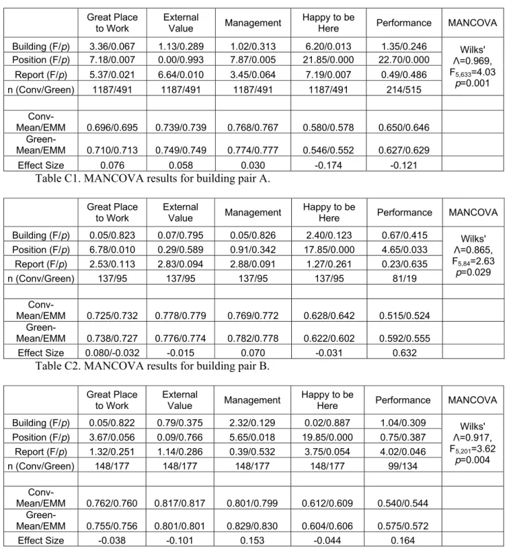
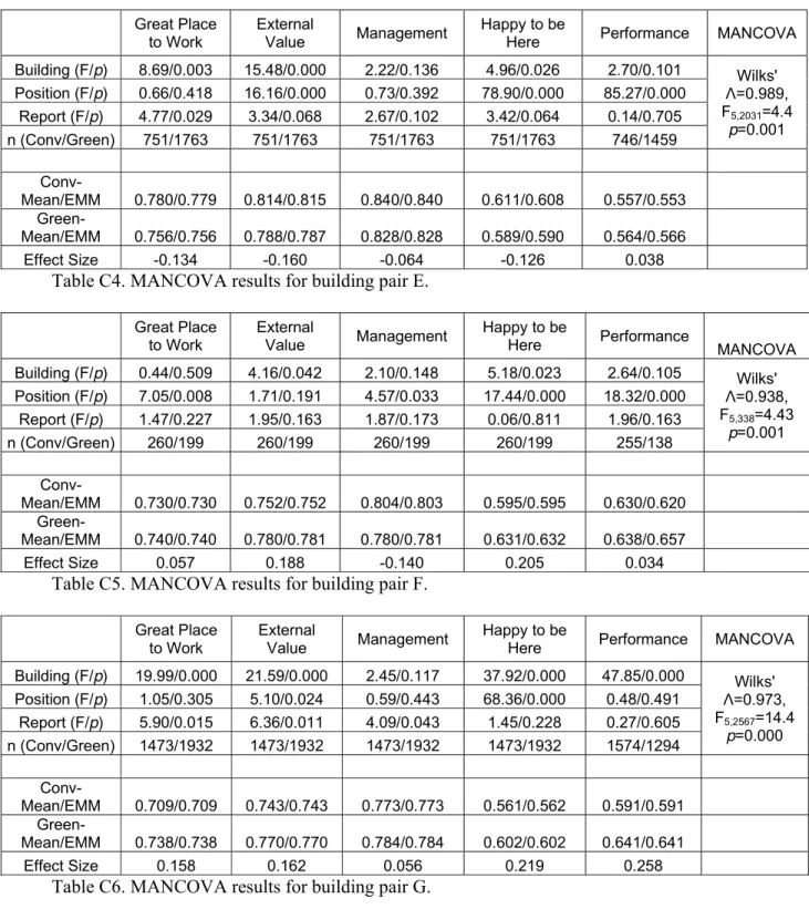
Table 8 summarizes the findings of the MANCOVAs on each building pair; the detailed statistical tables are provided in Appendix C. In interpreting these results the focus should not be on any single test, but on the overall pattern of results. In this context, the results are compelling and reinforce the trends in the building-level

findings. First, note that there were statistically significant overall MANCOVA tests for nine of the 10 building pairs.

Turning to the univariate ANCOVA tests for these pairs, a preponderance of effects favouring the green-certified building in the paired buildings was observed. For ‘Great Place to Work’, there were effects meeting the statistical criterion for five of the 10 building pairs, and in four of five cases the green-certified building was more highly rated than its conventional counterpart. For ‘External Value’, there were effects for five building pairs, and in four of these cases the green-certified building was more highly rated. For ‘Management’, there were only two pairs with differences in scores, but in both cases the green-certified building was more highly rated. For ‘Happy to be Here’, there were effects for five building pairs, and in three of these cases the green-certified building was more highly rated. For ‘Manager-assessed Performance’, there were only two pairs that met the criterion for statistically-significant differences in scores, but in both cases the green-certified building was more highly rated.

These effects are all in the small or small-medium range as defined by the Cohen’s d effect size statistic (see Appendix C for details). Nevertheless, small effects can have substantial practical impact, depending on the context. The study

organization’s HR group can judge the importance of the differences observed between building types in this analysis. A senior HR manager at the host organization had the following to say: “We are delighted to have partnered on this ground breaking study. The analysis shows how our sustainability policy and use of green buildings creates a positive environment that improves employee engagement … We look forward to uncovering new insights to assist in developing physical spaces …”

17 Pair ID  MANCOVA 

ANCOVA  EOS_Great  Place to  Work   EOS_External  Value  EOS_  Management  EOS_Happy  to be Here  Manager‐ assessed  Performance  A  _***  *  **  B  D  _**  E  _***  ***  ***  **  F  _{***  **  **}  G  _***  ***  ***  ***  ***  I  _{***  **  *  ***}  J  _***  ***  ***  **  ***  K  _**  L  _{*  **} 

Table 8. Summary of results of MANCOVA tests comparing matched green-conventional building pairs at the individual employee data level. Shaded cells with asterisks indicate a better outcome for the green-certified building in the pair; unshaded cells with asterisks indicate a better outcome for the conventional building in the pair; empty cells indicate no significant difference between buildings in the pair on that outcome. The detailed statistics are shown in the Appendix C.

Signif. Codes (p‐value): *** 0.01 ** 0.05 * 0.1. Bold cell outlines indicate that the effect size, expressed  as Cohen’s d, was > .20, or “small”.  

Conclusions

Many organizations, including the study organization, have pursued policies to add ‘green’ features to their office building portfolios to support key corporate sustainability goals, including improvements to the working environment for their employees. The results of this study support such policies. Overall, green-certified buildings

demonstrated higher values of corporate metrics related to organizational productivity compared to otherwise similar conventional buildings. Specifically, scores on the employee opinion survey (EOS), and manager-assessed job performance, were generally higher for green-certified buildings, with fewer instances of relatively poor scores.

These results support the hypothesis that being in a green (LEED-certified) building positively influences how occupants view their organization and conduct their work. This could be a direct effect (the employer is viewed positively because they have invested in a “better” building for the respondents), or an indirect effect (the green building has a superior indoor environment, which facilitates better comfort, mood and working conditions). Nevertheless, it is important to note that not all green buildings outperformed all conventional buildings, and superior performance was not exhibited on all outcomes examined.

Overall, these results are consistent with other studies demonstrating the benefits of green buildings on occupant satisfaction [e.g. Newsham et al, 2013] and extend the causal chain from better buildings to job satisfaction and other outcomes of more direct relevance to organizational productivity [Thompson et al, 2014; Alker (Ed.), 2014; MacNaughton et al, 2017].

18

Further, these results related to organizational productivity complement studies looking at other aspects of the financial benefits of green buildings. For example, several studies have analysed whether green buildings have higher real-estate value compared to otherwise similar conventional buildings [Devine & Kok, 2015]. In some cases green buildings are conflated with other sustainability categories or simply energy efficient buildings (e.g. Energy Star), but in general the results show that sustainable buildings tend to have lower vacancy rates, higher lease costs, and higher resale value.

Although these findings were derived from a richer dataset than has been referenced in the green buildings research literature to date, they should be considered preliminary. The number of individual occupants who contributed data was very large, but the number of buildings forming a valid comparison set was still relatively small. The matching of buildings on characteristics other than green certification was reasonable for a practical set of buildings, but was imperfect. Results were also based on a single year of data only. Therefore, although the trends favouring green-certified buildings were consistent, other explanations for differences cannot be completely ruled out. Nevertheless, these findings suggest that further analyses of this kind should be encouraged, and are likely to be fruitful in confirming and extending these findings. The strength of the conclusions will be greater if future investigations have larger datasets, and clearer differentiation between green and conventional buildings.

While the great potential of leveraging pre-existing organizational data for buildings-related research was clearly demonstrated, some uncertainties in derivation of these data did reduce the strength of the analyses. For example, the exact mapping of EOS items to scales was not known. This is understandable given that the original EOS stakeholders did not have this end use in mind. The recognition of the supplemental value of these datasets shown by this work may lead to greater attention to how data are prepared and documented, thus increasing the utility of organizational data.

Finally, these promising results are associated with whole-building differences (green-certified vs. conventional), which subsume much variation at the individual building system and indoor environment level. Further research to establish which specific green building features contribute to the observed benefits6, and which features dilute such effects, would be valuable to practitioners making design decisions.

Disclosure statement

No potential conflict of interest was reported by the authors.

Funding

This work was funded by the National Research Council of Canada’s High Performance Buildings Program. The study organization made an in-kind contribution of the data and its preparation.

Geolocation information

19

Acknowledgements

The authors are indebted to many people at the study organization who facilitated the development of this project and provided access to data and other valuable information, in particular: John Wylie, Ruth Weiner, Sorin Nitoi, Robert Carlyle and Jason Bernardon. Thanks are also due to several colleagues at NRC who played important roles in the delivery of this project: Dino Zuppa and Trevor Nightingale were key in developing the relationship between NRC and the study organization, and Alexandra Thompson provided suggestions on the approach to analysis, results interpretation, and report review.

References

Alker, J. E (Editor). 2014. Health, Wellbeing & Productivity in Offices: The next chapter for green building. World Green Building Council (WGBC). http://www.worldgbc.org/activities/health-wellbeing-productivity-offices/ Brill, M., Margulis, S. T., Konar, E., & BOSTI Associates (Eds.). 1984. Using office

design to increase productivity. Buffalo, NY: Workplace Design and Productivity.

Best, B. 2014. True or False: Saving Energy in the Workplace Automatically Drives Productivity.

http://www.energymanagertoday.com/true-false-saving-energy-workplace-automatically-drives-productivity-0105930/

Cohen, J. 1988. Statistical Power Analysis for the Behavioral Sciences (2nd ed.). Hillsdale, NJ: Erlbaum.

Devine, A.; Kok, N. 2015. Green certification and building performance: implications for tangibles and intangibles. The Journal of Portfolio Management, 41(6), pp. 151-163.

Frontczak, M.; Schiavon, S.; Goins, J.; Arens, E.; Zhang, H.; Wargocki, P. 2012. Quantitative relationships between occupant satisfaction and satisfaction aspects of indoor environmental quality and building design. Indoor Air, 22, pp. 119-131.

Gou, Z.; Lau, S.-Y.; Shen, J. 2011. Indoor environmental satisfaction in two LEED offices and its implications in green interior design. Indoor and Built Environment, 21(4), pp. 503–514.

Kaplan, R.S; Norton, D.P. 1992. The balanced scorecard - measures that drive performance. Harvard Business Review, Jan-Feb.

MacNaughton, P.; Satish, U.; Cedeno Laurent, J.G.; Flanigan, S.; Vallarino, J.; Coull, B. ; Spengler, J. D.; Allen, J. G. 2017. The impact of working in a green certified building on cognitive function and health. Building and Environment, 114, pp. 178–186.

Moschandreas, D. J.; Nuanual, R. M. 2008. Do certified sustainable buildings perform better than similar conventional buildings? International Journal of

Environment and Sustainable Development, 7(3), pp. 276-292.

Newsham, G.R., Birt, B.J., Arsenault, C., Thompson, A.J.L., Veitch, J.A., Mancini, S., Galasiu, A.D., Gover, B.N., Macdonald, I.A., Burns, G.J. 2013. Do Green Buildings Have Better Indoor Environments? New Evidence. Building Research & Information, 41(4), pp. 415-434.

Pritchard, R. D. 1992. Organizational productivity. In M. D. Dunnette & L. M. Hough (Eds.), Handbook of industrial and organizational psychology (2nd ed., Vol. 3, pp. 443-471). Palo Alto, CA: Consulting Psychologists Press.

20

Raudenbush, S.W.; Bryk, A.S. 2002. Hierarchical Linear Models. Applications and

Data Analysis Methods. Newbury Park, CA: Sage, 2nd ed.

Rosenthal, R. 1984. Parametric measures of effect size. In H. Cooper & L.V. Hedges (Eds.), The handbook of research synthesis, pp. 231-244. New York: Russell Sage Foundation.

Siegel, S.; Castellan, N. J. 1988. Nonparametric Statistics for the Behavioral Sciences (2nd edition). New York: McGraw-Hill.

Sundstrom, E. 1986. Work places: The psychology of the physical environment in offices and factories. New York: Cambridge University Press.

Thatcher, A.; Milner, K. 2012. The impact of 'green' building on employees' physical and psychological wellbeing. Work, 41, pp. 3816-3823.

Thompson, A.J.L.; Veitch, J.A.; Newsham, G.R. 2014. Improving Organizational Productivity with Building Automation Systems. Continental Automated Buildings Association (CABA), Ottawa, Canada.

https://www.caba.org/CABA/DocumentLibrary/Public/ImprovingProductivityB AS.aspx

21

Appendix A: Characteristics of the large office buildings not used in the analyses

Building Characteristics Characteristics of Employees in each Building

B u ildi n g ID Green Pending Re g io n Total Are a Occ upie d b y Stu d y Organ iz ation R a ng e (f t 2 ) Nu m b e r o f Emplo y ee s Ma p ped to Build in g Ra nge Dens ity C o ns tr u c ti on Da te Gende r Ag e Degre e Commute (k m) Depen d e n t

Total Pay (lo

c al $) Po si ti o n Re p o rt FTPT Tenur e ( y rs ) Actio n X2 0 Western US <50,001 101-500 3.53 1971-1980 0.78 38.1 3.7 14.0 2.4 202,500 5.4 0.2 1.00 4.6 0.8 X4 1 Southern Ontario <50,001 101-500 6.83 1981-1990 0.47 45.1 3.2 34.3 2.2 97,913 5.7 3.6 1.00 8.4 1.0 X6 0 Eastern US 50,001-100,000 101-500 2.39 After 2000 0.36 43.6 3.0 30.7 2.5 85,111 5.3 3.6 0.99 6.5 1.2 X7 0 Northeast US <50,001 101-500 2.73 1981-1990 0.64 48.4 3.4 25.2 2.8 113,000 5.1 1.8 1.00 7.7 0.5 X10 0 Western Canada <50,001 <101 3.27 1991-2000 0.42 42.3 3.1 14.3 2.3 55,487 3.7 3.2 0.81 8.9 1.3 X11 0 Western Canada <50,001 <101 3.56 1971-1980 0.46 44.5 2.9 19.9 2.4 59,013 3.9 1.1 0.82 10.4 1.4 X14 0 Western Canada <50,001 101-500 2.85 1971-1980 0.35 43.9 2.9 14.8 1.9 56,273 3.7 0.9 0.86 9.3 1.1

X15 1 Southern Ontario >500,000 1,001-5,000 5.27 After 2000 0.50 43.7 3.1 33.9 2.4 93,625 5.5 9.4 0.99 8.6 1.0

X16 0 Southern Ontario >500,000 1,001-5,000 5.50 After 2000 0.52 41.7 3.1 33.6 2.4 77,789 4.9 5.8 0.99 7.3 0.9

X19 0 Southern Ontario >500,000 >5,000 7.17 After 2000 0.38 40.7 2.8 22.9 2.5 50,369 3.6 5.7 0.96 7.7 1.5

X20 1 Southern Ontario 200,001-500,000 1,001-5,000 7.83 1971-1980 0.37 44.0 2.8 32.3 2.3 51,328 3.9 5.7 0.98 8.9 0.9 X24 0 Southern Ontario 100,001-200,000 1,001-5,000 7.01 1981-1990 0.36 43.4 2.7 22.1 2.4 43,878 2.9 2.1 0.92 9.2 1.5 X25 0 Western Canada 50,001-100,000 101-500 8.99 1971-1980 0.36 41.2 2.6 16.0 2.1 41,801 2.5 2.0 0.89 7.9 1.8 X27 0 Southern Ontario <50,001 101-500 3.83 1971-1980 0.42 44.5 2.8 18.6 2.3 60,000 4.0 3.0 0.92 9.3 0.9 X30 0 Southern Ontario <50,001 101-500 3.19 1981-1990 0.44 42.3 3.0 19.1 2.8 66,134 4.2 1.0 0.93 8.2 0.9 X31 0 Western Canada <50,001 101-500 3.92 1971-1980 0.39 45.6 2.4 7.4 2.2 55,470 3.6 2.4 0.85 9.6 0.9 X33 0 Quebec 50,001-100,000 501-1,000 8.65 1971-1980 0.43 38.0 2.7 16.6 2.2 39,584 2.7 3.1 0.89 7.8 2.4 X34 0 Southern Ontario <50,001 101-500 3.16 1971-1980 0.35 46.2 3.1 22.5 2.3 73,891 4.5 14.0 0.94 9.7 1.1

X36 1 Eastern Canada <50,001 101-500 3.48 After 2000 0.45 44.9 3.2 14.0 2.1 81,162 4.7 15.3 0.94 10.1 0.7

22 X42 0 Southern Ontario <50,001 101-500 3.18 1991-2000 0.47 43.4 2.8 28.3 2.8 67,152 4.4 4.2 0.94 8.8 0.8 X43 0 Western Canada 50,001-100,000 501-1,000 14.98 1991-2000 0.41 38.5 2.7 10.0 2.3 39,343 2.6 2.0 0.91 6.7 2.5 X44 0 Quebec <50,001 101-500 3.57 1981-1990 0.37 41.5 3.0 22.3 2.2 59,493 4.2 4.5 0.89 9.2 1.5 X47 0 Quebec 100,001-200,000 1,001-5,000 9.49 0.54 35.2 2.9 15.2 2.0 44,614 2.9 2.5 0.94 6.2 2.2 X48 0 Central US 200,001-500,000 1,001-5,000 4.14 1991-2000 0.53 41.9 3.2 23.6 2.5 76,250 4.3 6.0 0.98 7.9 0.9 X50 0 Eastern Canada 50,001-100,000 501-1,000 14.62 1991-2000 0.38 38.9 2.4 14.3 2.1 41,296 2.6 2.4 0.94 7.6 2.6

Table A1. Characteristics of the large office buildings not used in the analyses. Density=mapped employees/1000 ft2;

Gender=”"mean” gender (female=0, male=1) of employees in the building; Age=mean age of occupants; Degree=mean level of education reached (e.g. 3= Bachelor’s Degree); Commute=median commuting distance; Dependent=mean number of dependents in occupants’ families; Total Pay=median annual compensation; Position=mean position in hierarchy (higher value indicates higher position); Report=mean number of direct and indirect reports; FTPT=mean ratio of full-time to part-time employees (0=all part-time, 1=all full-time); Tenure=mean time employed at study organization; Action=mean number of staffing actions per employee.

23

Appendix B: Scores for each outcome for large office buildings not used in the analyses

Building Info EOS_ Great Place to Work EOS_ External Value EOS_ Management EOS_ Happy to be Here Manager-assessed Performance Building ID Gre e n Pendi n g

mean sd mean sd mean sd mean sd EOS_n mean sd n

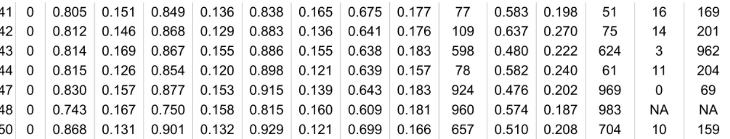
HVAC Co m p lai n ts To tal Co m p lai n ts X2 0 0.618 0.202 0.687 0.191 0.702 0.214 0.551 0.184 66 0.700 0.112 5 NA NA X4 1 0.677 0.214 0.713 0.200 0.735 0.231 0.550 0.196 240 0.544 0.185 259 13 323 X6 0 0.702 0.202 0.749 0.163 0.755 0.222 0.546 0.217 105 0.601 0.154 104 NA NA X7 0 0.706 0.199 0.760 0.176 0.759 0.206 0.579 0.212 90 0.656 0.146 40 NA NA X10 0 0.726 0.176 0.779 0.148 0.777 0.202 0.591 0.179 88 0.574 0.207 64 6 316 X11 0 0.730 0.169 0.773 0.161 0.794 0.178 0.621 0.150 78 0.582 0.201 67 0 268 X14 0 0.744 0.174 0.792 0.163 0.818 0.158 0.613 0.207 83 0.587 0.227 72 1 170 X15 1 0.746 0.178 0.773 0.162 0.800 0.197 0.590 0.182 2999 0.594 0.169 3076 4 494 X16 0 0.707 0.192 0.751 0.170 0.767 0.201 0.554 0.188 3703 0.603 0.180 3114 497 7534 X19 0 0.757 0.185 0.810 0.165 0.829 0.187 0.582 0.187 4583 0.531 0.192 4588 244 6006 X20 1 0.749 0.181 0.793 0.163 0.803 0.200 0.578 0.172 1276 0.573 0.165 1288 102 962 X24 0 0.761 0.188 0.823 0.168 0.827 0.192 0.560 0.182 1090 0.554 0.173 746 252 1351 X25 0 0.761 0.199 0.810 0.175 0.843 0.191 0.585 0.192 385 0.497 0.184 428 2 277 X27 0 0.768 0.182 0.827 0.160 0.820 0.204 0.641 0.161 119 0.595 0.237 95 1 27 X30 0 0.777 0.151 0.831 0.137 0.809 0.179 0.619 0.166 82 0.528 0.164 62 1 95 X31 0 0.778 0.175 0.824 0.149 0.839 0.180 0.637 0.175 117 0.542 0.223 90 8 187 X33 0 0.782 0.175 0.825 0.166 0.876 0.159 0.601 0.180 513 0.539 0.167 317 82 423 X34 0 0.785 0.167 0.813 0.158 0.862 0.159 0.633 0.185 122 0.596 0.216 104 2 133 X36 1 0.788 0.169 0.813 0.152 0.823 0.197 0.661 0.164 114 0.583 0.218 102 5 75

24 X41 0 0.805 0.151 0.849 0.136 0.838 0.165 0.675 0.177 77 0.583 0.198 51 16 169 X42 0 0.812 0.146 0.868 0.129 0.883 0.136 0.641 0.176 109 0.637 0.270 75 14 201 X43 0 0.814 0.169 0.867 0.155 0.886 0.155 0.638 0.183 598 0.480 0.222 624 3 962 X44 0 0.815 0.126 0.854 0.120 0.898 0.121 0.639 0.157 78 0.582 0.240 61 11 204 X47 0 0.830 0.157 0.877 0.153 0.915 0.139 0.643 0.183 924 0.476 0.202 969 0 69 X48 0 0.743 0.167 0.750 0.158 0.815 0.160 0.609 0.181 960 0.574 0.187 983 NA NA X50 0 0.868 0.131 0.901 0.132 0.929 0.121 0.699 0.166 657 0.510 0.208 704 10 159

Table B1. Mean and standard deviation of scores for each outcome for each large office buildings not used in the analyses, and total complaint counts. EOS_n=number of respondents to EOS survey; HVAC

Complaints=total number of complaints used in analysed HVAC complaints outcome; Total complaints= total number of complaints from all sources; NA=not available.

25

Appendix C: Details of MANCOVA Analysis

The effect size calculated in these analyses is Cohen’s d, which is the difference in means divided by the standard deviation (s.d.). The difference in means uses the raw means, shown in the tables below. For the s.d. a “pooled” s.d. from the s.d.’s of each building for an outcome variable was calculated, which is complicated by different sample sizes in each building. The formula is below, where nx=number of data points from building x, and sx=s.d. of outcome data in building x.

To interpret effect sizes, Cohen [1988] described an effect size of 0.2 as ‘small’ and gives as an example that the difference between the heights of 15 year old and 16 year old girls in the US corresponds to an effect of this size. An effect size of 0.5 is described as ‘medium’ and is ‘large enough to be visible to the naked eye’. A 0.5 effect size corresponds to the difference between the heights of 14 year old and 18 year old girls. Cohen describes an effect size of 0.8 as ‘grossly perceptible and therefore large’ and equates it to the difference between the heights of 13 year old and 18 year old girls. As a further example he states that the difference in IQ between holders of the Ph.D. degree and ‘typical college freshmen’ is comparable to an effect size of 0.8.

[http://www.leeds.ac.uk/educol/documents/00002182.doc]

Key to tables below:

Effect Size values >0.2 are shown in bold. n = number of respondents in each building

EMM = estimated marginal means, the means predicted by the model, thus representing the mean values in each building type after taking co-variates into account.

Of the 65 separate ANCOVA tests six show a difference in raw means in the opposite direction to the difference in estimated marginal means (EMM). In five of these cases the EMM difference favours the green buildings, reflected in the test in the ‘Buildings’ row of the tables. In these six cases the effect size was also estimated based on the EMMs and the standard deviation of the predicted values in the model. In all six cases the effect sizes were very small, and there was no implication for the interpretation of the pattern of test results overall.

26 Great Place to Work External Value Management Happy to be

Here Performance MANCOVA

Building (F/p) 3.36/0.067 1.13/0.289 1.02/0.313 6.20/0.013 1.35/0.246 _Wilks' Λ=0.969, F5,633=4.03 p=0.001 Position (F/p) 7.18/0.007 0.00/0.993 7.87/0.005 21.85/0.000 22.70/0.000 Report (F/p) 5.37/0.021 6.64/0.010 3.45/0.064 7.19/0.007 0.49/0.486 n (Conv/Green) 1187/491 1187/491 1187/491 1187/491 214/515 Conv-Mean/EMM 0.696/0.695 0.739/0.739 0.768/0.767 0.580/0.578 0.650/0.646 Green-Mean/EMM 0.710/0.713 0.749/0.749 0.774/0.777 0.546/0.552 0.627/0.629 Effect Size 0.076 0.058 0.030 -0.174 -0.121

Table C1. MANCOVA results for building pair A.

Great Place

to Work

External

Value Management

Happy to be

Here Performance MANCOVA

Building (F/p) 0.05/0.823 0.07/0.795 0.05/0.826 2.40/0.123 0.67/0.415 Wilks' Λ=0.865, F5,84=2.63 p=0.029 Position (F/p) 6.78/0.010 0.29/0.589 0.91/0.342 17.85/0.000 4.65/0.033 Report (F/p) 2.53/0.113 2.83/0.094 2.88/0.091 1.27/0.261 0.23/0.635 n (Conv/Green) 137/95 137/95 137/95 137/95 81/19 Conv-Mean/EMM 0.725/0.732 0.778/0.779 0.769/0.772 0.628/0.642 0.515/0.524 Green-Mean/EMM 0.738/0.727 0.776/0.774 0.782/0.778 0.622/0.602 0.592/0.555 Effect Size 0.080/-0.032 -0.015 0.070 -0.031 0.632

Table C2. MANCOVA results for building pair B.

Great Place

to Work

External

Value Management

Happy to be

Here Performance MANCOVA

Building (F/p) 0.05/0.822 0.79/0.375 2.32/0.129 0.02/0.887 1.04/0.309 Wilks' Λ=0.917, F5,201=3.62 p=0.004 Position (F/p) 3.67/0.056 0.09/0.766 5.65/0.018 19.85/0.000 0.75/0.387 Report (F/p) 1.32/0.251 1.14/0.286 0.39/0.532 3.75/0.054 4.02/0.046 n (Conv/Green) 148/177 148/177 148/177 148/177 99/134 Conv-Mean/EMM 0.762/0.760 0.817/0.817 0.801/0.799 0.612/0.609 0.540/0.544 Green-Mean/EMM 0.755/0.756 0.801/0.801 0.829/0.830 0.604/0.606 0.575/0.572 Effect Size -0.038 -0.101 0.153 -0.044 0.164

27 Great Place to Work External Value Management Happy to be

Here Performance MANCOVA

Building (F/p) 8.69/0.003 15.48/0.000 2.22/0.136 4.96/0.026 2.70/0.101 _Wilks' Λ=0.989, F5,2031=4.4 p=0.001 Position (F/p) 0.66/0.418 16.16/0.000 0.73/0.392 78.90/0.000 85.27/0.000 Report (F/p) 4.77/0.029 3.34/0.068 2.67/0.102 3.42/0.064 0.14/0.705 n (Conv/Green) 751/1763 751/1763 751/1763 751/1763 746/1459 Conv-Mean/EMM 0.780/0.779 0.814/0.815 0.840/0.840 0.611/0.608 0.557/0.553 Green-Mean/EMM 0.756/0.756 0.788/0.787 0.828/0.828 0.589/0.590 0.564/0.566 Effect Size -0.134 -0.160 -0.064 -0.126 0.038

Table C4. MANCOVA results for building pair E.

Great Place

to Work

External

Value Management

Happy to be

Here Performance _MANCOVA

Building (F/p) 0.44/0.509 4.16/0.042 2.10/0.148 5.18/0.023 2.64/0.105 _Wilks' Λ=0.938, F5,338=4.43 p=0.001 Position (F/p) 7.05/0.008 1.71/0.191 4.57/0.033 17.44/0.000 18.32/0.000 Report (F/p) 1.47/0.227 1.95/0.163 1.87/0.173 0.06/0.811 1.96/0.163 n (Conv/Green) 260/199 260/199 260/199 260/199 255/138 Conv-Mean/EMM 0.730/0.730 0.752/0.752 0.804/0.803 0.595/0.595 0.630/0.620 Green-Mean/EMM 0.740/0.740 0.780/0.781 0.780/0.781 0.631/0.632 0.638/0.657 Effect Size 0.057 0.188 -0.140 0.205 0.034

Table C5. MANCOVA results for building pair F.

Great Place

to Work

External

Value Management

Happy to be

Here Performance MANCOVA

Building (F/p) 19.99/0.000 21.59/0.000 2.45/0.117 37.92/0.000 47.85/0.000 Wilks' Λ=0.973, F5,2567=14.4 p=0.000 Position (F/p) 1.05/0.305 5.10/0.024 0.59/0.443 68.36/0.000 0.48/0.491 Report (F/p) 5.90/0.015 6.36/0.011 4.09/0.043 1.45/0.228 0.27/0.605 n (Conv/Green) 1473/1932 1473/1932 1473/1932 1473/1932 1574/1294 Conv-Mean/EMM 0.709/0.709 0.743/0.743 0.773/0.773 0.561/0.562 0.591/0.591 Green-Mean/EMM 0.738/0.738 0.770/0.770 0.784/0.784 0.602/0.602 0.641/0.641 Effect Size 0.158 0.162 0.056 0.219 0.258

28 Great Place to Work External Value Management Happy to be

Here Performance MANCOVA

Building (F/p) 5.67/0.018 3.22/0.074 14.69/0.000 0.50/0.480 0.01/0.940 _Wilks' Λ=0.884, F5,163=4.29 p=0.001 Position (F/p) 8.25/0.004 0.23/0.633 3.42/0.066 10.25/0.002 1.81/0.181 Report (F/p) 0.55/0.459 0.94/0.334 0.18/0.669 0.38/0.541 0.17/0.684 n (Conv/Green) 88/139 88/139 88/139 88/139 73/112 Conv-Mean/EMM 0.730/0.736 0.798/0.799 0.779/0.783 0.613/0.620 0.565/0.575 Green-Mean/EMM 0.793/0.789 0.835/0.834 0.873/0.870 0.642/0.637 0.585/0.578 Effect Size 0.381 0.264 0.563 0.159 0.082

Table C7. MANCOVA results for building pair I.

Great Place

to Work

External

Value Management

Happy to be

Here Performance MANCOVA

Building (F/p) 31.64/0.000 25.32/0.000 5.61/0.018 6.84/0.009 1.31/0.252 _Wilks' Λ=0.891, F5,506=12.35 p=0.000 Position (F/p) 1.44/0.231 2.59/0.108 1.47/0.226 32.00/0.000 0.07/0.785 Report (F/p) 0.03/0.861 0.01/0.914 0.29/0.592 1.66/0.198 4.94/0.027 n (Conv/Green) 218/423 218/423 218/423 218/423 178/385 Conv-Mean/EMM 0.689/0.691 0.747/0.744 0.799/0.801 0.568/0.581 0.574/0.574 Green-Mean/EMM 0.781/0.779 0.813/0.815 0.840/0.839 0.626/0.619 0.596/0.596 Effect Size 0.506 0.398 0.226 0.327 0.103

Table C8. MANCOVA results for building pair J.

Great Place

to Work

External

Value Management

Happy to be

Here Performance MANCOVA

Building (F/p) 0.03/0.861 1.90/0.168 0.29/0.591 0.16/0.688 0.46/0.497 _Wilks' Λ=0.975, F5,389=1.96 p=0.083 Position (F/p) 13.01/0.000 0.04/0.847 9.82/0.002 27.78/0.000 6.53/0.011 Report (F/p) 1.05/0.306 0.46/0.500 0.54/0.463 0.68/0.411 0.01/0.906 n (Conv/Green) 99/390 99/390 99/390 99/390 84/353 Conv-Mean/EMM 0.747/0.744 0.805/0.805 0.827/0.824 0.620/0.616 0.580/0.581 Green-Mean/EMM 0.747/0.748 0.780/0.780 0.812/0.813 0.607/0.608 0.564/0.564 Effect Size -0.001/0.020 -0.157 -0.078 -0.073 -0.080

29 Great Place to Work External Value Management Happy to be

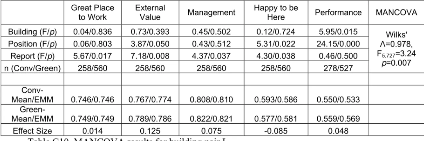
Here Performance MANCOVA

Building (F/p) 0.04/0.836 0.73/0.393 0.45/0.502 0.12/0.724 5.95/0.015 _Wilks' Λ=0.978, F5,727=3.24 p=0.007 Position (F/p) 0.06/0.803 3.87/0.050 0.43/0.512 5.31/0.022 24.15/0.000 Report (F/p) 5.67/0.017 7.18/0.008 4.37/0.037 4.30/0.038 0.46/0.500 n (Conv/Green) 258/560 258/560 258/560 258/560 278/527 Conv-Mean/EMM 0.746/0.746 0.767/0.774 0.808/0.810 0.593/0.586 0.550/0.533 Green-Mean/EMM 0.749/0.749 0.789/0.786 0.822/0.821 0.577/0.581 0.559/0.569 Effect Size 0.014 0.125 0.075 -0.085 0.048

30 ENDNOTES

1

The colloquial phrase “green building” is shorthand to describe buildings with certified sustainable features. In the context of this project this means LEED-certified buildings. 2

One way to estimate the order of magnitude of the frequency of a change in building location, given the data available, was to look at the frequency of changes in reporting centre postal code, which in most, but not all cases would be associated with a change in an employee’s ‘home’ building. The five quarterly data loads from Jan. 2014 – Jan. 2015 were examined, in which there were complete postal codes for 18,993 employees in the 23 buildings later considered for inclusion in the green-conventional building pairs (and of which 20 were chosen for the final analysis). Of these 17,665 (93%) demonstrated no change in reporting centre postal code over the one year period.

3

The number of complaints in other categories was generally very low, except for reporting of burn-out lamps, which was not judged to be linked to green-certification.

4

Differences in the characteristics of the buildings (other than green certification) are still controlled for implicitly via the matching process.

5

Another approach to analysis with data at the individual level is hierarchical linear modelling (HLM), in which individuals (Level 1) are nested in buildings (Level 2), which are nested in green-conventional pairs/groups (Level 3). Conceptually, this method involves regressing the outcome variable of interest on predictors at Level 1 (e.g. EOS outcome) and then the regression coefficients becoming the outcome variables for a regression at Level 2, and so on. Predictor variables may then be applied at each level; i.e. properties of individuals at Level 1 (e.g. age, gender), properties of buildings at Level 2 (e.g. size, age), and properties of pairs/groups at Level 3 (e.g. location/climate). This method has become particularly popular in research on student educational outcomes, where students (Level 1) may be nested within classrooms with different properties, including, possibly, teacher characteristics (Level 2), nested within schools with different properties (Level 3) [Raudenbush & Bryk, 2002]. A challenge with this method is that it is ‘data hungry’ requiring simplification choices to be made in model specification, and the results can often be difficult to interpret. This method was applied to the data with results that were consistent with the results of the other methods used, exhibiting the same trends. However, other methods are highlighted in this report due to their relative conceptual simplicity and ease of interpretation.

6

And what features cause some conventional buildings to score highly on some HR-related metrics.