Université de Montréal
Liquides ioniques électroactifs dans la composition
d’électrolytes avancés pour des applications en énergie
Electroactive ionic liquids in advanced electrolyte composition for energy application
Par Bruno Gélinas
Département de chimie Faculté des Arts et des Sciences
Thèse présentée à laFaculté des études supérieures et postdoctorales en vue de l’obtention du grade dephilosophiae doctor(Ph.D.) en chimie
Avril 2017 © Bruno Gélinas 2017
i
Résumé
Cette thèse contribue au développement de nouveaux électrolytes pour améliorer la sécurité des batteries à ion lithium par le biais d’une étude et du développement d'électrolytes avancés à base de nouveaux liquides ioniques. En utilisant des approches synthétiques nouvellement développées, plusieurs liquides ioniques électroactifs, qui sont obtenus en modifiant le cation ou l'anion du liquide ionique, sont étudiés pour comprendre comment la structure des constituants ioniques du sel affecte ses propriétés physico-chimiques et électrochimiques. La méthodologie générale qui a guidé le travail tout au long de la thèse doit établir des comparaisons entre des liquides ioniques similaires qui présentent le groupe redox sur le cation et sur l'anion. Les progrès réalisés dans la compréhension des liquides ioniques redox dans cette thèse ont permis leur application dans plusieurs types de dispositifs de stockage d'énergie. La thèse décrira comment les électrolytes avancés basés sur ces liquides ioniques ont été appliqués pour éviter la surcharge des électrodes positives dans les batteries à ion lithium, pour améliorer la sécurité en réduisant l'inflammabilité, pour augmenter la concentration des additifs utilisant leur grande solubilité, pour augmenter la densité énergétique des supercapaciteurs et afin d'obtenir des espèces électrochromes stables avec l'air et avec l'humidité dans les dispositifs électrochromiques autoblanchiments. Cette thèse contribue au domaine du stockage d'énergie en améliorant les électrolytes et au domaine du liquide ionique en fournissant de nouvelles méthodes de synthèse, de nouvelles structures ioniques et une meilleure compréhension du fondamental des liquides ioniques électroactifs.
Mots-clés : Électrochimie, piles à ion lithium, synthèse de liquides ioniques, espèce électroactive, électrolyte concentré et navette redox.
ii
Abstract
This thesis contribute to the development of new electrolytes to improve the safety of lithium-ion batteries through the study and development of advanced electrolytes based on novel ionic liquids. Using newly developed synthetic approaches, several electroactive ionic liquids, which are obtained by modifying either the cation or the anion of the ionic liquid, are studied to understand how the structure of the salt’s ionic constituents affect its physico-chemical and electrochemical properties. The general methodology that guided the work throughout the whole thesis has to establish comparisons between similar ionic liquids that present the redox group on the cation and on the anion. The progress that has been made in understanding redox ionic liquids in this thesis allowed their application in several types of energy storage devices. The thesis will describe how advanced electrolytes based on these ionic liquids have been applied to prevent overcharging positive electrode materials in lithium-ion batteries, to improve safety by decreasing flammability, to increase the concentration of additives over their solubility, to increase energy density of supercapacitors and to achieve air- and moisture-stable electrochromic species for self-bleaching electrochromic devices. This thesis contributes to the field of energy storage by improving electrolytes and to the domain of ionic liquid by providing new synthesis methods, novel ion structures, and a better understanding of the fundamental of electroactive ionic liquids. Keywords: Electrochemistry, lithium ion batteries, synthesis of ionic liquids, electroactive species, concentrated electrolyte and redox shuttle.
iii
Table des matières
Résumé ... i
Abstract ... ii
Liste des tableaux ... xi
Liste des figures ... xvi
Liste des abréviations et symboles ... xxxvi
Remerciements ... xl Chapitre 1 : Introduction aux électrolytes avancés ... 1
1.1. Avant-propos ... 1
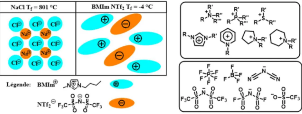
1.2. Introduction aux liquides ioniques et aux liquides ioniques fonctionnels ... 1
1.2.1. Mise en contexte des liquides ioniques et généralité ... 1
1.2.2. Les liquides ioniques fonctionnels ... 4
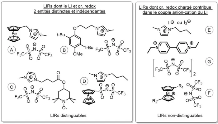
1.2.3. Les liquides ioniques électroactifs et leurs applications ... 5
1.3. Mise en contexte des batteries à ion lithium et les surtensions ... 7
1.3.1. Les batteries à ion lithium ... 7
1.3.2. Problématique des piles à ion lithium ... 9
1.3.3. Mécanismes de protection des surtensions de l’électrode positive ... 12
1.3.4. Navette redox pour la protection des surtensions ... 15
1.4. Électrolytes utilisés dans les batteries à ion lithium ... 19
1.4.1. Les électrolytes utilisés pour les batteries à ion lithium ... 19
1.4.2. Fenêtre électrochimique des électrolytes et les matériaux d’électrode positive ... 21
1.4.3. Les liquides ioniques sans solvant comme électrolyte dans les batteries à ion lithium ………... 22
1.4.4. Les électrolytes concentrés et les liquides ioniques solvatés comme électrolyte . 23 1.4.5. Mélange de carbonates et de liquides ioniques comme électrolyte ... 25
iv
1.5. Les supercaciteurs et leur électrolytes électroactifs ... 26
1.5.1. Comparaison entre les supercapaciteurs et les batteries à ion lithium. ... 26
1.5.2. Électrolyte des supercapaciteurs et électrolyte électroactive. ... 28
1.6. Description de la thèse et objectifs ... 30
1.7. Références ... 31
Chapitre 2 : Théorie et techniques expérimentales ... 40
2.1. Avant-propos et mise en contexte ... 40
2.2. Synthèse de liquides ioniques avancés ... 40
2.2.1. Synthèse des liquides ioniques fonctionnalisés. ... 40
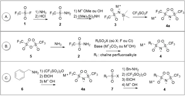
2.2.2. Synthèse de l’anion bis(trifluorométhylsulfonyl)imide. ... 41
2.2.3. Synthèse de chlorure de sulfonyle. ... 43
2.3. Analyses physicochimiques ... 44
2.3.1. Analyses thermiques ... 44
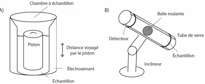
2.3.2. Viscosité dynamique ... 47
2.3.3. Présence d’eau par titrage coulométrique de Karl-Fisher ... 48
2.3.4. L’autodiffusion par résonance magnétique nucléaire ... 50
2.4. Analyses électrochimiques ... 57
2.4.1. Spectroscopie d’impédance et conductivité ionique ... 57
2.4.2. Méthodes voltampérométriques et ampérométriques ... 59
2.4.3. Analyse de charge/décharge galvanostatique en pile bouton ... 74
2.5. Références ... 85
Chapitre 3 : L’effet des chaînes latérales d’un imidazolium à base de ferrocényle ... 87
3.1. Avant-propos et mise en contexte ... 87
3.2. Article: Conductivity and Electrochemistry of Ferrocenyl-Imidazolium Redox Ionic Liquids with Different Alkyl Chain Lengths... 88
3.2.1. Abstract ... 88
v
3.2.3. Experimental ... 90
3.2.4. Results and Discussion ... 92
3.2.5. Conclusions ... 102 3.2.6. Acknowledgments... 103 3.2.7. References ... 103 3.3. Supplementary Material ... 104 3.3.1. Synthesis ... 104 3.3.2. References ... 106
Chapitre 4: Synthèse et caractérisation d’un liquide ionique utilisant un anion électroactif ... 107
4.1. Avant-propos et mise en contexte ... 107
4.2. Article: Synthesis and characterization of an electroactive ionic liquid based on the ferrocenylsulfonyl(trifluoromethylsulfonyl)imide anion ... 108
4.2.1. Highlights ... 108
4.2.2. Abstract ... 108
4.2.3. Introduction ... 110
4.2.4. Experimental ... 111
4.2.5. Results and discussion ... 116
4.2.6. Conclusions ... 128
4.2.7. Acknowledgments... 128
4.2.8. Appendix A. Supplementary data ... 128
4.2.9. References ... 129 4.3. Supporting Information ... 132 4.3.1. Synthesis ... 132 4.3.2. NMR analysis... 133 4.3.3. Thermal analysis ... 138 4.3.4. Electrochemical analysis ... 139
Chapitre 5 : Propriétés de transport et électrochimiques d’un liquide ionique électroactif et de l’ion de lithium ... 144
vi
5.1. Avant-propos et mise en contexte ... 144
5.2. Article: Electrochemical and transport properties of ions in mixtures of electroactive ionic liquid and propylene carbonate with a lithium salt for lithium-ion batteries... 145
5.2.1. Abstract ... 145
5.2.2. Introduction ... 146
5.2.3. Experimental Section ... 149
5.2.4. Results and Discussion ... 151
5.2.5. Conclusions ... 168
5.2.6. Associated Content ... 168
5.2.7. Acknowledgments... 169
5.2.8. References ... 169
5.3. Suppporting Information ... 173
5.3.1. Synthetic procedure of Lithium Ferrocenylsulfonyl (trifluoromethylsulfonyl)imide (Li [FcNTf]) in two step procedure. ... 174
5.3.2. Summary of self-diffusion analysis ... 175
5.3.3. Viscosity measurements... 176
5.3.4. Electrochemical analysis and additional figures ... 177
5.3.5. LiTi2(PO4)3 preparation and X-Ray diffraction ... 179
Chapitre 6 : Liquide ionique électroactif utilisant un anion redox basé sur le ferrocène pour contrer les surtensions ... 181
6.1. Avant-propos et mise en contexte ... 181
6.2. Bifunctional ionic liquids to improve Lithium-ion battery electrolytes ... 182
6.2.1. Abstract ... 182
6.2.2. Introduction ... 183
6.2.3. Experimental ... 186
6.2.4. Results and discussion ... 189
6.2.5. Conclusions ... 208
6.2.6. Acknowledgments... 208
vii
6.3. Supporting Information ... 213
6.3.1. Synthetic procedure of redox shuttle ... 214
6.3.2. Thermal analysis ... 217
6.3.3. Extra CVs and electrochemical analysis ... 221
6.3.4. Complete viscosity/ionic conductivity study and flammability test ... 224
6.3.5. Extra Galvanostatic charge-overcharge-discharge curves and rate capability study 229 6.3.6. References ... 230
Chapitre 7 : Liquide ionique électroactif basé sur la modification du centre redox diméthoxybenzène comme navette redox ... 231
7.1. Avant-propos et mise en contexte ... 231
6.3. Electroactive ionic liquids based on 2,5-ditert-butyl-1,4-dimethoxybenzene and triflimide anion as redox shuttle for LFP/LTO lithium-ion batteries ... 232
7.2.1. Abstract ... 232
7.2.2. Introduction ... 233
7.2.3. Experimental ... 235
7.2.4. Results and discussion ... 239
7.2.5. Conclusions ... 259
7.2.6. Acknowledgments... 259
7.2.7. References ... 259
7.3. Supporting Information ... 263
7.3.1. General procedure for the preparation of dimethoxybenzene (3,4) and 1,4-bis(2,2,2-trifluoroethoxy)benzene (5,6) ... 264
7.3.2. Preparation of (2,5-ditert-butyl-4-methoxyphenoxy)propylsulfonyl chloride (8) 264 7.3.3. General procedure for the preparation of 2,5-dimethoxyphenylsulfonyl chloride and 1,4-bis(2,2,2-trifluoroethoxy)phenylsulfonyl chloride (12, 13 and 21) ... 265
7.3.4. General procedure for the preparation of sodium electroactive triflimide salt (11-13, 18 and 22) ... 265
viii
7.3.5. General procedure for the preparation of electroactive triflimide ionic liquids
(14-16, 19 and 23) ... 265
7.3.6. Synthesis characterization such as MS, NMR and elemental analysis ... 266
7.3.7. NMR spectra ... 271
7.3.8. Thermal analysis ... 296
7.3.9. Extra CVs of DDB and DDBF... 298
7.3.10. Arrhenius/Eyring plots of ionic conductivity/fluidity... 299
7.3.11. Reference ... 301
Chapitre 8 : Dispositif électrochromique utilisant un anion redox à base de ferrocène et le viologène... 302
8.1. Avant-propos et mise en contexte ... 302
8.2. Air-stable, self-bleaching electrochromic device based on viologen and ferrocene-containing triflimide redox ionic liquids... 303
8.2.1. Table of contents graphic: ... 303
8.2.2. Abstract ... 303
8.2.3. Introduction ... 304
8.2.4. Experimental ... 307
8.2.5. Results and discussion ... 311
8.2.6. Conclusions ... 328
8.2.7. Acknowledgments... 329
8.2.8. References ... 329
8.3. Supporting information ... 333
8.3.1. Synthesis of FcNTf redox ionic liquids and viologen ... 334
8.3.2. XPS analysis of BMIm Fc(II)NTf and Fc(III)NTf ... 337
8.3.3. Thermal analysis ... 343
8.3.4. Extra cyclic voltammetry and chronoamperometry ... 345
8.3.5. References ... 349
Chapitre 9 : Conclusions et perspectives ... 350
ix
9.2. Résumé et conclusions générales ... 350
9.3. Travaux futurs ... 353
Annexe 1: L’effet de la chaîne latérale d’un liquide ionique utilisant un anion électroactif ... 355
A1.1. Avant-propos et mise en contexte ... 355
A1.2. Article: Electrochemical and physicochemical properties of redox ionic liquids using electroactive anions: influence of alkylimidazolium chain length ... 356
A1.2.1. Highlights ... 356
A1.2.2. Abstract ... 356
A1.2.3. Introduction ... 357
A1.2.4. Experimental ... 359
A1.2.4. Results and discussion ... 361
A1.2.5. Conclusions ... 370
A1.2.6. Acknowledgments ... 371
A1.2.7. Appendix A. Supplementary data ... 371
A1.2.8. References ... 371
A1.3. Supporting Information ... 374
A1.3.1. Synthesis of redox ionic liquids and imidazolium cation ... 375
A1.3.2. Thermal analysis ... 380
A1.3.3. Electrochemical analysis ... 381
A1.3.4. UV-Vis spectrum ... 383
Annexe 2 : Liquide ionique électroactif pour les supercapaciteurs ... 384
A2.1. Avant-propos et mise en contexte ... 384
A2.2. Article: Redox-active electrolyte supercapacitors using electroactive ionic liquids .... 385
A2.2.1. Highlights ... 385
A2.2.2. Abstract ... 386
A2.2.3. Introduction ... 387
x
A2.2.5. Results and Discussion... 388
A2.2.6. Conclusions ... 394
A2.2.7. Acknowledgments ... 394
xi
Liste des tableaux
Chapitre 1
Tableau 1.1. Avantages et désavantages des différentes méthodes pour contrôler les surcharges. ... 13 Tableau 1.2. Potentiel d’équilibre de quelques N-Rs utilisées pour la protection des BILs ... 16 Tableau 1.3. Différentes conductivités ioniques selon l’électrolyte avec l’application
correspondante à 25 °C. ... 19 Tableau 1.4. Électrolytes non-aqueux classiques pour la BILs ... 20
Chapitre 3
Table 3.1. Ionic conductivities and molar ionic conductivities of the pure RILs and VFT fitting parameters. ... 94 Table 3.2. Ionic conductivities and viscosities of RIL solutions in EC/DEC 1:2 (v/v) at 25°C . 96 Table 3.3. Self-diffusion coefficient of FcEImC4-TFSI at different concentrations in EC:DEC
(1:2) solvent. ... 98 Table 3.4. Equilibrium potentials for FcEImCn-TFSI and the oxidation limit of the RIL in solution.
Data was obtained from CV recorded at 100 mV ·s−1 and all potentials are given vs. the Fc+/Fc couple (+0.55 V vs. NHE). ... 101 Table 3.5. Diffusion coefficients for oxidation of RIL (FcEImC1, FcEImC4, FcEImC8 and
FcEImC12) ... 101
CHAPITRE 4
Table 4.1. Physicochemical properties of neat BMIm NTf2 and BMIm FcNTf ... 117 Table 4.2. Electrochemical parameters using CV, RDE voltammetry and DPSC of 1 mM Fc or
xii
Table 4.3. Potential parameters obtained from cyclic voltammograms of 10 mM and 1.4 M solutions of BMIm FcNTf in CH3CN with 1.0 M TBAP at 100 mV s-1. The potentials are given vs. the Fc/Fc+ couple. ... 127
Table S4.1. Data obtained from CV analysis for the calculation of rate constants for the oxidation of Fc or BMIM FcNTf (2 mM) in CH3CN with 0.1 M TBAP as supporting electrolyte. ... 141 Table S4.2. Rate constants for the oxidation of Fc or BMIM FcNTf in CH3CN with 0.1 M TBAP
as supporting electrolyte. ... 142
Chapitre 5
Table 5.1. Midpoint Potentials and Diffusion Coefficients for Reduction Form of 0.3 mol dm– 3 [BMIm][FcNTf] in Various Concentrations of [BMIm][NTf
2] and Li[NTf2] as Supporting Electrolytea ... 153 Table 5.2. All electrolyte parameters using CV, NMR and AC impedance (Electrolyte 1: 1.0 mol
dm-3 of Li [NTf
2] in PC; Electrolyte 2: 0.3 mol dm-3 of [BMIm] [FcNTf] and 1.0 mol dm-3 of Li [NTf2] in PC; Electrolyte 3: 0.3 mol dm-3 of Li [FcNTf] and 0.7 mol dm-3 of Li [NTf2] in PC). ... 165 Table 5.3. The electrochemical characterisation of Li/LTP cell at 0.1 C rate for the 5th cycle in
different electrolytes (Electrolyte A: 1.0 mol dm-3 of Li [NTf
2] in EC-DEC 1:2 v/v; Electrolyte B: 0.3 mol dm-3 of [BMIm] [FcNTf] and 1.0 mol dm-3 of Li [NTf
2] in EC-DEC 1:2 v/v; Electrolyte C: 0.3 mol dm-3 of Li [FcNTf] and 1.0 mol dm-3 of Li [NTf
2] in EC-DEC 1:2 v/v). ... 167
Chapitre 6
Table 6.1. Potential parameters obtained from cyclic voltammograms at 100 mV s-1 of 10 mM [FcEMIm][NTf2], [BMIm][FcNTf] and Li[FcNTf] in EC-DEC 1:2 (v/v) with 1.0 M Li[NTf2]. ... 192 Table 6.2. Transport properties using CV and DPSC of 10 mM [FcEMIm][NTf2],
xiii
Table 6.3. The viscosity, ionic conductivity, activation energies, entropy and enthalpy for fluidity and ionic conductivity of redox-active electrolytes (EC-DEC 1:2 (v/v) with 1.0 M Li[NTf2]). ... 201 Table 6.4. Electrochemical characterisation of Li/LTP cells in different redox-active electrolytes.
(IL: [BMIm][NTf2]) ... 205
Table S6.1. Thermochemical properties of neat [FcEMIm][NTf2] and [BMIm][FcNTf]. ... 217 Table S6.2. Advanced electrolytes using EC-DEC 1:2 (v/v) as solvents were characterized in the
complete study. ... 224 Table S6.3. All viscosities (η), activation energies of fluidity (φ = 1/η) (Ea,φ), entropy (ΔS φ) and
enthalpy (ΔH φ) of [FcNTf] solutions in EC-DEC 1:2 (v/v) with or without Li [NTf2] are summarized. ... 225 Table S6.4. All ionic conductivities (σ), activation energies of ionic conductivity (Ea,σ), entropy
(ΔSσ) and enthalpy (ΔHσ) of [FcNTf] solution in EC-DEC 1:2 (v/v) with or without Li [NTf2] are summarized. ... 226
Chapitre 7
Table 7.1. Thermochemical properties of neat organic RILs based on DDB and triflimide anion. ... 241 Table 7.2. Potential parameters obtained from cyclic voltammograms at 100 mV s-1 of 10 mM
DDB, DDBF, [BMIm] [DDB-pNTf], [BMIm] [MDB-NTf] and [BMIm] [MDBF-NTf] in EC-DEC 1:2 (v/v) with 1.0 M Li [NTf2]. ... 247 Table 7.3. Transport properties using CV and DPSC of 10 mM DDB, DDBF, [BMIm] [DDB-pNTf] and [BMIm] [MDB-NTf] in EC-DEC 1:2 (v/v) with 1.0 M Li [NTf2]. ... 250 Table 7.4. All viscosities (η), activation energies of fluidity (φ = 1/η) (Ea,φ), entropy (ΔSφ) and
enthalpy (ΔHφ) of 0.3 M RIL electrolyte in EC-DEC 1:2 (v/v) with 1.0 M Li [NTf2]. ... 252 Table 7.5. All ionic conductivities (σ), activation energies of ionic conductivity (Ea,σ), entropy
(ΔSσ) and enthalpy (ΔHσ) of 0.3 M RIL electrolyte in EC-DEC 1:2 (v/v) with 1.0 M Li [NTf2]. ... 252
xiv Chapitre 8
Table 8.1. Thermochemical properties of neat [FcNTf] and [EV] RIL. ... 312
Table 8.2. Potential parameters obtained from CV at 100 mV s-1 of 10 mM solution of [EV] dication and [FcNTf] anion in [BMIm] [NTf2]. ... 314
Table 8.3. Transport properties using DPSC of 10 mM RIL such as [BMIm] [FcNTf], [BPyr] [FcNTf], [Me3BuN] [FcNTf], [MBPip] [FcNTf] and [Fc(III)NTf] in corresponding common IL ([Fc(III)NTf] and [EV] [NTf2]2 in [BMIm] [NTf2]). Diffusion coefficients were calculated from Shoup and Szabo fit. ... 317
Table 8.4. Performance of [FcNTf]/[EV]/IL ECD with an applied asymmetric square wave between 0 and 2.0 V during 30 s for each potential step where the bleaching and coloring times are defined as the time required to reach 95% ΔT at 610 nm ... 328
Table S8.1. Conditions of XPS experiment. ... 337
Table S8.2. Identification and quantification of elements following the survey. ... 337
Table S8.3. Identification of chemical bonds following the high-resolution spectrum. ... 338
Annexe 1 Table A1.1. Physicochemical properties of [CxCyIm][FcNTf] and its corresponding common IL. The values in italic are from other sources (see footnote). ... 362
Table A1.2. VFT fitting parameters of [CxCxIm][FcNTf] in their undiluted state. The parameters for the RILs with C8 chains are not listed because of unreliable fitting. ... 365
Table A1.3. Diffusion coefficients of 0.3 M and 1 mM [CxCxIm][FcNTf] in acetonitrile with 1M TBAP. ... 367
xv
Table A1.4. Electrochemical parameters for 0.3 M and 1 mM [CxCxIM][FcNTf] in acetonitrile with 1 M TBAP at a scan rate of 100 mV s-1. Oxidation and reduction limit at 0.3 M... 367
Annexe 2
Table A2.1. Specific energy values (during discharge) at different maximum voltages and iR drop obtained for the devices (charge and discharge currents of 2 mA). ... 391
xvi
Liste des figures
Chapitre 1
Figure 1.1. Définition des liquides ioniques et quelques exemples d’anions et de cations. ... 3 Figure 1.2. Exemples de liquides ioniques fonctionnels (LIFs) utilisant plusieurs groupements
fonctionnels (GF). ... 5 Figure 1.3. Exemples de liquides ioniques électroactifs qui sont classés comme suit : LIRs
distinguables et non-distinguables. ... 6 Figure 1.4. Principe de la batterie à ion lithium. ... 8 Figure 1.5. Densité d’énergie gravimétrique et volumétrique des différentes technologies des
batteries. (Tirée de Armand & Tarascon (2001). Nature, Ref. 35) ... 9 Figure 1.6. Schématisation d’une batterie complètement déchargée (A) et partiellement chargée
(B) avec un module avec une faible capacité qui est complètement chargée. (Adaptée de Chen, Z., Y. Qin, et al. (2009). Electrochim. Acta, Ref. 37) ... 10 Figure 1.7. Corrélation entre le potentiel et la température d’une cellule à ion lithium prismatique
avec une surcharge à une vitesse de charge de 1 C. (Tirée de Satoh et al., (2005), J. Power Sources, Ref. 40) ... 11 Figure 1.8. Réactions exothermiques de la décomposition du LiCoO2 comme matériel d’électrode
positive (À gauche) et le diagramme à bande correspondant qui représente l’appauvrissement en électron à l’électrode positive lors d’une surcharge. (À droite) ... 12 Figure 1.9. Mécanisme de la navette redox (N-R, Redox Shuttle). ... 14 Figure 1.10. Aperçu de quelques navettes redox (N-Rs) de la littérature pour les BILs. ... 15 Figure 1.11. Voltage selon la capacité pour différents matériaux d’électrode relatifs à une fenêtre
électrochimique (Eg de l’électrolyte montré sur la figure) utilisant un électrolyte de 1 mol dm -3 de Li PF
6 dans EC-DEC (1:1 v/v). (Tirée de Goodenough et al., (2010), Chem. Mater., Ref. 80) ... 22 Figure 1.12. Schéma qui différencie les électrolytes concentrés et les liquides ioniques solvatés
où Kcomplex est la contante d’équilibre pour le complexe et (Tirée de Watanabe et al., (2010), PCCP, Ref. 100) ... 23
xvii
Figure 1.13. Profile de charge-décharge en fonction de différentes densités de courant pour une cellule de Li/LiCoO2 utilisant l’électrolyte a) le perchlorate de lithium (1 mol dm-3) dans le carbonate de propylène et le Li(G4)1 NTf2 (2,75 mol dm-3 de lithium). (Tirée de Watanabe et al., (2012), J. Electrochem. Soc., Ref. 104) ... 25 Figure 1.14. Diagramme de Ragone représentant la densité d’énergie spécifique et la puissance
spécifique des batteries, dont la BIL et des supercapaciteurs électrochimiques. (Tirée de Banks (2011). RSC Adv., Ref. 125) ... 27
Chapitre 2
Figure 2.1. Schéma illustrant la différence entre la fonctionnalisation d’un anion ou d’un cation reposant sur le couple imidazolium et bis(sulfonyl)imide. ... 41 Figure 2.2. Schéma illustrant la synthèse d’anion basé sur le bis(perfluoroalkyl)sulfonyl) imide ... 42 Figure 2.3. Schéma illustranst la synthèse de chlorure de sulfonyle. ... 44 Figure 2.4. A) L’analyse thermogravimétrique (ATG) et l’analyse calorimétrique différentielle
(ACD) B) à compensation de puissance et C) à flux de chaleur. ... 46 Figure 2.5. A) viscosimètre à piston oscillant et B) viscosimètre à bille. ... 48 Figure 2.6. Cellule du coulomètre Karl Fisher... 50 Figure 2.7. A) Processus de relaxation T1 et T2 B) Séquence à gradient pulsé. La séquence est
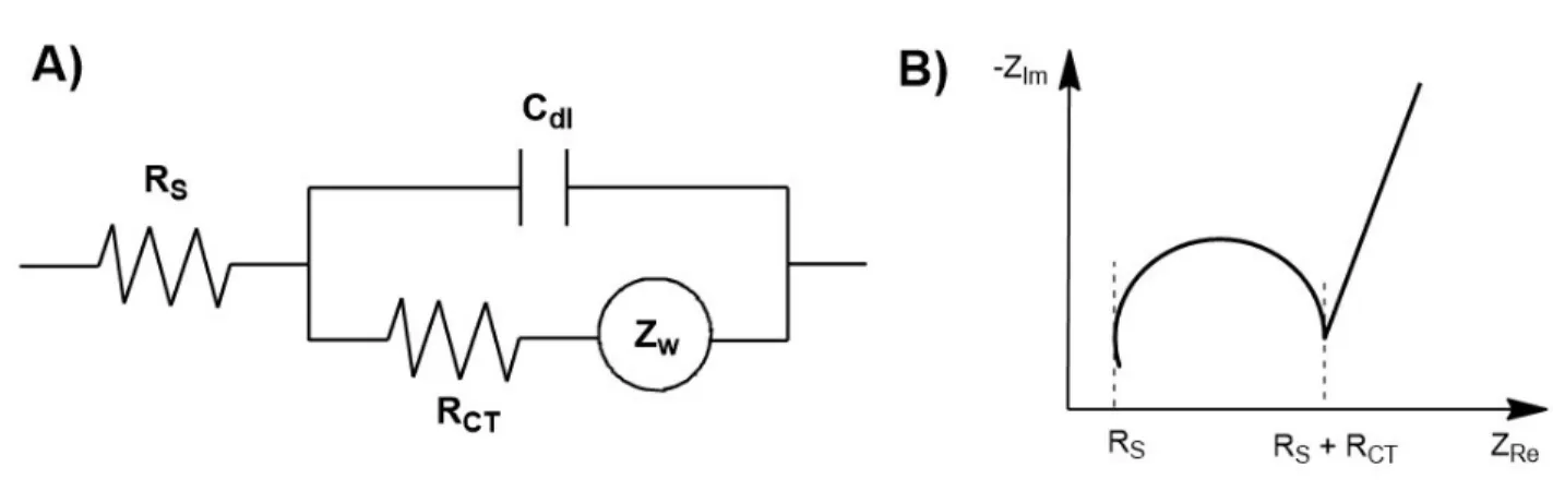
appliquée pour un système C) sans diffusion/sans gradient, D) sans diffusion/avec gradient et E) avec diffusion/avec gradient. ... 52 Figure 2.8. Séquences spin-écho versus spin-écho stimulé. ... 55 Figure 2.9. A) Circuit équivalent de Randle et B) diagramme de Nyquist typique. ... 57 Figure 2.10. Route typique pour une espèce électroactive lors d’une réaction électrochimique.
Illustration reproduite de la Ref.[26]. ... 60 Figure 2.11. Illustration de l’oxydation et de la réduction des espèces électroactives. ... 62 Figure 2.12. A) Rampe de balayage linéaire pour la voltampérométrie cyclique et B) un
voltampérogramme cyclique typique pour une espèce électroactive réversible. ... 64 Figure 2.13. A) Montage expérimental d’une cellule à trois électrodes en voltampérométrie
xviii
Figure 2.14. A) Rampe de balayage linéaire pour la voltampérométrie à électrode rotative et B) un voltampérogramme à électrode rotative typique pour une espèce électroactive réversible. ... 68 Figure 2.15. A) Programmation d’une expérience de chronoampérométrie lors d’une oxydation
suivie d’une réduction utilisant préalablement un temps d’équilibre. Le potentiel appliqué est constant. B) Courbe ampérométrique pour une espèce électroactive réversible et diffusionnelle. ... 70 Figure 2.16. Illustration du transport de masse A) pour une macroélectrode via une diffusion
planaire, B) pour une macroélectrode via une convection et C) pour une microélectrode via une diffusion radiale. ... 70 Figure 2.17. A) Rampe de balayage impulsionnelle pour la voltammétrie impulsionnelle à vagues
carrées et B) un voltampérogramme impulsionnel à vagues carrées typique pour une espèce électroactive réversible. L’exemple présente une réaction d’oxydation. ... 73 Figure 2.18. A) composition d’une électrode composite et B) Composante d’une pile bouton. . 75 Figure 2.19. Polarisation de cellule pour la décharge. ... 77 Figure 2.20. Illustration qui montre la différence entre l’énergie et la puissance. ... 81 Figure 2.21. Des courbes galvanostatiques montrant A) une courbe charge-décharge sans navette
redox et B) une courbe charge-surcharge-décharge utilisant une navette redox présent dans l’électrolyte. ... 84
Chapitre 3
Figure 3.1. Structure of redox ionic liquids (RILs) used given with their corresponding abbreviation (n=0: FcEImC1; n=3: FcEImC4; n=7: FcEImC8; n=11: FcEImC12) ... 90 Figure 3.2. Synthetic steps of the ferrocenyl-imidazolium redox ionic liquids (RILs). ... 91 Figure 3.3. a) Temperature dependence on the ionic conductivity of pure redox ionic liquids b)
Arrhenius plots for the FcEImC4 in EC/DEC 1:2 with or without of LiTFSI. Measurements were done at 5 °C intervals between 25 and 75 °C. ... 95 Figure 3.4. Cyclic voltammograms (scan rate of 100 mV s−1) for a) a 10% solution of RILs in
EC/DEC 1:2 with 1.5 M LiTFSI and b) different concentrations of FcEImC4 (1, 10 and 50%) in EC/DEC 1:2 with and without 1.5 M LiTFSI. c) CVs of 10% FcEImC4 in EC/DEC 1:2
xix
(v/v) with 1.5 M LiTFSI at scan rates ranging from 25–500 mV s−1; d) Randles Sevcik Plot of Ip vs v1/2. ... 100
Chapitre 4
Figure 4.1. Chemical structure of 1-butyl-3-methylimidazolium ferrocenylsulfonyl (trifluoromethylsulfonyl)imide (BMIm FcNTf) and 1-butyl-3-methylimidazolium bis(trifluoromethylsulfonyl)imide (BMIm NTf2). ... 111 Figure 4.2. Synthetic pathway of BMIm FcNTf. ... 113 Figure 4.3. A) Temperature dependence on the ionic conductivity of neat BMIm NTf2 (■) and
BMIm FcNTf (●). Measurements were done at an interval of 4 °C from 80 to 32 °C. B) Arrhenius plot for the viscosity of neat BMIm NTf2 (■) and BMIm FcNTf (●). Measurements were done at an interval of 4 °C from 80 to 56 °C. Data of BMIm NTf2 from Watanabe and co-workers.[42] ... 118 Figure 4.4. Walden plot with an increase of temperature of neat BMIm NTf2 (■) and BMIm FcNTf
(●). Measurements were done at an interval of 4 °C from 80 to 56 °C. Data of BMIm NTf2 from Watanabe and co-workers.[42] ... 119 Figure 4.5. A) CVs of 1 mM BMIm FcNTf in CH3CN with 0.1 M TBAP at various scan rates. B)
Randles-Sevcik plot of 1 mM Fc (■) and BMIm FcNTf (●) in CH3CN with 0.1 M TBAP. The scan rates used were 25 to 1000 mV s-1. ... 121 Figure 4.6. A) RDE voltammetry at 100 mV s-1 of 1 mM BMIm FcNTf in CH
3CN with 0.1 M TBAP at various rotating rates. B) Levich plot of 1 mM Fc (■) and BMIm FcNTf (●) in CH3CN with 0.1 M TBAP. The rotating rates used were 100 to 2500 RPM. ... 121 Figure 4.7. DPSC using a microelectrode of 1 mM of Fc (■) and BMIm FcNTf (●) in CH3CN
with 0.1 M TBAP. The duration τ was used 5 s. The initial and final potentials were -0.38 V [Fc] and -0.18 V [FcNTf]. The step potentials were 0.42 V [Fc] and 0.62 V [FcNTf]. (Potential vs. Fc/Fc+) Stojek plot for the oxidation (B) and reduction (C). ... 122 Figure 4.8. Nicholson plot of 2 mM of Fc (■) and BMIm FcNTf (●) in CH3CN with 0.1 M TBAP.
The scan rates used were 35 to 75 V s-1. ... 123 Figure 4.9. CVs (A) at 50 mV s-1 and SWV (B) using P
w: 10 ms, PH: 50 mV and SH: 1 mV. Electroactive species were 10 mM of Fc and 10 mM of BMIm FcNTf in CH3CN and
xx
supporting electrolytes were 0.75M of BMIm NTF2 (Black line) or Li NTf2 (Red line). C) Difference of equilibrium potential between Fc and FcNTf dependence on supporting electrolyte concentration. (■: CV using BMIm NTf2; ●: CV using Li NTf2; ♦: SWV using BMIm NTf2; ▲: SWV using Li NTf2) ... 125 Figure 4.10. A) CVs of 50% (v/v) of BMIm FcNTf in CH3CN with 1.0 M TBAP (Black line) and
50% (v/v) BMIm FcNTf in CH3CN without supporting electrolyte (Red line). Scan rate used was 100 mV s-1. B) Representation of the film formed on the electrode following the oxidation of the FcNTf anion at high concentrations and in the absence of supporting electrolyte. Solvent (CH3CN) was omitted for clarity. ... 127
Figure S4.1. 1H NMR (DMSO-d 6, 300 MHz): δ (ppm) = 4.99 (s, 2H, Cp-SO2Cl), 4.81 (s, 2H, Cp-SO2Cl), 4.46 (s, 5H, Cp). (FcSO2Cl) ... 133 Figure S4.2. 1H NMR (DMSO-d 6, 300 MHz): δ (ppm) = 4.53 (s, 2H, Cp-SO2Cl), 4.28 (s, 7H, Cp-SO2Cl + Cp). (Na FcNTf) ... 133 Figure S4.3. 19F NMR (DMSO-d 6, 282 MHz): δ (ppm) = -77.62(-CF3). (Na FcNTf) ... 134 Figure S4.4. 13C NMR (DMSO-d 6, 125 MHz): δ (ppm) = 121.90(-CF3); 119.32(-CF3); 94.61(Cp-SO2Cl); 70.44(Cp); 69.19(Cp); 68.61(Cp). (Na FcNTf) ... 134 Figure S4.5. 1H NMR (DMSO-d 6, 300 MHz): δ (ppm) = 9.10 (s,1H,Im+), 7.73 (d,2H,Im+), 4.54 (t,2H,Cp-SO2Cl), 4.29 (s,7H, Cp-SO2Cl+Cp), 4.16 (t,2H,-CH2Im+), 3.85 (s,3H, CH3Im+), 1.76 (m,2H,-CH2-) 1.26 (m,2H,-CH2-), 0.90 (t,3H,-CH3). (BMIm FcNTf) ... 135 Figure S4.6. 19F NMR (DMSO-d 6, 282 MHz): δ (ppm) = -77.63(-CF3). (BMIm FcNTf) ... 135 Figure S4.7. 13C NMR (DMSO-d
6, 125 MHz): δ (ppm) = 136.97(Im+); 124.09(Im+); 122.74(Im+); 121.89(-CF3); 119.32(-CF3); 94.58(Cp-SO2Cl); 70.44(Cp); 60.21(Cp); 68.60(Cp); 48.99(CH3Im+); 36.25(-CH2Im+); 31.82(-CH2-); 19.23(-CH2-); 13.71(-CH3). (BMIm FcNTf) ... 136 Figure S4.8. 1H NMR (DMSO-d 6, 300 MHz): δ (ppm) = 9.24 (s,1H,Im+), 7.77 (d,2H,Im+), 4.17 (t,2H,-CH2Im+), 3.86 (s,3H, CH3Im+), 1.76 (m,2H,-CH2-) 1.25 (m,2H,-CH2-), 0.89 (t,3H,-CH3). (BMIm Br) ... 136 Figure S4.9. 13C NMR (DMSO-d
6, 125 MHz): δ (ppm) = 136.99(Im+); 124.05(Im+); 122.72(Im+); 48.91(CH3Im+); 36.23(-CH2Im+); 31.82(-CH2-); 19.22(-CH2-); 13.74(-CH3). (BMIm Br) 137 Figure S4.10. TGA of neat BMIm FcNTf with a ramp of 10°C per minute. ... 138
xxi
Figure S4.11. Modulated DSC of neat BMIm FcNTf. The measurements were done between -50 to 65°C during 2 cycles with a ramp of 1 °C per minute and with isothermal of 5 minutes between the cooling and heating. The parameter of modulation was ±0.11°C every 40 seconds. First cycle (black line) and second cycle (red line). ... 138 Figure S4.12. A) CVs of 1 mM of Fc in CH3CN with 0.1 M TBAP at various scan rates. The scan
rates used were 25 to 1000 mV s-1. B) RDE voltammetry at 100 mV s-1 of 1 mM of Fc in CH3CN with 0.1 M TBAP at various rotating rates. The rotating rates used were 100 to 2500 RPM. ... 139 Figure S4.13. A) CVs using a microelectrode of (0.5, 1.0 and 2.0) mM of Fc in CH3CN with 0.1
M TBAP at 10 mV s-1. ... 139 Figure S4.14. DPSC using a microelectrode of 1 mM of Fc (■) and BMIm FcNTf (●) in CH3CN
with 0.1 M TBAP. The duration τ was used 5 s. The initial potentials were 0.38 V [Fc] and -0.18 V [FcNTf]. The step potentials were 0.42 V [Fc] and 0.62 V [FcNTf] (Potential vs. Fc/Fc+). The Compton’s methodology and Shoup and Szabo fitting were used. ... 140 Figure S4.15. CV of 10 mM of BMIm FcNTf in CH3CN with 1.0 M TBAP at 100 mV s-1 shows
electrochemical potential window. ... 140 Figure S4.16. CVs (A) at 50 mV s-1 and SWV (B) using P
w: 10 ms, PH: 50 mV and SH: 1 mV. Electroactive species were 10 mM of Fc and 10 mM of BMIm FcNTf in CH3CN with various concentrations of BMIm NTf2. Reference electrode: Ag/AgNO3(sat.) in 0.1 M TBAP with CH3CN. ... 142 Figure S4.17. CVs (A) at 50 mV s-1 and SWV (B) using Pw: 10 ms, PH: 50 mV and SH: 1 mV.
Electroactive species were 10 mM of Fc and 10 mM of BMIm FcNTf in CH3CN with 1.0 M of IL of different anions such as BMIm NTf2 (black line), BMIm BF4 (red line) and BMIm PF6 (blue line). Reference electrode: Ag/AgNO3(sat.) in 0.1 M TBAP with CH3CN. ... 143 Figure S4.18. Difference of mid-point potential between Fc and BMIm FcNTf using CVs (A) and
SWV (B) in CH3CN with different electrolyte concentrations. ... 143
Chapitre 5
Figure 5.1. Chemical structure of 1-butyl-3-methylimidazolium bis(trifluoromethylsulfonyl)imide ([BMIm] [NTf2]), 1-butyl-3-methylimidazolium
xxii
ferrocenylsulfonyl(trifluoromethylsulfonyl)imide ([BMIm] [FcNTf]) and lithium ferrocenylsulfonyl(trifluoromethylsulfonyl)imide (Li [FcNTf]). ... 148 Figure 5.2. A) CVs of 0.3 mol dm-3 of [BMIm] [FcNTf] with 1.0 mol dm-3 Li [NTf
2] using various concentrations of [BMIm] [NTf2]. B) CVs of 0.3 M of [BMIm] [FcNTf] in pure PC with various concentrations of Li [NTf2]. All CVs was recorded at 100 mV s-1. ... 152 Figure 5.3. Diffusion coefficients from CV analysis as a function of various concentrations of
[BMIm] [NTf2] in PC with 0.3 mol dm-3 of [BMIm] [FcNTf] and 1.0 mol dm-3 of Li [NTf2] (orange) and various concentrations of Li [NTf2] in pure PC with 0.3 mol dm-3 [BMIm] [FcNTf] (blue). ... 155 Figure 5.4. Self-diffusion coefficients as a function of A) molar fraction of [BMIm] [FcNTf] in
neat [BMIm] [NTf2], B) various concentrations of [BMIm] [NTf2] in PC with 0.3 mol dm-3 of [BMIm] [FcNTf] and 1.0 mol dm-3 of Li [NTf
2] and C) various concentrations of Li [NTf2] in pure PC with 0.3 mol dm-3 [BMIm] [FcNTf]. ... 158 Figure 5.5. Apparent transference number of Li+, [NTf
2]-, [BMIm]+ and [FcNTf]- for A) various concentrations of [BMIm] [NTf2] with 0.3 mol dm-3 of [BMIm] [FcNTf] and 1.0 mol dm-3 of Li [NTf2] and B) various concentrations of Li [NTf2] in pure PC with 0.3 mol dm-3 [BMIm] [FcNTf]. NMR total ionic conductivities and apparent fractional ionic conductivities of Li+, [NTf2]-, [BMIm]+ and [FcNTf]- for C) various concentrations of [BMIm] [NTf2] with 0.3 mol dm-3 of [BMIm] [FcNTf] and 1.0 mol dm-3 of Li [NTf
2] and D) various concentrations of Li [NTf2] in pure PC with 0.3 mol dm-3 [BMIm] [FcNTf]. ... 160 Figure 5.6. NMR and AC ionic conductivities using various concentrations of [BMIm] [NTf2]
with 0.3 mol dm-3of [BMIm] [FcNTf] and 1.0 mol dm-3 of Li [NTf
2]. Ionicity is given by σAC/σNMR. Ionic conductivities were measured at room temperature. ... 163 Figure 5.7. A) Capacity profile of Li/LTP cell at 0.1 C rate and 10 h. overcharge for the 5th cycle
containing different electrolytes (Electrolyte A (Red line): 1.0 mol dm-3 of Li [NTf
2] in EC-DEC 1:2 v/v; Electrolyte B (Blue line): 0.3 mol dm-3 of [BMIm] [FcNTf] and 1.0 mol dm-3 of Li [NTf2] in EC-DEC 1:2 v/v; Electrolyte C (Orange line): 0.3 mol dm-3 of Li [FcNTf] and 1.0 mol dm-3 of Li [NTf
2] in EC-DEC 1:2 v/v). B) Capacity profile for the 5th (Blue line) and 50th (Red line) cycle containing Electrolyte C. ... 167
xxiii
Figure S5.1. Synthetic pathway of Lithium Ferrocenylsulfonyl (trifluoromethylsulfonyl)imide (Li [FcNTf])... 174 Figure S5.2. Stejskal-Tanner plots (Ln(I/I0) vs g2) of 0.3 M of [BMIm] [FcNTf] with 1.0 M LiNTf2 in pure PC using A) 1H, B) 19F and C) 7Li NMR. ... 175 Figure S5.3. Dynamic viscosity as a function of molar fraction of [BMIm] [FcNTf] in Neat IL ... 176 Figure S5.4. A) Randles-Sevcik plots (Ip vs v1/2) of 0.3 M of [BMIm] [FcNTf] with 1.0 mol dm-3 Li [NTf2] in PC using various concentrations of [BMIm] [NTf2]. B) Randles-Sevcik plots (Ip vs v1/2) of 0.3 mol dm-3 of [BMIm] [FcNTf] in pure PC with various concentrations of Li [NTf2]. The scan rates used were 50 to 1000 mV s-1. ... 177 Figure S5.5. CVs and Randles-Sevcik plots (Ip vs v1/2) 0.3 mol dm-3of Li [FcNTf] with 0.7 mol
dm-3 of Li [NTf
2] in PC. The scan rates used were 25 to 1000 mV s-1. ... 178 Figure S5.6. CVs of 0.3 mol dm-3of [BMIm] [FcNTf] with 1.0 mol dm-3 of Li [NTf
2] in PC (Electrolyte 2; black line) and 0.3 mol dm-3of Li [FcNTf] with 0.7 mol dm-3 of Li [NTf
2] in PC (Electrolyte 3; red line) at 100 mV s-1. ... 178 Figure S5.7. X-Ray diffraction (XRD) of LiTi2(PO4)3 (LTP), with R-3c space group indexation.
The star (*) refers to the Al sample holder. ... 180
Chapitre 6
Figure 6.1. Chemical structure of 1-(ferrocenylmethyl)-3-methylmidazolilium bis(trifluoromethylsulfonyl)imide ([FcEMIm][NTf2]) and 1-butyl-3-methylimidazolium ferrocenylsulfonyl (trifluoromethylsulfonyl)imide ([BMIm][FcNTf]) and lithium ferrocenylsulfonyl (trifluoromethylsulfonyl)imide (Li[FcNTf]). ... 185 Figure 6.2. Schematic illustration of the redox shuttle mechanism. ... 186 Figure 6.3. A) CVs of electroactive species of 10 mM solution of [FcEMIm][NTf2] (red line),
[BMIm][FcNTf] (orange line) and Li[FcNTf] (blue line) in EC-DEC 1:2 (v/v) with 1 M Li[NTf2] at 100 mV s-1. B) Randles-Sevcik plots of these electroactive solutions. The scan rates used were 10 to 750 mV s-1. ... 193
xxiv
Figure 6.4. CVs of comparison between different [FcNTf] solutions (0.3, 0.7 and 1.0 M) in EC-DEC 1:2 (v/v) with 1.0 M Li[NTf2] in presence or absence of [BMIm][NTf2] at A) 10 mV s-1 and B) 100 mV s-1. ... 195 Figure 6.5. A) DPSC using a microelectrode of 10 mM [FcEMIm][NTf2] (red line),
[BMIm][FcNTf] (orange line) and Li[FcNTf] (blue line) in EC-DEC 1:2 (v/v) with 1 M Li[NTf2]. The duration τ was used 5 s. The initial and final potentials were -0.14 V. The step potentials were 0.37 V. (Potential vs. Fc/Fc+) Stojek plots for the B) oxidation and C) reduction of these electrolytes. ... 198 Figure 6.6. A) DPSC using a microelectrode of different [FcNTf] solutions (0.3, 0.7 and 1.0 M)
in EC-DEC 1:2 (v/v) with 1.0 M Li[NTf2]solution in presence or absence of [BMIm][NTf2]. The duration τ was used 5 s. B) Diffusion coefficients using DPSC and C) diffusion of [FcNTf] anion dependence on the fluidity (Stokes-Einstein relation) for different electrolytes. ... 199 Figure 6.7. Walden plot of redox-active electrolytes based on [FcNTf] electrolyte. The straight
line illustrates the ideal Walden line (0.01 M KCl aqueous solution). The molar ionic conductivity and fluidity are measured from 25 to 75 °C at 5 °C intervals. ... 202 Figure 6.8. A) Galvanostatic charge-overcharge-discharge profiles of Li/LTP cell at 0.1 C rate and
10 h overcharge for different [FcNTf] solutions (0.3, 0.7 and 1.0 M) in EC-DEC 1:2 (v/v) with 1.0 M Li[NTf2]solution in presence or absence of [BMIm][NTf2]. B) Capacity profiles at 0.1 C and 0.5 C rates for electrolyte containing 1.0 M or 0.3 M of [BMIm][FcNTf]. C) The rate capability study for discharge using [FcNTf] anion as RS. ... 206 Figure 6.9. Overcharge floating profiles of Li/LTP cell at 0.1 C rate for electrolyte containing 1.0
M or 0.3 M of [BMIm][FcNTf] in EC-DEC 1:2 (v/v) with 1.0 M Li[NTf2]solution. ... 207
Figure S6.1. Synthetic pathway of [FcEMIm][NTf2], [BMIm][FcNTf] and Li[FcNTf]. ... 214 Figure S6.2. A) TGA of neat [BMIm][FcNTf] and [FcEMIm][NTf2] with a ramp of 10°C per
minute under air or helium atmosphere (short-term). B) TGA of neat [BMIm][FcNTf] at 150°C for 24 h (long-term). ... 218
xxv
Figure S6.3. TGA-MS of neat [BMIm] [FcNTf] under A) helium and B) air atmosphere. The MS histograms were recorded during the main thermal decomposition period of the redox ionic liquid. Peaks were assigned to parents or fragments of expected decomposition products and spectra are shown in the region 10–70 m/z. ... 219 Figure S6.4. DSC thermogram of neat [FcEMIm] [NTf2] and [BMIm] [FcNTf]. The
measurements were done between -50 to 80°C with a ramp of 5 °C per minute and with isothermal of 5 minutes between the cooling and heating. (exo, down) ... 220 Figure S6.5. CVs of 10 mM solution of A) [FcEMIm] [NTf2] B) [BMIm] [FcNTf] and C) Li
[FcNTf] in EC-DEC 1:2 (v/v) with 1 M Li [NTf2] at various scan rates. The scan rates used were 10 to 750 mV s-1... 221 Figure S6.6. CVs of comparison between different 0.3 M [BMIm] [FcNTf] solutions in EC-DEC
1:2 (v/v) with (0.3, 0.6 and 0.9 M) Li [NTf2] at 10 mV s-1. ([BMIm] [FcNTf]:Li [NTf2] 1:1; 1:2 and 1:3). ... 222 Figure S6.7. A) Diffusion coefficients using CV and Randles-Sevcik equation and C) diffusion of
[FcNTf] anion dependence on the fluidity (Stokes-Einstein relation) for different electrolytes. ... 223 Figure S6.8. Arrhenius plots (black line) and Eyring plots (blue line) of A) fluidity and B) ionic
conductivity for different [FcNTf] solutions (0.3, 0.7 and 1.0 M) in EC-DEC 1:2 (v/v) with 1.0 M Li [NTf2]solution in presence or absence of [BMIm] [NTf2]. Measurements were done at 5°C intervals between 25 and 75°C. ... 227 Figure S6.9. The flammability test for different electrolytes A) Entry 2, B) Entry 20, C) Entry 3,
D) Entry 7, E) Entry 8, F) Entry 14, G) Entry 16, H) Entry 15 (Inflammable, 1.0 M [BMIm] [FcNTf] + 1.0 M Li [NTf2]), I) Entry 19. ... 228 Figure S6.10. A) Galvanostatic charge-overcharge-discharge profiles of Li/LTP cell at 0.1 C rate
and 10 h overcharge for different 0.3 M solutions of FcEMIm NTf2, Li FcNTf or BMIm FcNTf in EC-DEC 1:2 (v/v) with 1.0 M Li [NTf2] B) Capacity profiles at 0.1 C and 0.5 C rates for electrolyte containing 0.3 M of [FcEMIm] [NTf2] in EC-DEC 1:2 (v/v) with 1.0 M Li [NTf2]. The rate capability study for discharge using RIL or Li[FcNTf] as RS. . 229
xxvi Chapitre 7
Figure 7.1. Chemical structure of electroactive ionic liquids based on 2,5-ditert-butyl-1,4-dimethoxybenzene (DDB) and triflimide anion. ... 235 Figure 7.2. A) CVs of 10 mM DDB (black line) and MDB (red line) and B) CVs of organic redox
species of 10 mM DDB (black line), DDBF(orange line), [BMIm] [DDB-pNTf] (red line), [BMIm] [MDB-NTf] (blue line) and [BMIm] [MDBF-NTf] (green line) in EC-DEC 1:2 (v/v) with 1.0 M Li [NTf2] at 100 mV s-1. ... 244 Figure 7.3. CVs of redox ionic liquids via chlorosulfonation of A) 10 mM [BMIm] [DB-NTf]
(black line), [BMIm] [TB-NTf] (red line) and [BMIm] [MDB-NTf] (blue line) in EC-DEC 1:2 (v/v) with 1.0 M Li [NTf2] at 100 mV s-1. B) CVs of 10 mM [BMIm] [MDB-NTf] (blue line) and [BMIm] [MDBF-NTf] (green and purple line) to analysis irreversible electrochemical side reaction in EC-DEC 1:2 (v/v) with 1.0 M Li [NTf2] at 10 mV s-1. .... 245 Figure 7.4. CVs of redox ionic liquid using 10 mM solutions of A) [BMIm] [DDB-pNTf], B)
[BMIm] [MDB-NTf] and C) [BMIm] [MDBF-NTf] in EC-DEC 1:2 (v/v) with 1.0 M Li [NTf2] at various scan rates. The scan rates used were 10 to 750 mV s-1. ... 246 Figure 7.5. Randles-Sevcik plots of organic redox species of 10 mM DDB (gray line), DDBF
(orange line), [BMIm] [DDB-pNTf] (red line), [BMIm] [MDB-NTf] (blue line) and [BMIm] [MDBF-NTf] (green line) in EC-DEC 1:2 (v/v) with 1.0 M Li [NTf2]. The scan rates used were 10 to 750 mV s-1... 248 Figure 7.6. DPSC using a microelectrode of 10 mM DDB (gray line), DDBF (orange line),
[BMIm] [DDB-pNTf] (red line), [BMIm] [MDB-NTf] (blue line) and [BMIm] [MDBF-NTf] in EC-DEC 1:2 (v/v) with 1.0 M Li [NTf2]. ... 248 Figure 7.7. Stojek plots for the oxidation A) and reduction B) of 10 mM DDB (gray line), DDBF
(orange line), [BMIm] [DDB-pNTf] (red line), [BMIm] [MDB-NTf] (blue line) and [BMIm] [MDBF-NTf] (green line) in EC-DEC 1:2 (v/v) with 1.0 M Li [NTf2]. ... 249 Figure 7.8. Walden plot of redox ionic liquids electrolytes based on DDB center modification.
The straight line illustrates the ideal Walden line (0.01 M KCl aqueous solution). The molar ionic conductivity and fluidity are measured from 25 to 75 °C at 5 °C intervals. ... 251
xxvii
Figure 7.9. A) Galvanostatic charge-overcharge-discharge profiles and B) capacity profile of Li/LFP half-cell at 0.1 C rate and 10 h. overcharge containing 0.3 M of [BMIm] [DDB-pNTf] and 1.0 M of Li [NTf2] in EC-DEC 1:2 v/v... 254 Figure 7.10. A) Galvanostatic charge-overcharge-discharge profiles and B) capacity profile of
LTO/LFP cell at 0.1 C rate and 10 h. overcharge containing 0.3 M of RIL such as [BMIm] [DDB-pNTf], [BMIm] [MDB-NTf] and [BMIm] [MDBF-NTf] with 1.0 M of Li [NTf2] in EC-DEC 1:2 v/v... 256 Figure 7.11. A) CVs of 0.3 M of [BMIm] [DDB-pNTf] in EC-DEC 1:2 (v/v) with 1.0 M Li [NTf2]
at different scan rates and B) CVs of 0.3 M of [BMIm] [MDB-NTf] in EC-DEC 1:2 (v/v) with 1.0 M Li [NTf2] at 100 mV s-1. ... 258
Scheme 7.1. Synthetic pathway of electroactive species based on dimethoxybenzene and 1,4-bis(2,2,2-trifluoroethoxy)benzene. ... 240 Scheme 7.2. Synthetic pathway of redox ionic liquid based on triflimide and DDB via O-alkylation
synthesis route. ... 240 Scheme 7.3. Synthetic pathway of redox ionic liquid based on triflimide and 1,4-dimethoxybenzene via chlorosulfonation synthesis route. ... 240
Figure S7.1. 1H RMN (DMSO-d 6, 300 MHz): δ (ppm) = 6.87 (d,1H), 6.77-6.70 (m,2H), 3.73 (s,3H), 3.68 (s,3H), 1.31 (s,9H). (MDB) ... 271 Figure S7.2. 13C RMN (DMSO-d 6, 125 MHz): δ (ppm) = 153.34, 152.76, 139.07, 113.96, 113.19, 110.53, 56.02, 55.54, 34.84, 29.91. (MDB) ... 271 Figure S7.3. 1H RMN (DMSO-d 6, 300 MHz): δ (ppm) = 6.79 (s,2H), 3.75 (s,6H), 1.31 (s,18H). (DDB) ... 272 Figure S7.4. 13C RMN (DMSO-d 6, 125 MHz): δ (ppm) = 151.94, 135.93, 111.86, 56.23, 34.65, 30.07. (DDB) ... 272 Figure S7.5. 1H RMN (DMSO-d 6, 300 MHz): δ (ppm) = 7.01-6.98 (m,1H), 6.93-6.89 (m,2H), 4.74-4.63 (dq,4H), 1.32 (s,9H). (MDBF) ... 273
xxviii Figure S7.6. 19F RMN (DMSO-d 6, 282 MHz): δ (ppm) = -74.12 (t,3F), -73.83 (t,3F). (MDBF) ... 273 Figure S7.7. 13C RMN (DMSO-d 6, 125 MHz): δ (ppm) = 151.89, 150.98, 139.52, 130.13, 130.06, 126.44, 126.37, 122.76, 122.69, 119.08, 118.99, 115.24, 113.87, 112.33, 34.94, 29.74. (MDBF) ... 274 Figure S7.8. 1H RMN (DMSO-d 6, 300 MHz): δ (ppm) = 6.83 (s,2H), 4.74 (q,4H), 1.33 (s,18H). (DDBF) ... 274 Figure S7.9. 19F RMN (DMSO-d 6, 282 MHz): δ (ppm) = -73.67 (t,6F). (MDBF)... 275 Figure S7.10. 13C RMN (DMSO-d 6, 125 MHz): δ (ppm) = 149.94, 136.29, 112.60, 65.48, 34.74, 29.91. (DDBF) ... 275 Figure S7.11. 1H RMN (CDCl 3, 300 MHz): δ (ppm) = 6.86 (s,1H), 6.80 (s,1H), 4.17 (t,2H), 3.99-3.94 (m,2H), 3.83 (s,3H), 2.62-2.54 (m,2H), 1.39 (s,9H), 1.37 (s,9H). (DDB-pSO2Cl) ... 276 Figure S7.12. 13C RMN (CDCl 3, 125 MHz): δ (ppm) = 152.47, 150.22, 136.53, 136.16, 111.96, 111.78, 65.32, 62.88, 55.82, 35.62, 30.04, 29.72, 25.21. (DDB-pSO2Cl)... 276 Figure S7.13. 1H RMN (DMSO-d 6, 300 MHz): δ (ppm) = 6.79 (s,1H), 6.77 (s,1H), 4.04 (t,2H), 3.75 (s,3H), 3.20-3.14 (m,2H), 2.19-2.10 (m,2H), 1.32 (s,9H), 1.30 (s,9H). (Na DDB-pNTf) ... 277 Figure S7.14. 19F RMN (DMSO-d 6, 282 MHz): δ (ppm) = -78.97 (s,3F). (Na DDB-pNTf) .... 277 Figure S7.15. 13C RMN (DMSO-d 6, 125 MHz): δ (ppm) = 151.87, 150.91, 135.86, 135.73, 122.74, 118.44, 111.98, 66.83, 53.23, 52.40, 34.68, 34.64, 30.14, 30.07, 24.91. (Na DDB-pNTf) 278 Figure S7.16. 1H RMN (DMSO-d 6, 300 MHz): δ (ppm) = 9.09 (s,1H), 7.76 (s,1H), 7.69 (s,1H), 6.80 (s,1H), 6.77 (s,1H), 4.15 (t,2H), 4.04 (t,2H), 3.84 (s,3H), 3.75 (s,3H), 3.21-3.16 (m,2H), 2.20-2.11 (m,2H), 1.76 (q,2H), 1.33-1.20 (m,20H), 0.90 (t,3H). (BMIm DDB-pNTf) ... 278 Figure S7.17. 19F RMN (DMSO-d 6, 282 MHz): δ (ppm) = -79.00 (s,3F). (BMIm DDB-pNTf) ... 279 Figure S7.18. 13C RMN (DMSO-d 6, 125 MHz): δ (ppm) = 151.87, 150.92, 136.95, 135.86, 135.72, 127.04, 124.07, 122.72, 118.44, 111.97, 66.84, 56.22, 52.40, 48.95, 36.19, 34.67, 34.64, 31.81, 30.14, 30.06, 24.92, 19.22, 13.70. (BMIm DDB-pNTf) ... 279 Figure S7.19. 1H RMN (CDCl 3, 300 MHz): δ (ppm) = 7.37 (s,1H), 7.08 (s,1H), 4.03 (s,3H), 3.88 (s,3H) 1.41 (s,9H). (MDB-SO2Cl) ... 280
xxix Figure S7.20. 13C RMN (CDCl 3, 125 MHz): δ (ppm) = 151.64, 151.11, 149.09, 128.95, 112.72, 111.35, 56.88, 55.87, 36.03, 29.16. (MDB-SO2Cl) ... 280 Figure S7.21. 1H RMN (CDCl 3, 300 MHz): δ (ppm) = 7.31 (s,1H), 6.52 (s,1H), 3.97 (s,3H), 3.93 (s,3H) 3.82 (s,3H). (TDB-SO2Cl) ... 281 Figure S7.22. 13C RMN (CDCl 3, 125 MHz): δ (ppm) = 156.41, 153.69, 142.25, 122.61, 111.62, 97.21, 57.10, 56.66, 56.51. (TDB-SO2Cl) ... 281 Figure S7.23. 1H RMN (DMSO-d 6, 300 MHz): δ (ppm) = 7.31 (s,1H), 6.91 (s,1H), 3.78 (s,3H), 3.76 (s,3H) 1.34 (s,9H). (Na MDB-NTf)... 282 Figure S7.24. 19F RMN (DMSO-d 6, 282 MHz): δ (ppm) = -79.31 (s,3F). (Na MDB-NTf) ... 282 Figure S7.25. 13C RMN (DMSO-d 6, 125 MHz): δ (ppm) = 151.12, 150.36, 142.66, 131.21, 122.68, 118.38, 113.02, 112.79, 56.91, 56.31, 35.36, 29.77. (Na MDB-NTf) ... 283 Figure S7.26. 1H RMN (DMSO-d 6, 300 MHz): δ (ppm) = 7.26 (s,1H), 6.72 (s,1H), 3.84 (s,3H), 3.80 (s,3H), 3.69 (s,3H). (Na TMB-NTf) ... 283 Figure S7.27. 19F RMN (DMSO-d 6, 282 MHz): δ (ppm) = -77.81 (s,3F). (Na TMB-NTf) ... 284 Figure S7.28. 13C RMN (DMSO-d 6, 125 MHz): δ (ppm) = 152.23, 151.63, 140.79, 123.80, 117.91, 113.06, 98.68, 56.57, 56.19, 55.85. (Na TMB-NTf) ... 284 Figure S7.29. 1H RMN (DMSO-d 6, 300 MHz): δ (ppm) = 7.28 (s,1H), 7.04 (s,2H), 3.75 (s,3H), 3.71. (Na DMB-NTf) ... 285 Figure S7.30. 19F RMN (DMSO-d 6, 282 MHz): δ (ppm) = -77.89 (s,3F). (Na DMB-NTf) ... 285 Figure S7.31. 13C RMN (DMSO-d 6, 125 MHz): δ (ppm) = 151.68, 150.52, 133.17, 122.16, 117.86, 117.59, 114.46, 114.10, 56.34, 55.55. (Na DMB-NTf) ... 286 Figure S7.32. 1H RMN (DMSO-d 6, 300 MHz): δ (ppm) = 9.09 (s,1H), 7.76 (t,1H), 7.69 (t,1H), 7.32 (s,1H), 6.92 (s,1H), 4.15 (t,2H), 3.85 (s,3H), 3.78 (s,3H), 3.76 (s,3H), 1.76 (q, 2H), 1.35 (s,9H), 1.32-1.19 (m,2H), 0.89 (t,3H). (BMIm MDB-NTf) ... 286 Figure S7.33. 19F RMN (DMSO-d 6, 282 MHz): δ (ppm) = -79.31 (s,3F). (BMIm MDB-NTf) 287 Figure S7.34. 13C RMN (DMSO-d 6, 125 MHz): δ (ppm) = 151.12, 150.37, 142.67, 136.95, 131.23, 124.07, 122.72, 118.39, 113.03, 112.80, 56.89, 56.30, 48.94, 36.17, 35.36, 31.81, 29.76, 19.21, 13.69. (BMIm MDB-NTf) ... 287 Figure S7.35. 1H RMN (DMSO-d 6, 300 MHz): δ (ppm) = 9.09 (s,1H), 7.75 (t,1H), 7.69 (t,1H), 7.26 (s,1H), 6.72 (s,1H), 4.15 (t,2H), 3.84 (s,6H), 3.79 (s,3H), 3.68 (s,3H), 1.75 (q, 2H), 1.31-0.92 (m,2H), 0.89 (t,3H). (BMIm TMB-NTf) ... 288
xxx Figure S7.36. 19F RMN (DMSO-d 6, 282 MHz): δ (ppm) = -77.81 (s,3F). (BMIm TMB-NTf) 288 Figure S7.37. 13C RMN (DMSO-d 6, 125 MHz): δ (ppm) = 152.24, 151.63, 140.79, 136.44, 123.80, 123.57, 122.22, 117.91, 113.07, 98.67, 56.55, 56.18, 55.85, 48.44, 35.69, 31.30, 18.72, 13.20. (BMIm TMB-NTf) ... 289 Figure S7.38. 1H RMN (DMSO-d 6, 300 MHz): δ (ppm) = 9.08 (s,1H), 7.75 (s,1H), 7.68 (s,1H), 7.04 (s,1H), 4.15 (t,2H), 3.84 (s,3H). 3.73 (d,6H), 1.75 (q,2H), 1.25 (m,2H), 0.88 (t,3H). (BMIm DMB-NTf) ... 289 Figure S7.39. 19F RMN (DMSO-d 6, 282 MHz): δ (ppm) = -77.92 (s,3F). (BMIm DMB-NTf) 290 Figure S7.40. 13C RMN (DMSO-d 6, 125 MHz): δ (ppm) = 151.70, 150.52, 136.43, 133.14, 123.55, 122.20, 117.56, 114.50, 114.10, 56.30, 55.54, 48.45, 35.65, 31.30, 18.70, 13.16. (BMIm DMB-NTf) ... 290 Figure S7.41. 1H RMN (CDCl 3, 300 MHz): δ (ppm) = 7.32 (s,1H), 7.15 (s,1H), 4.55 (q,2H), 4.43 (q,2H) 1.43 (s,9H). (MDBF-SO2Cl) ... 291 Figure S7.42. 19F RMN (CDCl 3, 282 MHz): δ (ppm) = -74.72 (t,3F), -74.94 (t,3F). (MDBF-SO2Cl) ... 291 Figure S7.43. 13C RMN (CDCl 3, 125 MHz): δ (ppm) = 150.40, 149.63, 149.44, 131.07, 124.76, 124.59, 116.03, 111.72, 68.16, 67.67, 66.15, 65.67, 36.08, 29.08. (MDBF-SO2Cl ... 292 Figure S7.44. 1H RMN (DMSO-d 6, 300 MHz): δ (ppm) = 7.32 (s,1H), 7.05 (s,1H), 4.77-4.66 (dq,4H), 1.35 (s,9H). (Na MDBF-NTf) ... 292 Figure S7.45. 19F RMN (DMSO-d 6, 282 MHz) δ (ppm) = -73.66 (t,3F), -73.78 (t,3F), -79.39 (s,3F). (Na MDBF-NTf) ... 293 Figure S7.46. 13C RMN (DMSO-d 6, 125 MHz): δ (ppm) = 150.13, 148.81, 143.02, 133.54, 117.25, 113.31, 68.12, 67.67, 65.65, 65.19, 35.33, 29.59. (Na MDBF-NTf) ... 293 Figure S7.47. 1H RMN (DMSO-d 6, 300 MHz): δ (ppm) = 9.09 (s,1H), 7.76 (t,1H), 7.69 (t,1H), 7.33 (s,1H), 7.06 (s,1H), 4.77-4.66 (dq,4H), 4.15 (t,2H), 3.84 (s,3H), 1.81-1.71 (m,2H) 1.35 (s,9H), 1.31-1.19 (m,2H), 0.89 (t,3H). (BMIm MDBF-NTf) ... 294 Figure S7.48. 19F RMN (DMSO-d 6, 282 MHz) δ (ppm) = -73.69 (t,3F), -73.81 (t,3F), -79.42 (s,3F). (BMIm MDBF-NTf) ... 294 Figure S7.49. 13C RMN (DMSO-d 6, 125 MHz): δ (ppm) = 150.13, 148.82, 143.05, 136.94, 133.51, 126.87, 126.23, 126.14, 124.07, 122.72, 122.58, 118.28, 117.24, 113.33, 68.12, 67.67, 65.66, 65.21, 48.95, 36.18, 35.33, 31.81, 29.58, 13.21, 13.69. (BMIm MDBF-NTf)... 295
xxxi
Figure S7.50. TGA thermograms of organic RILs based on DDB and triflimide anion with a ramp of 10°C per minute under A) helium or B) air atmosphere. ... 296 Figure S7.51. DSC thermograms of organic RILs based on DDB and triflimide anion. The
measurements were done with a ramp of 5 °C per minute and with isothermal of 5 minutes between the cooling and heating. (exo, down) ... 297 Figure S7.52. CVs of 10 mM solutions of A) DDB and B) DDBF in EC-DEC 1:2 (v/v) with 1.0
M Li [NTf2] at various scan rates. The scan rates used were 10 to 750 mV s-1. ... 298 Figure S7.53. Arrhenius plots A) and Eyring plots B) for fluidity using 0.3 M solution of [BMIm]
[DDB-pNTf], [BMIm] [MDB-NTf] and [BMIm] [MDBF-NTf] in EC-DEC 1:2 (v/v) with 1.0 M Li [NTf2]. Measurements were done at 5°C intervals between 25 and 75°C. ... 299 Figure S7.54. Arrhenius plots A) and Eyring plots B) for ionic conductivity using 0.3 M solution
of [BMIm] [DDB-pNTf], [BMIm] [MDB-NTf] and [BMIm] [MDBF-NTf] in EC-DEC 1:2 (v/v) with 1.0 M Li [NTf2]. Measurements were done at 5°C intervals between 25 and 75°C. ... 300
Chapitre 8
Figure 8.1. Chemical structure of redox ionic liquids based on ferrocenylsulfonyl(trifluoromethylsulfonyl)imide [FcNTf] with different counter cations : 1-butyl-3-methylimidazolium [BMIm], Trimethylbutylammonium [Me3BuN], Butylpyridinium [BPyr] and 1-Butyl-1-methylpiperidinium [MBPip]. Ferrocenium sulfonyl(trifluoromethylsulfonyl)imide [Fc(III)NTf] and ethylviologen di[bis(trifluoromethylsulfonyl)imide] ([EV] [(NTf2)2]) are also shown. ... 307 Figure 8.2. CVs of 10 mM solution of [EV] dication and [FcNTf] anion in [BMIm] [NTf2]
performed using Pt disk working electrodes at 100 mV s-1. ... 313 Figure 8.3. DPSC using a microelectrode of 10 mM solution of A) [BMIm] [FcNTf], [Fc(III)NTf]
and [EV] [NTf2]2 in [BMIm] [NTf2] and B) [BMIm] [FcNTf], [BPyr] [FcNTf], [Me3BuN] [FcNTf] and [BMPip] [FcNTf] in corresponding common IL ([BMIm], [BPyr], [Me3BuN] or [BMPip] [NTf2]) at room temperature using Shoup and Szabo fit... 315 Figure 8.4. A) Arrhenius plots, B) Eyring plots and C) Stokes-Einstein plots for 10 mM RIL such
xxxii
[MBPip] [FcNTf] (green line) and [Fc(III)NTf] (blue line) in corresponding common IL ([Fc(III)NTf] in [BMIm] [NTf2]). Measurements were done at 10°C intervals between 35 and 75°C. ... 318 Figure 8.5. UV-vis spectra of 50 mM solution containing A) [EV] [(NTf2)2] and B) [BMIm]
[FcNTf] in [BMIm] [NTf2] at different potential versus pseudo-reference Pt wire. C) UV-Vis spectra of 1 mM [BMIm] [FcNTf] (orange line) and [Fc(III)NTf] (blue line) in [BMIm] [NTf2] and at different times following the solution preparation. Quartz spectroelectrochemical cells with an optical path of 1 mm were used. ... 320 Figure 8.6. Images of [FcNTf]/[EV]/IL ECD (50 mM/50 mM) in the (A) bleached state (left; 0 V)
and (B) colored state (right; 2 V). (C) ECD mechanism of [FcNTf] and [EV], in which the heterogeneous reactions (green) are nonspontaneous and the homogeneous reaction (red) is spontaneous. The potentials reported are from Figure 8.2 and were determined on a Pt disk. ... 321 Figure 8.7. A) UV-Vis spectra of [FcNTf]/[EV]/IL ECD (50 mM:50 mM) and B) transient profiles
of the ECD current density at various cell potentials from 1 to 2 V. ... 323 Figure 8.8. A) The profile of the current density and B) variation of transmittance at 610 nm for
[FcNTf]/[EV]/IL ECD (50 mM:50 mM) with an applied asymmetric square wave between 0 and 2 V during 30 s for each potential step. The black and red lines show profiles corresponding to before and after 1000 cycle, respectively. ... 324 Figure 8.9. The profile of the variation of transmittance at 610 nm for [FcNTf]/[EV]/IL ECD (50
mM:50 mM) with a 2 V step potential following by 0 V vs OCP (black line) or no applied potential (blue line) during 30 s for each step. ... 325 Figure 8.10. (A) Profile of the variation of transmittance at 610 nm with an applied asymmetric
square wave between 0 and 2 V during 30 s for each potential step employing [FcNTf]/[EV]/IL ECD with different [FcNTf] concentrations. (B) Dependence of optical density difference on the charge density of [FcNTf]/[EV]/IL ECD. ... 327
Figure S8.1. XPS survey spectra measured on BMIm Fc(II)NTf. ... 339 Figure S8.2. XPS high-resolution spectra measured on BMIm Fc(II)NTf. ... 340
xxxiii
Figure S8.3. XPS survey spectra measured on Fc(III)NTf. ... 341 Figure S8.4. XPS high-resolution spectra measured on Fc(III)NTf. ... 342 Figure S8.5. A) TGA thermogram of [EV] [(NTf2)2] and B) TGA thermograms of neat [BMIm]
[FcNTf], [BPyr] [FcNTf], [MBPip] [FcNTf], [Me3BuN] [FcNTf] and [Fc(III)NTf] with a ramp of 10°C per minute under helium atmosphere... 343 Figure S8.6. A) DSC thermogram of [EV] [(NTf2)2] and B) DSC thermograms of redox species
based on [FcNTf] anion such as [Me3BuN] [FcNTf], [BPyr] [FcNTf], [BMIm] [FcNTf] and [MBPip] [FcNTf]. The measurements were done with a ramp of 5 °C per minute and with isothermal of 5 minutes between the cooling and heating. (exo, down) ... 344 Figure S8.7. CVs of 10 mM solution of A) [BMIm] [FcNTf] and B) [Fc(III)NTf] in
[BMIm] [NTf2] at various scan rates. C) Randles-Sevcik plot and the scan rates used were 10 to 500 mV s-1. ... 345 Figure S8.8. CVs of 10 mM solution of A) [FcNTf] anion and B) [EV] dication in [BMIm] [NTf2]
performed at 100 mV s-1 using Pt disk and FTO working electrodes. ... 346 Figure S8.9. DPSC using a microelectrode of 10 mM solution of A) [BMIm] [FcNTf], B)
[Fc(III)NTf] and [EV] [NTf2]2 in [BMIm] [NTf2] at different temperatures using Shoup and Szabo fit. ... 347 Figure S8.10. DPSC using a microelectrode of 10 mM solution of A) [BPyr] [FcNTf], B)
[Me3BuN] [FcNTf], C) [BMPip] [FcNTf] in corresponding common IL ([BMIm], [BPyr], [Me3BuN] or [BMPip] [NTf2]) at different temperatures using Shoup and Szabo fit. ... 348 Figure S8.11. A) Arrhenius plots, B) Eyring plots and C) Stokes-Einstein plots for 10 mM of
[BMIm] [FcNTf] (orange line) and [EV] [(NTf2)2] (cyan line) in [BMIm] [NTf2]. Measurements were done at 10°C intervals between 35 and 75°C. ... 349
Annexe 1
Figure A1.1. General structure of [CxCxIM][FcNTf] with cation structure variations and abbreviations. ... 359 Figure A1.2. Temperature dependence tendencies for ionic conductivity in pure
xxxiv
Figure A1.3. Ionic conductivity tendencies based on variations in alkyl side chain length for pure [CxCxIm][FcNTf] and [FcEImCx][NTf2] [17] RILs and corresponding uncommon ILs [47] at 60°C. ... 364 Figure A1.4. Cyclic voltammograms of A) 0.3 M [C1C2IM][FcNTf] and B) 1 mM
[C1C2IM][FcNTf] in acetonitrile with 1 M TBAP at different scan rates (25 to 500 mV s-1 range). ... 366 Figure A1.5. Cyclic voltammograms of A) pure [C1C2Im][FcNTf] at different temperatures
(50-80°C range) at scan rates of 100 mV s-1 B) pure [C
1C2Im][FcNTf] at different scan rates (5-200 mV s-1 range) at 80°C. ... 369 Figure A1.6. Cyclic voltammograms of A) different concentrations of [CxCxIm] [FcNTf] in
acetonitrile (10-70 wt.% range) without supporting electrolytes at scan rates of 100 mV s-1 B) oxidation scan of pure [C1C2IM][FcNTf] to 5 V. ... 370
Figure A1.S1. Synthetic steps of ferrocenyl sulfonyl(trifluoromethanesulfonyl)imide imidazolium based redox ionic liquids (RILs). ... 375 Figure A1.S2. DSC curves of CxCxIm FcNTf. The measurements were done between -70°C and
100°C for 3 cycles with heating rate of 1 °C per minute. ... 380 Figure A1.S3. CVs of 0.3 M of A) chain variation and B) symmetry variation of CxCxIM FcNTf
based redox ionic liquid in acetonitrile with 1 M TBAP. The scan rate is 100 mV s-1. ... 381 Figure A1.S4. CVs of 1 mM of A) chain variation and B) symmetry variation of CxCxIM FcNTf
based redox ionic liquid in acetonitrile with 1 M TBAP. The scan rate is 100 mV s-1. ... 381 Figure A1.S5. Randles Sevcik plots of Ip vs ν1/2 from 25-500 mV s-1 for 0.3M CxCxIM FcNTf
based redox ionic liquid in acetonitrile with 1 M TBAP. Curve A) chain variation and B) symmetric variation of alkyl chain. ... 382 Figure A1.S6. Randles Sevcik plot of Ip vs V1/2 from 25-500 mV s-1 for 1mM CxCxIM FcNTf
based redox ionic liquid in acetonitrile with 1 M TBAP. Curve A) chain variation and B) symmetric variation of alkyl chain. ... 382 Figure A1.S7. Absorbance spectra recorded for the bare ITO susbstrate (upper panel) and for the
film of [Fc+NTf-] deposited on the substrate (lower panel). The peak at 640 nm corresponds to the absorbance by the ferrocenium unit. ... 383
xxxv Annexe 2
Figure A2.1. Cyclic voltammograms recorded with two-electrode cells with 80 wt.% of the ionic liquid in acetonitrile. Each carbon electrode weighed 3.5 mg and contained 80 wt.% of activated carbon. The curves were obtained at a scan rate of 10 mV s-1 at a temperature of 25°C. ... 389 Figure A2.2. A: GCD profiles of supercapacitors with different ionic liquids (i = 1 mA). B: Effect
of discharge rate on the Wg for the RILSC ([EMIm][FcNTf]) and EDLC ([EMIm][NTf2]). Inset of B shows the Wg losses over the first 200 cycles. ... 390 Figure A2.3. A: Galvanostatic charge–discharge profiles for the RILSC with 80 wt.% of
[EMIm][FcNTf] in acetonitrile at 25 °C and a 2 mA current. B: The charging potential profile of the positive electrode showing the processes during charge. ... 392 Figure A2.4. A: Self-discharge curves recorded at OCP for the three ionic liquids, showing a
pronounced voltage decrease for [FcEIm][NTf2]. Inset of A: Linear fitting of voltage with t1/2 for double-layer capacitor with [EMIm][NTf
2]. B: Discharge profiles of individual electrodes for RILSC using [EMIm][FcNTf]. All conditions are as in Figure A2.3. (For interpretation of the references to color in this figure, the reader is referred to the web version of this article.) ... 393
xxxvi
Liste des abréviations et symboles
A Aire d’électrode (Surface)
ACN Acétonitrile
APIL Liquide ionique aprotique
ARIL Liquide ionique redox dont l’anion est électroactif
B0 Champ magnétique externe
BMIm 1-butyl-3-méthyl-imidazolium BPyr Butylpyridinium C Concentration C/n Vitesse de chargement Cdl Capacitance de double-couche CE Efficacité de coloration
CPPP Cellule photovoltaïque à pigment photosensible
CV Voltampérométrie cylcique DCM Dichlorométhane DDB 2,5-di-tert-butyl-1,4-diméthoxybenzène DDBF 2,5-di-tert-butyl-1,4-bis(2,2,2-trifluoroéthoxy)benzène DDB-pNTf 3-(2,5-di-tert-butyl-4-méthoxyphenoxy)propylsulfonyl (trifluorométhylsulfonyl) imide
DEC Carbonate de diéthylène
DMB-NTf 2,5-diméthoxyphénylsulfonyl (trifluorométhylsulfonyl) imide
DMC Carbonate de diméthylène
DMF N,N-Diméthylformamide
DmFc Décaméthylferrocene
DMSO Diméthylsulfoxide
DO Coéfficient de diffusion de l’espèce oxydée
DOSY Expérience RMN 2D pour l’autodiffusion (Diffusion ordered spectroscopy) DPSC Chronoampérométrie à double saut de potentiel
DR Coefficient de diffusion de l’espèce réduite DS Coefficient d’autodiffusion
DSC Analyse calorimétrique différentielle
e Charge élémentaire
E Potentiel ou énergie
E’ Potential d’équilibre
E° Potentiel standard
E1/2 Potentiel de demi-vague
Ea Énergie d’activation
EC Carbonate d’éthylène
ECD Dispositif électrochromique
ECM Matériel électrochromique
EDLC Capaciteurs de double couche électrique ELi Sel de lithium électrochromique
EMIm 1-éthyl-3-méthyl-imidazolium
xxxvii
ES Sel électroactif
ESI Ionisation par électronébulisateur
EV Éthylviologène F Constante de Faraday Fc Ferrocène FcEImC12 1-(méthylferrocènyl)-3-dodécenylimidazolium FcEImC4 1-(méthylferrocènyl)-3-butylimidazolium FcEImC8 1-(méthylferrocènyl)-3-octylimidazolium FcEMIm/FcEImC1 1-(méthylferrocènyl)-3-méthylimidazolium FcNTf Ferrocénylsulfonyl(trifluorométhylsulfonyl)imide FTO Oxyde d’étain dopé au fluorure
g Amplitude du gradient de champ
G4 Tétraglyme
GCD Galvanostatique de charge–décharge Gz Impulsion magnétique additionelle
HR MS Spectroscopie de masse à haute résolution HSAB Acides et bases; dures et molles
I Courant i0 Courant d’échange ia Courant anodique ic Courant cathodique Icc Courant de court-circuit IL Courant limite
IL (LI) Liquide ionique
Im Imidazolium
Ip Courant au pic
iss Courant d’état stationnaire
ITO Oxyde d’indium-étain
J Flux des espèces
K Constante de cellule
k Constante de Boltzmann
k0 Constante de vitesse de transfert électrogène hétérogène
LFP LiFePO4
Li Ion de lithium
Li BETI Lithium bis(perfluoroéthylsulfonyl)imide Li BOB Lithium bis(oxalato)borate
Li FAP Lithium fluoroalkylphosphate
Li NTf2 ou Li TFSI Lithium bis(trifluorométhanesulfonyl)imide Li OTf Lithium triflate
LIB Batterie à ions lithium
LTO Li4Ti5O12 LTP LiTi2(PO4)3 MBPip 1-butyl-1-méthylpiperidinium MDB 2-tert-butyl-1,4-diméthoxybenzène MDB-NTf 4-tert-butyl-2,5-diméthoxyphénylsulfonyl(trifluorométhylsulfonyl)imide Me3BuN Triméthylbutylammonium
xxxviii
n Nombre d’électron échangé
Na Nombre d’Avogado
NCS N-chlorosuccinimide
NMP N-méthyl-2-pyrrolidone
NMR Résonance magnétique nucléaire
NTf2 or TFSI Bis(trifluorométhanesulfonyl)imide OCP Potentiel de circuit ouvert
OM Orbitale moléculaire
OMe Groupe méthoxy
P Puissance
PC Carbonate de propylène
PFG-STE/PFGSE Écho stimuli par gradient de champ pulsé
PH Hauteur d’impulsion
PIL Liquide ionique protique
Pt Platine
PTFE Polyétrafluoroéthylene (teflon) PVDF Polyvinylidene fluoride
PW Largeur d’impulsion
Q Capacité
r Rayon de solvatation ou rayon de la microélectrode R Constante universelle des gaz parfaits
Rct Résistance de transfert de charge RDE Voltampérométrie à électrode rotative
RESC Supercapaciteur utilisant un electrolyte redox
RF Radiofréquence
RIL Liquide ionique redox
RILSC Supercapiciteur ulisant un liquide ionique redox
Rnc Résistance non-compensée
Rs Résistance de la solution
R-S Navette redox
RTIL Liquide ionique à température ambiante
S Intensité du signal spin–écho
SCE Supercapaciteur électrochimique
SDC Autodécharge
SEI Électrolyte solide passif à l’interface
SH Hauteur des marches
SN2 Substitution nucléophile bimoléculaire de deuxième ordre SWV Voltammétrie impulsionnel à vagues carrées
T Température absolue
t1 Temps de relaxation longitudinale t2 Temps de relaxation transversale
TBAP Tétrabutylammonium perchlorate
t-But Groupe tert-butyle
Td Température de décomposition
TEMPO 2,2,6,6-Tétraméthyl-1-piperidinyloxy Tg Température de transition vitreuse
xxxix
TGA Analyse thermogravimétrique
THF Tétrahydrofurane
ti Nombre de transport d’un ion
Tm Température de fusion
TMB-NTf 2,4,5-triméthoxyphénylsulfonyl(trifluorométhylsulfonyl)imide TSIL Liquide ionique fonctionnel
VFT Modèle de Vogel-Fulcher-Tamman
w Masse d’électrodes
Wg Énergie spécifique gravimétrique
xi Fraction molaire de l’ion
XRD Diffraction X-Ray
-Zim Partie imaginaire du diagramme de Nyquist Zre Partie réelle du diagramme de Nyquist
Zw Élément de Warburg
α Coefficient de transfert
γ Ratio gyromagnetique ou ratio des coefficients de diffusion Γs Taux de recouvrement de la surface
δ Durée du gradient de champ, déplacement chimique et couche de diffusion
Δ Temps de diffusion
ΔEp or ΔEpa-pc Différence de potentiel entre le potentiel au pic anodique et cathodique
ΔG Énergie libre de Gibbs
ΔH Enthalpie
ΔI Différence entre le courant direct et inverse
ΔOD Densité optique
ΔQc Charge transferee
ΔS Entropie
ΔT Transmittance du contraste
ΔW Différence avec la ligne idéale de Walden
η Viscosité dynamique
ηc Surtention due à l’appauvrissement de concentration ηct Surtension due au transfert de charge
Λ Conductivité molaire
ν Vitesse de balayage ou viscosité cinétique
σ Conductivité ionique
φ Rendement quantique
Ψ Paramètre cinétique
ω Vitesse de rotation de l’électrode rotative