A Methodology for Validating Software Product Metrics

READ THESE TERMS AND CONDITIONS CAREFULLY BEFORE USING THIS WEBSITE. https://nrc-publications.canada.ca/eng/copyright

Vous avez des questions? Nous pouvons vous aider. Pour communiquer directement avec un auteur, consultez la première page de la revue dans laquelle son article a été publié afin de trouver ses coordonnées. Si vous n’arrivez pas à les repérer, communiquez avec nous à PublicationsArchive-ArchivesPublications@nrc-cnrc.gc.ca.

Questions? Contact the NRC Publications Archive team at

PublicationsArchive-ArchivesPublications@nrc-cnrc.gc.ca. If you wish to email the authors directly, please see the first page of the publication for their contact information.

NRC Publications Archive

Archives des publications du CNRC

Access and use of this website and the material on it are subject to the Terms and Conditions set forth at

A Methodology for Validating Software Product Metrics

El-Emam, Khaled

https://publications-cnrc.canada.ca/fra/droits

L’accès à ce site Web et l’utilisation de son contenu sont assujettis aux conditions présentées dans le site LISEZ CES CONDITIONS ATTENTIVEMENT AVANT D’UTILISER CE SITE WEB.

NRC Publications Record / Notice d'Archives des publications de CNRC:

https://nrc-publications.canada.ca/eng/view/object/?id=aa25e76a-d522-4845-9dc0-6e175c222b1e https://publications-cnrc.canada.ca/fra/voir/objet/?id=aa25e76a-d522-4845-9dc0-6e175c222b1e

National Research Council Canada Institute for Information Technology Conseil national de recherches Canada Institut de technologie de l'information

A Methodology for Validating Software Product

Metrics *

El-Emam, K.

June 2000

* published as NRC/ERB-1076. June 2000. 39 pages. NRC 44142.

Copyright 2000 by

National Research Council of Canada

Permission is granted to quote short excerpts and to reproduce figures and tables from this report, provided that the source of such material is fully acknowledged.

National Research Council Canada Institute for Information Technology Conseil national de recherches Canada Institut de Technologie de l’information

A M ethodology for Validating

Software Product M etrics

Khaled El Emam

June 2000

A Methodology for Validating

Software Product Metrics

Khaled El Emam

National Research Council, Canada Institute for Information Technology

Building M-50, Montreal Road Ottawa, Ontario Canada K1A OR6 khaled.el-emam@iit.nrc.ca

1 Introduction

A large number of software product metrics1 have been proposed in software engineering . Product metrics quantitatively characterize some aspect of the structure of a software product, such as a requirements specification, a design, or source code. They are also commonly collectively known as

complexity metrics.

While many of these metrics are based on good ideas about what is important to measure in software to capture its complexity, it is still necessary to systematically validate them. Recent software engineering literature has reflected a concern for the quality of methods to validate software product metrics (e.g., see [38][80][106]). This concern is driven, at least partially, by a recognition that: (i) common practices for the validation of software engineering metrics are not acceptable on scientific grounds, and (ii) valid measures are essential for effective software project management and sound empirical research. For example, in a recent paper [80], the authors write: "Unless the software measurement community can

agree on a valid, consistent, and comprehensive theory of measurement validation, we have no scientific basis for the discipline of software measurement, a situation potentially disasterous for both practice and research." Therefore, to have confidence in the utility of the many metrics that are proposed from

research labs, it is crucial that they are validated.

The validation of software product metrics means convincingly demonstrating that:

1. The product metric measures what it purports to measure. For example, that a coupling metric is really measuring coupling.

2. The product metric is associated with some important external metric (such as measures of maintainability or reliability).

3. The product metric is an improvement over existing product metrics. An improvement can mean, for example, that it is easier to collect the metric or that it is a better predictor of faults.

There are two types of validation that are recognized [37]: internal and external. Internal validation is a theoretical exercise that ensures that the metric is a proper numerical characterization of the property it claims to measure. Demonstrating that a metric measures what it purports to measure is a form of theoretical validation. Typically, one defines the properties of the attribute that is to be measured, for example, the properties of module coupling. Then one demonstrates analytically that the product metric satisfies these properties. External validation involves empirically demonstrating points (2) and (3) above. Internal and external validation are also commonly referred to as theoretical and empirical validation respectively [80].

The true value of product metrics comes from their association with measures of important external attributes [64]. An external attribute is measured with respect to how the product relates to its

1

Some authors distinguish between the terms ‘metric’ and ‘measure’ [3]. We use the term “metric” here to be consistent with prevailing international standards. Specifically, ISO/IEC 9126:1991 [63] defines a “software quality metric” as a “quantitative scale and method which can be used to determine the value a feature takes for a specific software product”.

environment [39]. Examples of external attributes are testability, reliability and maintainability. Practitioners, whether they are developers, managers, or quality assurance personnel, are really concerned with the external attributes. However, they cannot measure many of the external attributes directly until quite late in a project’s or even a product’s life cycle. Therefore, they can use product metrics as leading indicators of the external attributes that are important to them. For instance, if we know that a certain coupling metric is a good leading indicator of maintainability as measured in terms of the effort to make a corrective change, then we can minimize coupling during design because we know that in doing so we are also increasing maintainability.

Given that there are many product metrics in existence today, it is necessary for a new product metric to demonstrate an improvement over existing metrics. For example, a new coupling metric may be a better predictor of maintainability than existing coupling metrics. Then it can be claimed to be useful. If its predictive power is the same as an existing metric but it is much easier to collect than existing metrics, or can be collected much earlier in the life cycle, then it is also an improvement over existing metrics.

Both types of validation are necessary. Theoretical validation requires that the software engineering community reach a consensus on what are the properties for common software product attributes. This consensus typically evolves over many years. Empirical validation is also time-consuming since many studies need to be performed to accumulate convincing evidence that a metric is valid. Strictly speaking, in a Popperian sense, we can only fail to empirically invalidate a metric [80]. Therefore, if many studies fail to invalidate a metric we have accumulating evidence that it has empirical validity. Furthermore, empirical validity is not a binary trait, but rather a degree. As the weight of evidence increases so does confidence, and increasing confidence means that the software engineering community is reaching a consensus; but validity can never be proven per se.

The above discussion highlights another important point. The validity of a product metric, whether theoretical or empirical, is not a purely objective exercise. The software engineering community must reach common acceptance of the properties of software product attributes. Furthermore, the conduct of empirical studies requires many judgement calls. However, by having rigorous standards one would expect objectivity to be high and results to be repeatable.

This chapter will present a comprehensive methodology for validating software product metrics. Our focus will be limited to empirical validation. We will assume that theoretical validation has already been performed, and therefore will not be addressed here.

2 Terminology

We will use the generic term component to refer to the unit of observation in a metrics validation study. This may mean a procedure, a file, a package, a class, or a method, to name a few examples. The methodology is applicable irrespective of the exact definition of a component.

When performing data analysis, it is typical to refer to the software product metrics as independent

variables, and the measure of the external attribute as the dependent variable. Any of these variables

may be binary or continuous. A binary variable has only two values. For example, whether a component is faulty or is not faulty. A continuous variable has many values (i.e., it is not limited to two).

We will refer to the individual or team performing the validation of a metric by the generic term analyst. The analyst may be a researcher or a practitioner, in academe or industry.

Metrics can be either static or dynamic. Static metrics can be collected from a static analysis of a software artifact, for example, a static analysis of source code. Dynamic metrics require execution of the software application in order to collect the metric values, which also makes them difficult to collect at early stages of the design. Also, the unit of measurement of a metric can vary. For example, in procedural applications a unit can be a module, a file, or a procedure. A procedure-level metric may be, say, cyclomatic complexity. If a file contains many procedures, then cyclomatic complexity can be defined as the median of the cyclomatic complexity of the procedures in the file, or even their total. Furthermore, metrics can be defined at the whole system level. For object-oriented software, metrics can be defined at the method-level, class-level, or the system level.

It is also important to clarify the terminology for counting faults. We will use the terms in the IEEE Standard Glossary [62]. A mistake is a human action that produces an incorrect result. The manifestation of a mistake is a software fault, which is an incorrect step, process, or data definition. A fault can result in a failure, which is an incorrect result. For instance, during testing the software may exhibit a failure if it produces an incorrect result compared to the specification.

3 The Utility of Validated Product Metrics

Ideally, once the research community has demonstrated that a metric or set of metrics is empirically valid in a number of different contexts and systems, organizations can take these metrics and use them. In practice, many organizations will adopt a set of metrics before adequate theoretical validation and before the convincing evidence has been accumulated. On the one hand this is typical behavior in software engineering, but on the other hand such early adopters are necessary if we ever hope to perform reasonable empirical validations.

Software organizations can use validated product metrics in at least three ways: to identify high risk software components early, to construct design and programming guidelines, and to make system level predictions. These are described further below.

3.1

Identifying Risky Components

The definition of a high-risk component varies depending on the context. For example, a high risk component is one that contains any faults found during testing [11][82], one that contains any faults found during operation [75], or one that is costly to correct after a fault has been found [1][5][12].

Recent evidence suggests that most faults are found in only a few of a system’s components [41][67][91][95]. If these few components can be identified early, then an organization can take mitigating actions, such as focus fault detection activities on high-risk components, for example by optimally allocating testing resources [52], or redesigning components that are likely to cause field failures or be costly to maintain.

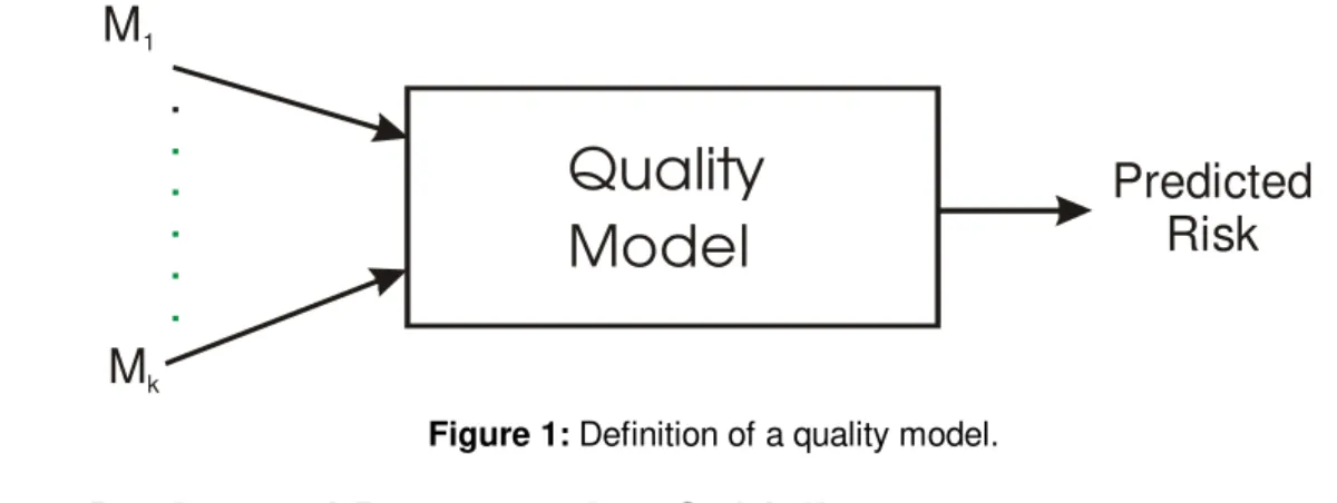
Predicting whether a component is high risk or not is achieved through a quality model. A quality model is a quantitative model that can be used to:

• Predict which components will be high risk. For example, some quality models make binary predictions as to whether a component is faulty or not-faulty [11][30][31][35][75][82].

• Rank components by their risk-proneness (in whatever way risk is defined). For instance, there have been studies that predict the number of faults in individual components (e.g., [72]), and that

produce point estimates of maintenance effort (e.g., [66][84]). These estimates can be used for ranking the components.

An overview of a quality model is shown in Figure 1. A quality model is developed using a statistical or machine learning modeling technique, or a combination of techniques. This is done using historical data. Once constructed, such a model takes as input the values on a set of metrics for a particular component (

M K

₁

M

_k), and produces a prediction of the risk (say either high or low risk) for that component.

A number of organizations have integrated quality models and modeling techniques into their overall quality decision making process. For example, Lyu et al. [87] report on a prototype system to support developers with software quality models, and the EMERALD system is reportedly routinely used for risk assessment at Nortel [60][61]. Ebert and Liedtke describe the application of quality models to control the quality of switching software at Alcatel [27].

Quality

Model

. . . . . .

M

1

M

k

Predicted

Risk

Figure 1: Definition of a quality model.

3.2

Design and Programming Guidelines

An appealing operational approach for constructing design and programming guidelines using software product metrics is to make an analogy with conventional statistical quality control: identify the range of values that are acceptable or unacceptable, and take action for the components with unacceptable values [79]. This means identifying thresholds on the software product metrics that delineate between ‘acceptable’ and ‘unacceptable’. In summarizing their experiences using software product measures, Szentes and Gras [115] state “the complexity measures of modules may serve as a useful ‘early warning’ system against poorly written programs and program designs. .... Software complexity metrics can be used to pinpoint badly written program code or program designs when the values exceed predefined maxima or minima.” They then argue that such thresholds can be defined subjectively based on experience. In addition to being useful during development, Coallier et al. [22] present a number of thresholds for procedural measures that Bell Canada uses for risk assessment during the acquisition of software products. The authors note that their thresholds identify 2 to 3 percent of all the procedures and classes for manual examination. Instead of experiential thresholds, some authors suggest the use of percentiles for this purpose. For example, Lewis and Henry [83] describe a system that uses percentiles on procedural measures to identify potentially problematic procedures. Kitchenham and Linkman [79] suggest using the 75th percentile as a cut-off value. More sophisticated approaches include identifying multiple thresholds simultaneously, such as in [1][5].

In an object-oriented context, thresholds have been similarly defined by Lorenz and Kidd as [86] “heuristic values used to set ranges of desirable and undesirable metric values for measured software.” Henderson-Sellers [54] emphasizes the practical utility of object-oriented metric thresholds by stating that “An alarm would occur whenever the value of a specific internal metric exceeded some predetermined threshold.” Lorenz and Kidd [86] present a number of thresholds for object-oriented metrics based on their experiences with Smalltalk and C++ projects. Similarly, Rosenberg et al. [102] have developed thresholds for a number of popular object-oriented metrics that are used for quality management at NASA GSFC. French [42] describes a technique for deriving thresholds, and applies it to metrics collected from Ada95 and C++ programs. Chidamber et al. [21] state that the premise behind managerial use of object-oriented metrics is that extreme (outlying) values signal the presence of high complexity that may require management action. They then define a lower bound for thresholds at the 80th percentile (i.e., at most 20% of the observations are considered to be above the threshold). The authors note that this is consistent with the common Pareto (80/20) heuristic.

3.3

Making System Level Predictions

Typically, software product metrics are collected on individual components for a single system. Predictions on individual components can then be aggregated to give overall system level predictions. For example, in two recent studies using object-oriented metrics, the authors predicted the proportion of faulty classes in a whole system [31][46]. This is an example of using predictions of fault-proneness for each class to draw conclusions about the overall quality of a system. One can also build prediction models of the total number of faults and fault density [36]. Similarly, another study used object-oriented metrics to predict the effort to develop each class, and these were then aggregated to produce an overall estimate of the whole system’s development cost [16].

4 A Metrics Validation Methodology

The methodology that is described here is based on actual experiences, within software engineering and other disciplines where validation of measures is a common endeavor. The presentation below is intended to practical, in that we explain how to perform a validation and what are the issues that arise that must be dealt with. We provide guidance on the most appropriate ways to address common difficulties. In many instances we present a number of reasonable methodological options, discuss their advantages and disadvantages, and conclude by making a recommendation.

We will assume that the data analysis technique will be statistical, and will be a form of regression, e.g., logistic regression, or ordinary least squares regression. Many of the issues that are raised are applicable to other analysis techniques, in particular, machine learning techniques such as classification and regression trees; but not all. We focus on statistical techniques.

4.1

Overview of Methodology

The complete validation methodology is summarized below, with references to the relevant sections where each step is discussed. As can be seen, we have divided the methodology into three phases, planning, modeling, and post modeling. While the methodology is presented as a sequence of steps, in reality it is rarely a sequence of steps, and there is frequent iteration. We also assume that the analyst has a set of product metrics that need to be validated, rather than only one. If the analyst wishes to validate only one metric then the section below on variable selection would not be applicable.

Planning

Measurement of Dependent Variable Section 4.3

Selection of Data Analysis Technique Section 4.4

Model Specification Section 4.5

Specifying Train and Test Data Sets Section 4.6 Statistical Modeling

Model Building Section 4.7

Evaluating the Validity of a Product Metric Section 4.8

Variable Selection Section 4.9

Building and Evaluating a Prediction Model Section 4.10

Making System Level Predictions Section 4.11

Post Modeling

Interpreting Results Section 4.12

Reporting the Results of a Validation Study Section 4.13

4.2

Theoretical Justification

The reason why software product metrics can be potentially useful for identifying high risk components, developing design and programming guidelines, and making system level predictions is exemplified by the following justification for a product metric validity study “There is a clear intuitive basis for believing that complex programs have more faults in them than simple programs” [94]. In general, however, there has not been a strong theoretical basis driving the development of traditional software product metrics. Specifically, Kearney et al. [68] state that “One of the reasons that the development of software complexity measures is so difficult is that programming behaviors are poorly understood. A behavior must be understood before what makes it difficult can be determined. To clearly state what is to be measured,

we need a theory of programming that includes models of the program, the programmer, the programming environment, and the programming task.”

A theory is frequently stated at an abstract level, relating internal product attributes with external attributes. In addition, a theory should specify the mechanism which explains why such relationships should exist. To operationalize a theory and test it empirically the abstract attributes have to be converted to actual metrics. For example, consider Parnas' theory about design [96] which states that high cohesion within modules and low coupling across modules are desirable design attributes, in that a software system designed accordingly is easier to understand, modify, and maintain. In this case, it is necessary to operationally define coupling, understandability, modifiability, and maintainability into actual metrics in order to test the theory.

Recently, an initial theoretical basis for developing quantitative models relating product metrics and external quality metrics has been provided in [15], and is summarized in Figure 2. There, it is hypothesized that the internal attributes of a software component (i.e., structural properties), such as its coupling, have an impact on its cognitive complexity. Cognitive complexity is defined as the mental burden of the individuals who have to deal with the component, for example, the developers, testers, inspectors, and maintainers. High cognitive complexity leads to a component exhibiting undesirable external qualities, such as increased fault-proneness and reduced maintainability. Further detailed elaboration of this model has been recently made [32].

Internal Attributes (e.g., coupling) Cognitive Complexity External Attributes (e.g., fault-proneness, maintainability) affect affect indicate

Figure 2: Theoretical basis for the development of object oriented product metrics.

Hatton has extended this general theory to include a mechanism for thresholds. He argues that Miller [90] shows that humans can cope with around 7 +/- 2 pieces of information (or chunks) at a time in short-term memory, independent of information content. He then refers to [56], where they note that the contents of long-term memory are in a coded form and the recovery codes may get scrambled under some conditions. Short-term memory incorporates a rehearsal buffer that continuously refreshes itself. He suggests that anything that can fit into short-term memory is easier to understand. Pieces that are too large or too complex overflow, involving use of the more error-prone recovery code mechanism used for long-term storage. In a subsequent article, Hatton [53] also extends this model to object-oriented development. Based on this argument, one can hypothesize threshold effects for many contemporary product metrics. El Emam has elaborated on this mechanism for object-oriented metrics [32].

It must be recognized that the above cognitive theory suggests only one possible mechanism of what would impact external metrics. Other mechanisms can play an important role as well. For example, some studies showed that software engineers experiencing high levels of mental and physical stress tend to produce more faults [43][44]. Mental stress may be induced by reducing schedules and changes in requirements. Physical stress may be a temporary illness, such as a cold. Therefore, cognitive complexity due to structural properties, as measured by product metrics, can never be the reason for all faults. However, it is not known whether the influence of software product metrics dominates other effects. The only thing that can reasonably be stated is that the empirical relationships between software product metrics and external metrics are not very likely to be strong because there are other effects that are not accounted for, but as has been demonstrated in a number of studies, they can still be useful in practice.

4.3

Measurement of Dependent Variables

In software product metric validation continuous variables are frequently counts. A count is characterized by being a non-negative integer, and hence is a discrete variable. It can be, for example, the number of faults found in the component or the effort to develop the component2. One can conceivably construct a variable such as fault density (number of faults divided by size), which is neither of the above. However, in such cases it is more appropriate to have size as an independent variable in a validation model and have the number of defects as the dependent variable.3

Binary variables are typically not naturally binary. For example, it is common for the analyst to designate components that have no faults as not-faulty and those that have a fault as faulty. This results in a binary variable. Another approach that is used is to dichotomize a continuous dependent variable around the median [29], or even on the third quartile [74].

4.3.1 Dichotomizing Continuous Variables

In principle, dichotomizing a continuous variable results in the loss of information in that the continuous variable is demoted to a binary one. Conceivably, then, validation studies using such a dichotomization are weaker, although it has not been demonstrated in a validation context how much weaker (it is plausible that in almost all situations the same conclusions will be drawn).

Generally, it is recommended that when the dependent variable is naturally continuous, that it remains as such and not be dichotomized. This will alleviate any lingering doubts that perhaps the results would have been different had no dichotomization been performed. The only reasonable exception in favor of using binary variables is related to the reliability of data collection for the system being studied. We will illustrate this through a scenario.

Component Fault Problem

Report Failure

1 n

n 1

n n

Figure 3: ER model showing a possible relationship between failures and components. The acronym PR stands for Problem Report.

In many organizations whenever a failure is observed (through testing or from a customer) a Problem Report (PR) is opened. It is useful to distinguish between a failure and a failure instance. Consider Figure 3. This shows that each failure instance may be associated with only a single PR, but that a PR can be associated with multiple failure instances. Multiple failure instances may be the same failure, but detected by multiple users, and hence they would all be matched to a single PR. A fault occurs in a single component, and each component may have multiple faults. A PR can be associated with multiple faults, possibly in the same component or across multiple components.

Counting inaccuracies may occur when a PR is associated with multiple faults in the same component. For example, say because of schedule pressures, the developers fix all faults due to the same PR at the same time in one delta. Therefore, when data is extracted from a version control system it appears as one fault. Furthermore, it is not uncommon for developers to fix multiple faults due to multiple PRs in the same delta. In such a case it is not known how many faults were actually fixed since each PR may have been associated to multiple faults itself.

The above scenarios illustrate that, unless the data collection system is fine grained and followed systematically, one can reliably say that there was at least one fault, but not the exact number of faults that were fixed per component. This makes an argument for using a binary variable such as faulty/not-faulty.

2

Although effort in principle is not a discrete count, in practice it is measured as such. For example, one can measure effort at the granularity of minutes or hours.

3

4.3.2 Surrogate Measures

Some studies use surrogate measures. Good examples are a series of studies that used code churn as a surrogate measure of maintenance effort [55][84][85]. Code churn is the number of lines added, deleted, and modified in the source code to make a change. It is not clear whether code churn is a good measure of maintenance effort. Some difficult changes that consume a large amount of effort to make may result in very few changes in terms of LOC. For example, when performing corrective maintenance one may consume a considerable amount of time attempting to isolate the cause of the defect, such as when tracking down a stray pointer in a C program. Alternatively, making the fix may consume a considerable amount of effort, such as when dealing with rounding off errors in mathematical computations (this may necessitate the use of different algorithms altogether which need to be implemented). Furthermore, some changes that add a large amount of code may require very little effort (e.g., cloning error-checking functionality from another component, or deletion of unused code). One study of this issue is presented in the appendix (Section 6). The results suggest that using code churn as a surrogate measure of maintenance effort is not strongly justifiable, and that it is better not to follow this practice.

Therefore, in summary, the dependent variable ought not to be dichotomized unless there is a compelling reason to do so. Furthermore, analysts should be discouraged from using surrogate measures, such as code churn, unless there is evidence that they are indeed good surrogates.

4.4

Selection of Data Analysis Technique

The selection of a data analysis technique is a direct consequence of the type of the dependent variable that one is using. In the discussion that follows we shall denote the dependent variable by

y

and the independent variables by

x

_i.

4.4.1 A Binary Dependent Variable

If

y

is binary, then one can construct a logistic regression (LR) model. The form of a LR model is:

        + −

∑

+

=

= k i i ix

e

1 0

1

1

β β

π

Eqn. 1

where

π

is the probability of a component being high-risk, and the

x

i’s are the independent variables.

The

β

parameters are estimated through the maximization of a log-likelihood [59]. 4.4.2 A Continuous Dependent Variable That is Not a Count

As noted earlier, a continuous may or may not be a count variable. If

y

is not a count variable, then one can use the traditional ordinary least squares (OLS) regression model4. The OLS model takes the form:

∑

+

=

= k i i i

x

y

1 0

β

β

Eqn. 2

4.4.3 A Continuous Dependent Variable That is a Count

If

y

is a (discrete) count variable, such as the number of faults or development effort, it may seem that a straight forward approach is to also build an OLS model as in Eqn. 2. This is not the case.

In principle, using an OLS model is problematic. First, an OLS model can predict negative values for faults or effort, and this is clearly meaningless. For instance, this is illustrated in Figure 4, which shows the relationship between the number of methods (NM) in a class and the number of post-release faults for the Java system described in [46] as calculated using OLS regression. As can seen, if this model is used

4

to predict the number of faults for a class with two methods the number of faults predicted will be negative. NM N u m b e r o f F a u lts 0 5 10 0 10 20 30 40 50 60 70 80 90

Figure 4: Relationship between the number of methods in a class and the number of faults.

Furthermore, such count variables are decidedly non-normal, violating one of the assumptions used in deriving statistical tests for OLS regression. Marked heteroscedasticity is also likely which can affect the standard errors: they will be smaller than their true value, and therefore t-tests for the regression coefficients will be inflated [45]. King [77] notes that these problems lead to coefficients that have the wrong size and may even have the wrong sign.

Taking the logarithm of

y

may alleviate some of these problems of the OLS model. Since

y

can have zero values, one can add a small constant, typically 0.01 or 0.5:

log

(

y

+

c

)

[77]. An alternative is to take the square root of

y

[65][77]. The square root transformation, however, would result in an awkward model to interpret. With these transformations it is still possible to obtain negative predictions. This creates particular problems when the square root transformation is used. For example, Figure 5 shows the relationship between NM and the square root of faults for the same system. In a prediction context, this OLS model can predict negative square root number of faults for very small classes.

WMC s q rt(N u m b e r o f F a u lts ) 0 1 2 3 4 5 0 10 20 30 40 50 60 70 80 90

Also, in many cases the resulting distribution still has its mode5 at or near the minimal value after such transformations. For example, Figure 6 shows the original fault counts found during acceptance testing for one large system described in [35].6 As can be seen, the mode is still at the minimal value even after the logarithmic or square root transformation. Another difficulty with such transformations occurs when making system level predictions. The Jensen inequality (see [112]) states for a convex function

g

( y

)

that

E

(

g

( )

y

)

≥

g

(

E

( )

y

)

. Given that the estimates from OLS are expected values conditional on the

x

values, for the above transformations the estimates produced from the OLS regression will be systematically biased.

In addition, when

y

is a count of faults, an OLS model makes the unrealistic assumption that the difference between no faults and one fault is the same as the difference between say 10 faults and 11 faults. In practice, one would reasonably expect a number of different effects:

• The probability of a fault increases as more faults are found. This would mean that there is an intrinsic problem with the design and implementation of a component and therefore the incidence of a fault is an indicator that there are likely to be more faults. Furthermore, one can argue that as more fixes are applied to a component, new faults are introduced by the fixes and therefore the probability of finding a subsequent fault increases. Evidence of this was presented in a recent study [9] whereby it was observed that components with more faults pre-release also tend to have more faults post-release, leading to the conclusion that the number of faults already found is positively related of the number of faults to be found in the future. This is termed positive

contagion.

• The probability of a fault decreases as more faults are found. This would be based on the argument that there are a fixed number of faults in a component and finding a fault means that there are fewer faults left to find and these are likely to be the more difficult ones to detect. This is termed negative contagion.

5

The mode is the most frequent category [121].

6

In the study described in [35] only a subset of the data was used for analysis. The histograms shown in Figure 6 are based on the complete data set consisting of 11012 components.

0 10 20 30 40 0 2 0 0 0 4 0 0 0 6 0 0 0 8 0 0 0 1 0 0 0 0 NFaults 0 1 2 3 0 2 0 0 0 4 0 0 0 6 0 0 0 8 0 0 0 log(NFaults+0.5) 0 1 2 3 4 5 6 0 2 0 0 0 4 0 0 0 6 0 0 0 8 0 0 0 sqrt(NFaults)

Figure 6: The effect of different transformations of the number of faults dependent variable. The x-axis shows the value of faults or transformed faults, and the y-axis shows the frequency.

A more principled approach is to treat the

y

variable as coming from a Poisson distribution, and perform a Poisson regression (PR) [123]. For example, Evanco presents a Poisson model to predict the number of faults in Ada programs [36], and Briand and Wuest use Poisson models to predict development effort for object-oriented applications [16].

One can argue that when the

y

values are almost all large the Poisson distribution becomes approximately normal, suggesting that if the Poisson distribution is appropriate for modeling the count variable, then OLS regression will do fine. King [77] defined large as being almost every observation having a count greater than 30. This is unlikely to be true for fault counts, and for effort Briand and Wuest [16] have made the explicit point that large effort values are rare.

A Poisson distribution assumes that the variance is equal to the mean – equidispersion. At least for object-oriented metrics and development effort, a recent study has found overdispersion [16] – the variance is larger than the mean. Parameter estimates when there is overdispersion are known to be inefficient and the standard errors are biased downwards [19]. Furthermore, the Poisson distribution is non-contagious, and therefore would not be an appropriate model, a priori, for fault counts.

The negative binomial distribution allows for overdispersion, hence the conditional variance can be larger than the conditional mean in a negative binomial regression (NBR) model. Furthermore, NBR can model positive contagion. An important question is whether dependent variables better fit a negative binomial distribution or a Poisson distribution. To answer this question we used the number of faults data for all 11012 components in the procedural system described in [35], and the 250 classes for the object-oriented system described in [46]. Using the actual data set, maximum likelihood estimates were derived for a Poisson and a negative binomial distribution, and then these were used as starting values in a Levenberg-Marquardt optimization algorithm [100] to find the distribution parameters that best fit the data, optimizing on a chi-square goodness-of-fit test. The actual data sets were then compared to these optimal distributions using a chi-square test. In both cases the results indicate that the negative binomial distribution is a better fit to the fault counts than the Poisson distribution. Therefore, at least based on this

initial evaluation, one may conclude that NBR models would be more appropriate than Poisson regression models for fault counts.

Type of

Dependent

Variable

Binary

Continuous

Logistic

Regression

_Variable

Count

Yes

No

Dependent

Measure

OLS

Regression

Faults

Effort

NB Regression

or

GEC

Truncated at Zero

NB Regression

Figure 7: Decision tree for selecting an analysis method. The non-terminal nodes are conditions. Each arc is labeled with the particular value for the condition. Terminal nodes are the recommended analysis

technique(s).

NBR would still have deficiencies for modeling faults since it does not allow for the possibility of negative contagion. A general event count (GEC) model that accommodates both types of contagion has been presented in [78]. Until there is a clearer understanding of how the incidence of a fault affects the incidence of another fault, one should use both modeling approaches and compare results: the NBR and the GEC.

In the case of development effort data, it is meaningless to have an effort value of zero. However the NBR model assumes that zero counts exist. To alleviate this, truncated-at-zero NBR is the most appropriate modeling technique [123]. This assumes that counts start from one.

Two simulation studies provide further guidance about the appropriate modeling techniques to use. One simulation using a logarithmic transformation of a count

y

and OLS regression found that this produced biased coefficient estimates, even for large samples [77]. It was also noted that the estimates were not consistent, and that the Poisson regression model generally performed better. Another Monte Carlo simulation [114] found that the Type I error rates7 of the PR model were disturbingly large; the OLS

7

regression model with and without a square root transformation yielded Type I error rates almost equal to what would be expected by chance; and that the negative binomial model also had error rates equal to the nominal level. Even though the second simulation seems encouraging for OLS regression models, they would still not be advisable because of their inability to provide unbiased system level predictions and due to the possibility of giving negative predictions. The PR model is not recommended based on the arguments cited above as well as the inflated Type I error rate. It would therefore be reasonable to use at least the NBR model for validating product metrics when the

y

variable is a fault count, and ideally the community should investigate the utility of the additional modeling of negative contagion through the GEC.

The above exposition has attempted to provide clear guidance and justifications for the appropriate models to use, in principle. We have summarized these guidelines in the decision tree of Figure 7. Admittedly, if one were to look at the software product metrics validation literature today, one would see a predominant use of OLS regression and LR.

4.5

Model Specification

When using a statistical technique it is necessary to specify the model a priori (this is not the case for many machine learning techniques). Model specification involves making five decisions on:

• Whether to use principal components.

• The functional form of the relationship between the product metrics and the dependent variable.

• Modeling interactions.

• Which confounding variables to include.

• Examination of thresholds.

4.5.1 The Use of Principal Components

Principal components analysis (PCA) [76] is a data reduction technique that can be used to reduce the number of product metrics. Therefore, if one has

k

product metrics, PCA will group them into

z

orthogonal dimensions such that

z

<

k

where all the metrics within each dimension are highly correlated amongst themselves but have relatively small correlations with metrics in a different dimension. The logic is that each dimension represents a single underlying construct that is responsible for the observed correlations [93].

Once the dimensions are identified, there are typically two ways to produce a single metric for each dimension. The first is to sum the metrics within each dimension. The second is to use a weighted sum. The latter are often referred to as “domain metrics” [73]. Instead of using the actual metrics during validation, one can then use the domain metrics, as was done, for example, in [73][82]. The advantage of this approach is that it practically eliminates the problem of collinearity (discussed below).

Domain metrics have some nontrivial disadvantages as well. First, some studies report that there is no difference in the accuracy of a model using domain metrics versus the original metrics [82]. Another study [69] concluded that principal components are unstable across different products in different organizations. This suggests that the definition of a domain metric will be different across studies, making the accumulation of knowledge about product metrics rather tenuous. Furthermore, as noted in [40], such domain metrics are difficult to interpret and act upon by practitioners.

In general, the use of principal components or domain metrics as variables in models is not advised. In addition to the above disadvantages, there are other ways of dealing with multicollinearity, therefore there is no compelling reason for using domain metrics.

4.5.2 Specifying the Functional Form

It is common practice in software engineering validation studies to assume a linear relationship between the product metrics and the dependent variable. However, this is not always the best approach. Most product metrics are counts, and they tend to have a skewed distribution, which can be characterized as lognormal (or more appropriately negative binomial since the counts are discrete). This presents a

problem in practice in that many analysis techniques assume a normal distribution, and therefore just using the product metric as it is would be considered a violation of the assumptions of the modeling technique. To remedy this it is advisable to perform a transformation on the product metrics, typically a logarithmic transformation will be adequate. Since with product metrics there will be cases with values of zero, it is common to take

log

(

x

_i

+

0

.

5

)

. Taking the logarithm will also in many instances linearize the relationship between the product metrics and the dependent variable. For example, if one is building a LR model with a metric

M

and size

S

, then the model can be specified as:

( M S)

e

− + ′+ ′

+

=

2 1 0

1

1

β β β

π

Eqn. 3

where

M

′

=

log

(

M

+

0

.

5

)

and

S

′

=

log

(

S

+

0

.

5

)

. In practice, it is advised that a pair of models with transformed and untransformed variables are built, and then the results can be compared. Alternatively, a more principled approach is to check for the linearity assumption and to identify appropriate transformations that can be followed, such as the alternating conditional expectation algorithm for OLS regression which attempts to find appropriate transformations [10] (also see [120] for a description of how to use this algorithm to decide on transformations), and partial residual plots for LR [81].

4.5.3 Specifying Interactions

It is not common in software engineering validation studies to consider interactions. An interaction specifies that the impact of one independent variable depends on the level of the other independent variable. To some extent this is justified since there is no strong theory predicting interaction effects. However, it is also advisable to at least consider models with interactions and see if the interaction variable is statistically significant. If it is not then it is safe to assume that there are no interactions. If it is, then interactions must be included in the model specification. When there are many product metrics to consider the number of possible interactions can be very large. In such cases, it is also possible to use a machine learning technique to identify possible interactions, and then only include the interactions identified by the machine learning technique. A typical way for specifying interactions is to add a multiplicative term: ( M S MS)

e

− + ′+ ′+ ′′

+

=

3 2 1 0

1

1

β β β β

π

Eqn. 4

If the interaction coefficient,

β

₃, is statistically significant, then this indicates that there is an interaction effect.

4.5.4 Including Confounding Variables in the Specification

It is also absolutely critical to include potential confounding variables as additional independent variables when validating a product metric. A confounding variable can distort the relationship between the product metric and the dependent variable. One can easily control for confounding variables by including them as additional variables in the regression model.

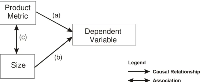
A recent study [34] has demonstrated a confounding effect of class size on the validity of object-oriented metrics. This means that if one does not control the effect of class size when validating metrics, then the results would be quite optimistic. The reason for this is illustrated in Figure 8. Size is correlated with most product metrics (path (c)), and it is also a good predictor of most dependent variables (e.g., bigger components are more likely to have a fault and more likely to take more effort to develop – path (b)). For example, there is evidence that object-oriented product metrics are associated with size. In [18] the Spearman rho correlation coefficients go as high as 0.43 for associations between some coupling and cohesion metrics with size, and 0.397 for inheritance metrics, and both are statistically significant (at an alpha level of say 0.1). Similar patterns emerge in the study reported in [15], where relatively large correlations are shown. In another study [20] the authors display the correlation matrix showing the Spearman correlation between a set of object-oriented metrics that can be collected from Shlaer-Mellor designs and C++ LOC. The correlations range from 0.563 to 0.968, all statistically significant at an alpha

level 0.05. This also indicates very strong correlations with size. The relationship between size and faults is clearly visible in the study of [20], where the Spearman correlation was found to be 0.759 and statistically significant. Another study of image analysis programs written in C++ found a Spearman correlation of 0.53 between size in LOC and the number of faults found during testing [50], and was statistically significant at an alpha level of 0.05. Briand et al. [18] find statistically significant associations between 6 different size metrics and fault-proneness for C++ programs, with a change in odds ratio going as high as 4.952 for one of the size metrics.

Therefore, if an association is found between a particular metric and the dependent variable, this may be due to the fact that higher values on that metric also mean higher size values. Inclusion of size in the regression model, as we did in Eqn. 3, is straight-forward. This allows for a statistical; adjustment of the effect of size. It is common that validation studies do not control for size. For object-oriented metrics, validation studies that did not control for size include [8][15][18][51][116]. It is not possible to draw strong conclusions from such studies.

Product

Metric

Dependent

Variable

Size

(a)

(b)

(c)

Figure 8: Illustration of counfounding effect of class size.

Therefore, in summary it is necessary to adjust for confounding variables. While there are many potential confounders, size at a minimum must be controlled since it is easy to collect in a metrics validation study. Other confounding variables are discussed in Section 5.

4.5.5 Specifying Thresholds

Given the practical and theoretical implications of thresholds, it is also important to evaluate thresholds for the product metrics being validated. In the case of a LR model, a threshold can be defined as [119]:

(

) (

)

(

β β β τ τ

)

π

_{− + + − −} +

+

=

_{S M I M}

e

0 1 2

1

1

Eqn. 5 where:

( )







>

≤

=

+

0

1

0

0

z

if

z

if

z

I

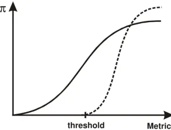
Eqn. 6

A recent study [33] has shown that there are no size thresholds for object-oriented systems. Therefore size can be kept as a continuous variable in the model. However, this is not a foregone conclusion, and further studies need to verify this for object-oriented and procedural systems.

The difference between the no threshold and threshold model is illustrated in Figure 9. For the threshold model the probability of a being high risk only starts to increase once the metric is greater than the threshold value,

τ

.

Metric

π

threshold

Figure 9: Relationship between the metric M and the probability of being high risk for the threshold and no threshold models. This is the bivariate relationship assuming size is kept constant.

To estimate the threshold value,

τ

, one can maximize the log-likelihood for the model in Eqn. 5. Ulm [119] presents an algorithm for performing this maximization.

Once a threshold is estimated, it should be evaluated. This is done by comparing the no-threshold model with the threshold model. Such a comparison is, as is typical, done using a likelihood ratio statistic (for example see [59]). The null hypothesis being tested is:

) 1 (

0

:

M

H

τ

≤

_{Eqn. 7}

where

M

(1) is the smallest value for the measure

M

in the data set. If this null hypothesis is not rejected then it means that the threshold is equal to or below the minimal value. When the product metric is a count, this is exactly like saying that the threshold model is the same as the no-threshold model. Hence one can conclude that there is no threshold. The alternative hypothesis is:

) 1 (

1

:

M

H

τ

>

_{Eqn. 8}

which would indicate that a threshold effect exists. In principle, one can also specify models with thresholds for multiple product metrics and using other regression techniques.

4.6

Specifying Train and Test Data Sets

Although the issue of train and test data sets becomes important during the construction and evaluation of prediction models (see Section 4.10), it must be decided upon at the early stages of metrics validation. It is known that if an analyst builds a prediction model on one data set and evaluates its prediction accuracy on the same data set, then the accuracy will be artificially inflated. This means that the accuracy results obtained during the evaluation will not generalize when the model is used on subsequent data sets, for example, a new system. Therefore, the purpose of deciding on train and test sets is to come up with a strategy that will allow the evaluation of accuracy in a generalizeable way.

If the analyst has two data sets from subsequent releases of a particular system, then the earliest release can be designated as the training data set, and the later release as the test data set. If there are more than two releases, then the analyst could evaluate the prediction model on multiple test sets. Sometimes data sets from multiple systems are available. In such cases one of the data sets is designated as the training data set (usually the one with the largest number of observations) and the remaining system data sets as the test sets.

If the analyst has data on one system, then a common strategy that is used is to randomly split the data set into a train and a test set. For example, randomly select one third of the observations as the test set and the remaining two thirds is your training set. All model building is performed on the training data set. Evaluation of accuracy is then performed by comparing the predicted values from the model to the actual values in the test set.

Another approach is to use cross-validation. There are two forms of cross-validation: leave-one-out and k-fold cross-validation. In leave-one-out cross-validation the analyst removes one observation from the data set, builds a model with the remaining

n

−

1

observations, and evaluates how well the model predicts the value of the observation that is removed. This process is repeated each time removing a different observation. Therefore, one builds and evaluates

n

models. With k-fold cross-validation the analyst randomly splits the data set into k approximately equally sized groups of observations. A model is built using k-1 groups and its predictions evaluated on the last group. This process is repeated each time by removing a different group. So for example if k is ten, then 10 models are constructed and validated. Finally, a more recent approach that has been used is called bootstrapping [28]. A training set is constructed by sampling with replacement. Each sample consists of

n

observations from the data set, where the data set has

n

observations. Some of the observations may therefore be duplicates. The remaining observations that were not sampled at all are the test set. A model is built with the training set and evaluated on the test set. This whole process is repeated say 500 times, each time sampling with replacement

n

observations. Therefore one builds and evaluates 500 models.

In general, if one’s data set is large (say more than 200 observations), then one can construct a train and test set through random splits. If the data set is smaller than that, one set of recommendations for selecting amongst these alternatives has been provided in [122]:

• For sample sizes greater than 100, use validation, leave-one-out or 10-fold cross-validation.

• For sample sizes less than 100, use leave-one cross validation

• For sample sizes that are less than 50 one can use either the bootstrap approach or the leave-one-out approach.

There are alternative strategies that can be used, and these are discussed in [122]. However, at least in the software product metrics, the above are the most commonly seen approaches.

4.7

Model Building

During the construction of models to validate metrics, it is necessary to pay attention to issues of model stability and evaluating the goodness-of-fit of the model.

4.7.1 Model Building Strategy

A general strategy for model building consists of two stages. The first is to develop a model with each metric and the confounders. This model will allow the analyst to determine which metrics are related to the dependent variable (see Section 4.8). Recall that building a model without confounders does not provide useful information and therefore should be avoided. In the second stage a subset of the metrics that are related with the dependent variable are selected to build a prediction model. Variable selection is discussed in 4.9 and evaluating the prediction model is discussed in 4.10.

Below we present some of the important issues that arise when building a model, in either of the above stages.

4.7.2 Diagnosing Collinearity

One of the requirements for properly interpreting regression models is that no one of the independent variables are perfectly linearly correlated to one or more other independent variables. Perfect linear correlation is referred to as perfect collinearity. When there is perfect collinearity then the regression surface is not even defined. Perfect collinearity is rare, however, and therefore one talks about the

degree of collinearity. Recall that confounders are associated with the product metric by definition, and

therefore one should not be surprised if strong collinearity exists. The larger the collinearity, the greater the standard errors of the coefficient estimates. One implication of this is that the conclusions drawn about the relative impacts of the independent variables based on the regression coefficient estimates from the sample are less stable.

A commonly used diagnostic to evaluate the extent of collinearity is the condition number [6][7]. If the condition number is larger than a threshold, typically 30, then one can conclude that there exists severe collinearity and remedial actions ought to be taken. One possible remedy is to use ridge regression techniques. Ridge regression has been defined for OLS models [57][58], and extended for LR models [104][105].

4.7.3 Influential Observations

Influence analysis is performed to identify influential observations (i.e., ones that have a large influence on the regression model). This can be achieved through deletion diagnostics. For a data set with

n

observations, estimated coefficients are recomputed

n

times, each time deleting exactly one of the observations from the model fitting process. For OLS regression, a common diagnostic to detect influential observations is Cook’s distance [24][25]. For logistic regression, one can use Pergibon’s

∆

β

diagnostic [97].

It should be noted that an outlier is not necessarily an influential observation [103]. Therefore, approaches such as those described in [18] for identifying outliers in multivariate models will not necessarily identify influential observations. Specifically, they [18] use the Mahalanobis distance from the centroid, removing each observation in turn before computing the centroid. This approach has some deficiencies. For example, an observation may be further away from the other observations but may be right on the regression surface. Furthermore, influential observations may be clustered in groups. For example, if there are say two independent variables in our model and there are five out of the

n

observations that have exactly the same values on these two variables, then these 5 observations are a group. Now, assume that this group is multivariately different from all of the other

n

−

5

observations. Which one of these 5 would be considered an outlier ? A leave-one-out approach may not even identify any one of these observations as being different from the rest since in each run the remaining 4 observations will be included in computing the centroid. Such masking effects are demonstrated in [6].

The identification of outliers is useful, for example, when interpreting the results of logistic regression: the estimate of the change in odds ratio depends on the sample standard deviation of the variable. If the standard deviation is inflated due to outliers then you will also get an inflated change in odds ratio.

When an influential observation or an outlier is detected, it would be prudent to inspect that observation to find out why it is problematic rather than just discarding it. It may be due to a data entry error, and fixing that error results in retaining the observation.

4.7.4 Goodness of fit

Once the model is constructed it is useful to evaluate its goodness-of-fit. Commonly used measures of goodness-of-fit are R2 for OLS and pseudo-R2 measures of logistic regression. While R2 has a straight-forward interpretation in the context of OLS, for logistic regression this is far from the case. Pseudo-R2 measures of logistic regression tend to be small in comparison to their OLS cousins. Menard gives a useful overview of the different pseudo-R2 coefficients that have been proposed [88], and recommends the one described by Hosmer and Lemeshow [59].

4.8

Evaluating the Validity of a Product Metric

The first step in validating a metric is to examine the relationship between the product metric and the dependent variable after controlling for confounding effects. The only reason for building models that do not control for confounding effects is to see how big the confounding effect is. In such a case one would build a model without the confounding variable, and a model with the confounding variable, and see how much the estimated parameter for the product metric changes. However, models without confounder control do not really tell us very much about the validity of the metric.

There are two aspects to the relationship between a product metric and the dependent variable: statistical significance and the magnitude of the relationship. Both are important, and both concern the estimated parameters in the regression models. Statistical significance tells us the probability of getting an estimated parameter as large as the one actually obtained if the true parameter was zero.8 If this probability is larger than say 0.05 or 0.1, then we can have confidence that it is larger than zero. The magnitude of the parameter tells us how much influence the product metric has on the dependent variable. The above two are not necessarily congruent. It is possible to have a large parameter and no statistical significance. This is more likely to occur if the sample size is small. It is also possible to have a statistically significant parameter that is rather small. This is more likely to occur with large samples. Most parameters are interpretable by themselves. However, sometimes it is also useful to compare the parameters obtained by different metrics. Direct comparison of regression parameters is incorrect because the product metrics are typically measured on different units. Therefore, they need to be normalized. In ordinary least squares regression one would use

β =

i

′

σ

i

β

i, which measures the change

in the

y

variable when there is a one standard deviation change in the

x

i variable (the

σ

i value is the

standard deviation of the

x

i variable). In logistic regression one would use the change in odds ratio

given by

∆Ψ

=

_e

βiσi_{, which is interpreted as the change in odds by increasing the value of}

i

x

by one standard deviation. Such normalized measures are appropriate for comparing different parameters, and finding out which product metric has the biggest influence on the dependent variable.

Since most software engineering studies are small sample studies, if a metric’s parameter is found to be statistically significant, then it is considered to be “validated”. Below we discuss the interpretation of insignificant results (see Section 4.12).

4.9

Variable Selection

Now that we have number of validated metrics, we wish to determine whether we can build a useful prediction model. A useful prediction model should contain the minimal number of “best” validated metrics; the best being interpreted as the metrics that have the biggest impact on the dependent variable. For example, in the case of logistic regression, this will be the variable with the largest change in odds ratio. Finding the “best” metrics is typically not a simple determination since many product metrics are strongly correlated with each other. For example, it has been postulated that for procedural software, product metrics capture only five dimensions of program complexity [93]: control, volume (size), action, effort, and modularity. If most of the “best” metrics are correlated with each other or are measuring the same thing, a model incorporating the strongly correlated variables will not be stable due to high collinearity. Therefore, the metrics selected should also be orthogonal.

The first caution is that one ought not use automatic variable selection techniques to identify the “best” variables. There have been a number of studies that present compelling evidence that automatic selection techniques tend to have a large tendency to select “noise” variables, especially when the set of variables is highly correlated. This means that the final model with the automatically selected variables will not tell us which are the best metrics, and will likely be unstable in future data sets. For example, a Monte Carlo simulation of forward selection indicated that in the presence of collinearity amongst the independent variables, the proportion of ‘noise’ variables that are selected can reach as high as 74% [26].

8

In principle, other values than zero can be used. However, in software engineering studies testing for the zero value is almost universal.

It is clear that, for instance, in recent object-oriented metrics validation studies many of the metrics were correlated [15][18]. Harrell and Lee [48] note that when statistical significance is the sole criterion for including a variable the number of variables selected is a function of the sample size, and therefore tends to be unstable across studies. Furthermore, some general guidelines on the number of variables to consider in an automatic selection procedure for logistic regression are provided in [49]. Typically, software engineering studies include many metrics whose number is larger than those guidelines [15][18]. Therefore, the variables selected through such a procedure should not be construed as the best product metrics. In fact, automatic selection should only be considered as an exploratory technique whose results require further confirmation. Their use is not necessary though as easy alternatives can be used from which one can draw stronger conclusions.

If there are only a few metrics that have been found to be valid, then a simple correlation matrix would identify which metrics are strongly associated with each other. It is then easy to select a subset of metrics that both have the strongest relationship with the dependent variable and that have a weak correlation to each other.

If there are many validated metrics, one commonly used approach is to perform a principal components analysis [76]. The use of PCA for variable selection is different from its use for defining domain metrics discussed earlier (see Section 4.5.1). One can take the subset of metrics that are validated and perform a principal components analysis with them. The dimensions that are identified can then be used as the basis for selecting metrics. The analyst then selects one metric from each factor that is most strongly associated with the dependent variable.

4.10

Building and Evaluating a Prediction Model

Now that variables have been selected, one can develop a prediction model, following the guidelines above for model building. The prediction model must also include all the confounding variables considered earlier. Evaluation of the accuracy of the prediction model must follow. The approach for evaluation will depend on whether the analyst has only one data set or a train and test data set. These options were discussed above.

An important consideration is what coefficient to use to characterize prediction accuracy. A plethora of coefficients have been used in the software engineering literature. The coefficients differ depending on whether the dependent variable is binary or continuous and whether the predictions are binary or discrete.

4.10.1 Binary Dependent Variable and Binary Prediction

This situation occurs if the dependent variable is binary and the modeling technique that one is using makes binary predictions. For example, if one is using a classification tree algorithm, then the predictions are binary.

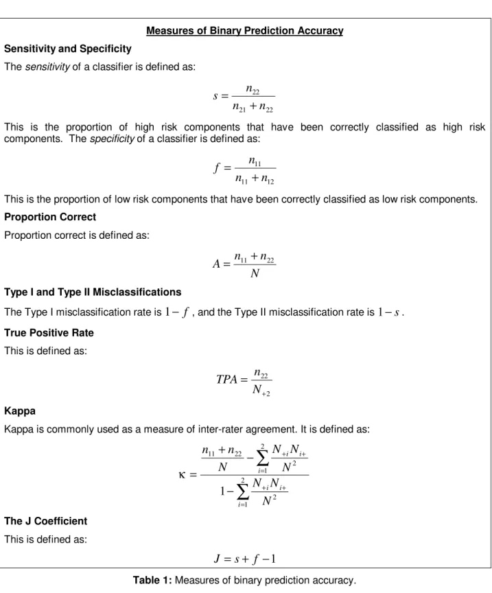
A plethora of coefficients have been used in the literature for evaluating binary predictions, for example, a chi-square test [1][5][82][108], sensitivity and specificity [1], proportion correct [1][82][107] (also called correctness in [98][99]), type I and type II misclassifications [70][71], true positive rate [11][15][18], and Kappa [15][18]. A recent comprehensive review of these measures [35] recommended that they should not be used as evaluative measures because either: (i) the results they produce depend on the proportion of high-risk components in the data set and therefore are not generalizeable except to other systems with the same proportion of high-risk components, or (ii) can only provide consistently unambiguous results if used in combination with other measures.

A commonly used notation for presenting the results of a binary accuracy evaluation is shown below (this is known as a confusion matrix).

Predicted Risk

Low High

Real Risk Low n11 n12 N1+

High n21 n22 N2+

N+1 N+2 N

A summary of all of the above measures is provided in Table 1 with reference to the notation in the above confusion matrix.