HAL Id: insu-02362729
https://hal-insu.archives-ouvertes.fr/insu-02362729
Submitted on 28 Nov 2020
HAL is a multi-disciplinary open access
archive for the deposit and dissemination of
sci-entific research documents, whether they are
pub-lished or not. The documents may come from
teaching and research institutions in France or
abroad, or from public or private research centers.
L’archive ouverte pluridisciplinaire HAL, est
destinée au dépôt et à la diffusion de documents
scientifiques de niveau recherche, publiés ou non,
émanant des établissements d’enseignement et de
recherche français ou étrangers, des laboratoires
publics ou privés.
67P/Churyumov–Gerasimenko near Perihelion as
Measured by Rosetta’s Alice Far-UV Spectrograph
Brian A. Keeney, S. Alan Stern, Ronald J. Vervack, Jr, Matthew M. Knight,
John Noonan, Joel Wm. Parker, Michael F. A’Hearn, Jean-Loup Bertaux,
Lori M. Feaga, Paul D. Feldman, et al.
To cite this version:
Brian A. Keeney, S. Alan Stern, Ronald J. Vervack, Jr, Matthew M. Knight, John Noonan, et al..
Upper Limits for Emissions in the Coma of Comet 67P/Churyumov–Gerasimenko near Perihelion as
Measured by Rosetta’s Alice Far-UV Spectrograph. Astronomical Journal, American Astronomical
Society, 2019, 158 (6), art. 252 (9p.). �insu-02362729�
Draft version November 5, 2019
Typeset using LATEX twocolumn style in AASTeX62
Upper Limits for Emissions in the Coma of Comet 67P/Churyumov-Gerasimenko Near Perihelion as Measured by Rosetta’s Alice Far-Ultraviolet Spectrograph
Brian A. Keeney,1 S. Alan Stern,1 Ronald J. Vervack, Jr.,2 Matthew M. Knight,3 John Noonan,4 Joel Wm. Parker,1 Michael F. A’Hearn,3,∗ Jean-Loup Bertaux,5 Lori M. Feaga,3 Paul D. Feldman,6 Richard A. Medina,1 Jon P. Pineau,7 Rebecca N. Schindhelm,1, 8 Andrew J. Steffl,1 M. Versteeg,9 and
Harold A. Weaver2
1Southwest Research Institute, Department of Space Studies, Suite 300, 1050 Walnut St., Boulder, CO 80302, USA
2Space Exploration Sector, Johns Hopkins University Applied Physics Laboratory, 11100 Johns Hopkins Rd., Laurel, MD 20723, USA 3Department of Astronomy, University of Maryland, College Park, MD 20742, USA
4Lunar and Planetary Laboratory, University of Arizona, 1629 E. University Blvd., Tucson, AZ 85721, USA 5LATMOS, CNRS/UVSQ/IPSL, 11 Boulevard d’Alembert, F-78280 Guyancourt, France
6Department of Physics and Astronomy, Johns Hopkins University, 3400 N. Charles St., Baltimore, MD 21218, USA 7Stellar Solutions, Inc., 250 Cambridge Ave., Suite 204, Palo Alto, CA 94306, USA
8Ball Aerospace and Technology Corp., 1600 Commerce St., Boulder, CO 80301, USA 9Southwest Research Institute, 6220 Culebra Rd., San Antonio, TX 78238, USA
ABSTRACT
The Alice far-UV imaging spectrograph (700-2050 Å) acquired over 70,000 spectral images during Rosetta’s 2-year escort mission, including over 20,000 in the months surrounding perihelion when the comet activity level was highest. We have developed automated software to fit and remove ubiquitous H, O, C, S, and CO emissions from Alice spectra, along with reflected solar continuum and absorption from gaseous H2O in the comet’s coma, which we apply to a “grand sum” of integrations taken near
perihelion. We present upper limits on the presence of one ion and 17 neutral atomic species for this time period. These limits are compared to results obtained by other Rosetta instruments where possible, as well as to CI carbonaceous chondrites and solar photospheric abundances.
Keywords: comets: individual (67P) – ultraviolet: planetary systems
1. INTRODUCTION
A stunning variety of volatile species have been found in the coma of Comet 67P/Churyumov-Gerasimenko (67P/C-G) by the instruments on the Rosetta or-biter (Bieler et al. 2015; Le Roy et al. 2015; Altwegg et al. 2017; Calmonte et al. 2017; Hässig et al. 2017). Although the initial discoveries have been made by the Rosetta Orbiter Spectrometer for Ion and Neu-tral Analysis’ Double-Focusing Mass Spectrograph (ROSINA/DFMS;Balsiger et al. 2007), remote-sensing instruments like the Alice ultraviolet spectrograph (Stern et al. 2007), the Visible and Infrared Thermal Imaging Spectrometer (VIRTIS; Coradini et al. 2007), and the Microwave Instrument for the Rosetta Orbiter (MIRO;Gulkis et al. 2007) have provided important and
bkeeney@gmail.com ∗Deceased
independent confirmations (Biver et al. 2015; Bockelée-Morvan et al. 2015,2016;Feldman et al. 2015;Migliorini et al. 2016;Keeney et al. 2017;Marshall et al. 2017).
An essential part of any inventory is setting lim-its on species that could have been detected but were not. In this regard, Alice is well-positioned among Rosetta’s remote-sensing instruments due to its far-UV bandpass (700-2050 Å; Stern et al. 2007) that in-cludes the strongest resonance lines of many neutral and singly-ionized atoms. This sensitivity is double-edged, however, because in order to search for signals from weak, undetected species, ubiquitous emissions from the daughter products of the primary parent molecules (H2O, CO2, CO, and O2;Fougere et al. 2016) must first
be modeled and removed (e.g., H 1026, 1216 Å; O 1304, 1356 Å; C 1561, 1657 Å). Further complicating matters, CO Fourth Positive (1300-1700 Å) and Cameron (1900-2100 Å) band emissions are also prevalent in Alice data near perihelion (Feldman et al. 2016,2018).
After these ubiquitous emissions are removed, we cal-culate upper limits on 18 species in the coma of 67P/C-G near perihelion. Section 2 details our observations.
Section 3 presents the high-S/N “grand sum” used to constrain the presence of undetected species, and our method to fit and remove detected emissions. Section 4
presents our upper limits. Section 5 compares our re-sults with previous measurements, and Section 6 sum-marizes our conclusions.
2. OBSERVATIONS
We focus our analysis on the timeframe near per-ihelion where the comet’s activity level was highest (Fougere et al. 2016; Hansen et al. 2016; Läuter et al. 2019) so we can set the most sensitive limits on unde-tected species with respect to H2O, the primary parent
molecule. In all, Alice obtained 20,300 spectral images within ±90 days of perihelion, with a total exposure time, texp, of 98.8 days. During this time, the median
and average exposure times were 5 and 7 minutes, re-spectively, but ranged from 0.1-60 minutes. However, some of these exposures did not have stable pointing or were calibration exposures that did not contain the nucleus (Pineau et al. 2019) and are not useful for our purposes. Removing these exposures yields a dataset of 12,400 spectral images with texp= 64.0 days.
Figure 1displays the observing geometry near perihe-lion. There is little variation during most of this time, particularly in phase angle, φ, which was ≈ 90◦ from early June (∼ 70 days pre-perihelion) until late August (∼ 10 days post-perihelion) when the spacecraft was exe-cuting so-called “terminator” orbits (Pineau et al. 2019). The spacecraft-comet distance, ∆, ranges from ∆ ∼ 150-500 km until ∼ 40 days after perihelion, when Rosetta began a tail excursion. Just before the tail excursion there is a gap from 2015 September 19-22 (27-30 days post-perihelion), where none of the Rosetta instruments collected data due to a spacecraft maintenance issue.
3. CREATION OF GRAND SUM
Figure 2 shows an Alice spectral image with the nu-cleus, several common emission lines, and a strong in-strumental feature (Noonan et al. 2016) identified. The Alice slit is 5.◦5 long and has a dog-bone shape that is twice as wide at the top and bottom as in the center (Stern et al. 2007), which is evident in the shape of the emission lines, particularly H Lyα at 1216 Å.
For each exposure in the timeframe of interest, we identify the location of the nucleus, which is brightest in long-wavelength reflected solar light. We then
ex-Figure 1. Variation in observing geometry near 67P/C-G’s perihelion passage of 2015 August 13. From top to bottom, the panels show the heliocentric distance, Rh, the
spacecraft-comet distance, ∆, the solar phase angle, φ, and the column density of water, NH2O, as a function of time. The gray
points show exposures that include the nucleus and have stable pointing, with the dark gray points showing the sub-set of exposures that contribute to our “grand sum” ( Sec-tion 3); the large green squares show the weighted mean values for the grand sum, where each exposure is weighted by NH2Ot
1/2
exp/R2h. The bottom panel uses a modified version
of theHansen et al.(2016) empirical coma model to predict NH2Oat a given slit position in Alice exposures (see text for
details). The locations of perihelion, solstice, and an Alice high-voltage change (Pineau et al. 2019) are also shown.
tract the two coma rows closest to the sunward1 edge of the nucleus, padding by one row from the identified edge to ensure that we are extracting only coma emis-sions. These steps are performed automatically using SPICE kernel information propagated to the individual FITS headers, before being vetted and adjusted man-ually. This vetting is essential due to contamination from UV-bright stars occasionally entering the Alice slit,
1The sunward direction is toward the top (i.e., higher row
Rosetta Upper Limits 3
Instrumental
H H O O C C S
Nucleus
Extracted Rows
Figure 2. An example Alice spectral image acquired at 11:22:51 UT on 2015 July 1, when 67P/C-G was 1.35 AU from the Sun, Rosetta was 160 km from the comet center, and the solar phase angle was 89.◦6. The nucleus (orange shaded region) and extracted coma rows (blue shaded re-gion) are labeled, along with the positions of several atomic emission lines and the instrumental feature (red shaded re-gion) affecting wavelengths. 1000 Å (Noonan et al. 2016).
instances where the instrumental artifact is unusually bright and/or extended, and cases where the position of the nucleus on the Alice slit varied during the exposure. The bottom panel of Figure 1 shows an estimate of the H2O column density for the extracted rows in each
Alice exposure using a slightly modified version of the empirical coma model of Hansen et al. (2016). We showed in Keeney et al. (2019) that the column den-sity of water, NH2O, measured by Alice in absorption
against the continuum of UV-bright stars passing near the nucleus of 67P/C-G is consistent with the predic-tions of the Hansen et al. (2016) model; however, we noted that our measurements disagreed with their pre-diction very close to perihelion where their parameteri-zation of the H2O production rate, QH2O, is
discontin-uous. Here we remove this discontinuity by adopting theHansen et al. (2016) parameterization of QH2O
be-fore perihelion and after solstice, and linearly interpolat-ing in-between. This modification yields model column densities that more closely agree with the Alice measure-ments (Keeney et al. 2017, 2019) and has a maximum QH2O = 2.9 × 10
28 s−1 occurring 22 days after
perihe-lion, which is consistent with the peak values measured by ROSINA (QH2O= 3.5 ± 0.5 × 10
28s−1occurring
18-22 days after perihelion;Hansen et al. 2016). Note that despite the agreement between the Alice measurements and the Hansen et al.(2016) model, there is not yet a consensus on QH2O from Rosetta measurements.
After extracting coma rows from each of the vetted Alice exposures, we must decide which exposures should contribute to our “grand sum”. Our goal is to create a coaddition that yields the most stringent limits for each
species compared to H2O, which requires maximizing
three competing factors: (1) the S/N ratio of the re-sulting sum, which is proportional to the square root of the total exposure time; (2) the fluorescence efficiency (g) factors, which are maximized at perihelion when the intensity of solar radiation is highest; and (3) NH2O,
which is largest at solstice (Figure 1). Strictly maximiz-ing one of these factors is detrimental to the other two (e.g., maximizing S/N by including as many exposures as possible will dilute the average g-factors and NH2Oof
the sum), so a compromise solution must be found. When seeking this compromise, there are two other factors that must be considered. The first is that the typical location of the nucleus in the Alice slit changes during this time period, with the nucleus more likely to be located near the bottom of the slit at earlier times and near the top of the slit at later times. Because the spectral resolution of the top and bottom regions of the slit is worse than the resolution in the narrower cen-tral region (seeFigure 2;Stern et al. 2007) and we wish to minimize systematic effects introduced by combin-ing spectra with different resolutions, this consideration causes us to prefer exposures taken in the middle of the time frame. The second factor is that Alice changed its high-voltage setting on 2015 June 25 to mitigate the ef-fects of gain sag at the previous setting (Pineau et al. 2019); thus, we avoid exposures taken prior to this date. Given these constraints, we chose the timeframe from 48.5 days before perihelion (when the high-voltage setting changed) to 42.5 days after perihelion (when Rosetta began its tail excursion) to create our sum. Dur-ing this time, the heliocentric distance, Rh, ranged from
1.24 to 1.38 AU, ∆ ranged from 150 to 490 km, φ ranged from 63 to 120◦, and NH2O ranged from 3.6 × 10
16 to
3.1×1017cm−2(Figure 1). In addition, we only consider exposures where the extracted rows are in the range 12-19 to minimize blending of different spectral resolutions while including sufficient exposures to produce a high-S/N sum. These thresholds yield 4,400 exposures with texp= 23.5 days.
When performing the average, individual exposures are weighted by NH2Ot
1/2
exp/R2hto emphasize the
highest-activity (i.e., maximum NH2O), highest-S/N (i.e.,
max-imum t1/2exp), highest g-factor (i.e., minimum R2h)
expo-sures. The resulting sum has a median S/N = 200 in the wavelength region 900-2000 Å, and an average H2O
col-umn density of 1.2×1017cm−2. The large green squares
inFigure 1show the weighted mean value of Rh, ∆, φ,
and NH2Ofor the grand sum.
Figure 3shows the grand sum and our fits to the back-ground (green), CO model (red), and atomic (blue) com-ponents. We describe our fitting procedure below.
Figure 3. Fit to the “grand sum” of Alice exposures near perihelion. Top: the grand sum with background (green), CO model (red), and total (blue, includes atomic emissions) fits overlaid. Regions shown in lighter hues are not used to constrain the fits. Bottom: the residual of the total fit with 3σ uncertainty in the grand sum (purple) overlaid. Masked regions (shaded gray) are not used to set upper limits.
3.1. Fitting and Removal of Detected Species As Figure 2-3 demonstrate, Alice detects emissions from several atomic species as well as the CO Fourth Positive and Cameron bands near perihelion. Before we can set limits on undetected species, these ubiquitous emissions must be modeled and removed. To do so, we employ a spectral fitting code first developed for indi-vidual Alice exposures (Vervack et al. 2017).
This code, which will be fully described in a subse-quent publication (R. Vervack et al., 2020, in prep), treats all elements of the spectrum physically, rather than simply fitting the spectrum as a series of Gaussians with an underlying polynomial background or similar approach. Specifically, the code deomposes each spec-trum into emission and background components, where the emission represents the signal emitted by the gas species in the coma, and the background represents ev-erything else. This background in turn is composed of several distinct parts: a constant offset or bias, a re-flected solar spectrum (from the dust or nucleus), and scattering from H Lyα.
The offsets come from light that is scattered inter-nally in the instrument to create uniform backgrounds. The levels differ on either side of Lyα because the detec-tor was coated with different materials: CsI redward of
Lyα and KBr at shorter wavelengths (Stern et al. 2007). These offsets are a strong function of viewing geometry and cannot be isolated easily; thus, they cannot be re-moved during pipeline processing.
A reflected solar spectrum is present in nearly all spec-tra, with the signal being strongest against the sunlit nu-cleus and varying dramatically in the coma depending on the amount of dust along the line of sight. To account for this reflected solar component, we use publicly avail-able solar spectra (based on SOHO/SUMER between 680-1515 Å and UARS/SOLSTICE above 1515 Å; Wil-helm et al. 1997; Rottman et al. 1993) for each date during the escort phase, scaled to the heliocentric posi-tion of 67P/C-G, and convolved to match the spectral resolution of Alice. For individual exposures, these daily solar spectra are interpolated to the appropriate time of day, but when fitting our sum we use the daily spectrum from the weighted mean date (Figure 1).
Three factors are then applied in the fitting to match the reflected solar component in the observed spectrum. First, the overall solar flux is scaled down to account for the signal reduction upon reflection. This can be due to a number of things: the slit only partially sampling the dayside nucleus and coma, albedo effects, the amount of dust along the line of sight, and so on. Second, the solar spectrum is “reddened” by applying a linear function that tilts the spectrum as a function of wavelength.
The third factor is that the solar spectrum is adjusted to account for the presence of H2O vapor, which absorbs
the sunlight as a function of wavelength. All sunlight reaching the instrument must pass through the coma and thus experiences such absorption. However, the line of sight experiencing this absorption (Sun to comet, then comet to Rosetta) differs from the line of sight seen by Alice. Thus, we adopt the NH2Opredictions of the
mod-ified Hansen et al.(2016) model described in Section 3
for the Alice line of sight, which Keeney et al. (2019) showed are consistent with Alice absorption measure-ments against the continuum of background stars, rather than the values produced as part of the spectral fitting. The final background component is the scattered light from Lyα. This is treated as two different exponential functions on either side of the line; however, care must be employed in the fitting of these exponentials. Signif-icant degradation of the Lyα region occurred on the de-tector over the escort phase (Pineau et al. 2019), leading to changes in the observed spectral shape and absolute flux of the line that are difficult to quantify. To account for this, we do not fit the core of the Lyα line but only fit the wings of the line away from the degraded region. We fit the CO Fourth Positive and Cameron bands with model spectra following Lupu et al. (2007) and
Rosetta Upper Limits 5
Conway (1981), respectively. The atomic lines are treated as Gaussians, which closely mimic the actual line shape but provide for an analytical treatment. All of the various components of the spectrum are fit simul-taneously, with the red (longer wavelengths) and blue (shorter wavelengths) sides of Lyα treated separately. Simultaneously fitting the components is key in resolv-ing the spectral confusion at wavelengths where multiple emissions and background features overlap.
Figure 3shows the results of applying this code to the grand sum of Alice perihelion exposures. The top panel displays the sum itself in black, the best-fit background in green, the best-fit CO Fourth Positive and Cameron band emission in red, and the total fit including atomic emissions in blue. The bottom panel shows the fit resid-uals, which are used to set upper limits in Section 4, compared to the 3σ uncertainty in the coaddition.
For most of the fitted wavelength range, the amplitude of the fit residuals is larger than the 3σ uncertainty in the grand sum. There are several contributing factors. First, because we average rows with different spectral resolutions when creating our sum, the resulting line spread function is not purely Gaussian. Second, the solar spectrum used in the background fit is from a single day but the spectrum being fit is an average. Finally, the CO model spectra assume purely fluorescent emission (Lupu et al. 2007; Conway 1981), except for a broad pseudocontinuum centered at ∼ 1565 Å that underlies the CO Fourth Positive band and is characteristic of excitation by low-energy electrons (Ajello et al. 2019).
We believe this last factor is the most important be-cause electron impact excitation affects the atomic emis-sion lines (Feldman et al. 2015, 2016) and CO Fourth Positive band (Feldman et al. 2018) in Alice data fur-ther from perihelion. Indeed, the regions of the spec-trum with the largest residuals are associated with mis-matches between the measured and modeled CO emis-sion. Nevertheless, the discrepancies between the grand sum and the best-fit model, although large compared to the uncertainty in the high-S/N coaddition, are small enough that sensitive upper limits can still be achieved.
3.2. Rare Lines Search
We have also searched the individual exposures that contribute to the grand sum (Figure 1) for instances of strong, rare lines that are not attributable to ubiq-uitous H, O, C, S, or CO emissions. This search was performed with two independent spectral fitting codes: the first is the code described in Section 3.1, and the second is a Python routine that fits emission lines with skewed Gaussians atop a piece-wise continuous back-ground (Noonan et al. 2018). Neither fitting code found
any cases where previously unidentified features were detected. This analysis suggests that averaging many exposures together to increase S/N is not diluting the presence of otherwise detectable features present in a small number of low-S/N individual exposures.
4. SETTING UPPER LIMITS
Due to the complex structure of the fit residuals in the bottom panel ofFigure 3, care must be taken to set robust limits. We employ a bootstrapping procedure to directly integrate the residuals, modified by a randomly drawn amount from the uncertainty distribution as a function of wavelength. The integration is performed over a width of 12.9 and 12.6 Å, respectively, blueward and redward of Lyα (i.e., the filled-slit resolution of the sum). The exercise is repeated 10,000 times for each line, allowing the center of the integration window to vary slightly from iteration to iteration to account for uncertainties in the absolute wavelength calibration. Fi-nally, we analyze the integrated brightness values near each wavelength of interest, selecting the 99th-percentile value as the brightness limit for that line (i.e., 1% of the iterations found a larger brightness than the adopted value). These brightness limits are shown in the fourth column ofTable 1.
Many of the species in Table 1 have multiple tran-sitions in the Alice bandpass, but only the transition that results in the lowest column density limit, Nlim, is
listed. The column density and brightness are related by B = gN , so the most stringent Nlimcan be obtained
by minimizing Blim or maximizing the fluorescence
ef-ficiency factor, g. Furthermore, only the wavelength ranges 1000-1185 Å and 1235-1920 Å are considered due to the influence of the instrumental artifact at wave-lengths. 1000 Å (Noonan et al. 2016), the unmodeled core of Lyα from 1185-1235 Å, and the declining Alice sensitivity at wavelengths& 1900 Å (Stern et al. 2007). This procedure assumes that unobserved emissions are produced by solar resonance fluorescence, despite the fact that most of the observed emissions can be pro-duced partially or wholly by electron impact excitation. The third column of Table 1 shows the g-factor adopted for each species. We calculated g-factors for each exposure that contributes to the grand sum us-ing atomic line data (e.g., oscillator strengths, Einstein A values) for each transition as referenced in the final column of Table 1. When necessary, a temperature of 100 K is assumed, and we utilize the same daily solar spectrum used to fit individual exposures (Section 3.1), but at native resolution (i.e., not convolved to the Alice spectral resolution) so we can accurately account for the Doppler shift introduced by the comet’s relative
veloc-Table 1. Alice Upper Limits near Perihelion
Species Wavelength hgi Blim Nlim Atomic Data Reference
(Å) (ph s−1) (R) (cm−2) (1) (2) (3) (4) (5) (6) Al 1766.1 1.22 × 10⁻⁴ < −0.13 · · · van Hoof(2018) Ar 1048.2 7.30 × 10⁻⁸ < 0.21 < 2.8 × 10¹² van Hoof(2018) As 1890.4 4.77 × 10⁻⁴ < 0.77 < 1.6 × 10⁹ Kurucz(1999-2014) Au 1879.8 1.20 × 10⁻⁵ < 0.64 < 5.3 × 10¹⁰ Kurucz(1999-2014) B 1826.2 5.72 × 10⁻⁵ < 1.9 < 3.3 × 10¹⁰ van Hoof(2018) Ca 1883.2 8.91 × 10⁻⁶ < 0.48 < 5.4 × 10¹⁰ Kurucz(1999-2014) Cl 1335.7 5.99 × 10⁻⁶ < 0.13 < 2.1 × 10¹⁰ van Hoof(2018) Co 1850.3 9.07 × 10⁻⁶ < 0.77 < 8.4 × 10¹⁰ van Hoof(2018) Fe 1851.7 5.72 × 10⁻⁶ < 0.55 < 9.7 × 10¹⁰ van Hoof(2018) Hg 1849.5 3.45 × 10⁻⁴ < 0.91 < 2.6 × 10⁹ Kramida et al.(2018) Kr 1235.8 1.74 × 10⁻⁷ < 29. < 1.7 × 10¹⁴ Cashman et al.(2017) Mg 1827.9 9.08 × 10⁻⁵ < 2.2 < 2.5 × 10¹⁰ van Hoof(2018) Mn 1785.5 5.98 × 10⁻⁶ < 0.79 < 1.3 × 10¹¹ Kurucz(1999-2014) N 1134.6 1.42 × 10⁻⁷ < 0.031 < 2.2 × 10¹¹ van Hoof(2018) N+ 1085.1 4.67 × 10⁻⁷ < 0.028 < 6.0 × 10¹⁰ van Hoof(2018) P 1774.9 2.64 × 10⁻⁵ < 0.43 < 1.6 × 10¹⁰ van Hoof(2018) Sc 1742.4 1.10 × 10⁻⁵ < −1.2 · · · Kurucz(1999-2014) Si 1848.9 7.22 × 10⁻⁵ < 0.95 < 1.3 × 10¹⁰ van Hoof(2018) Xe 1469.6 9.50 × 10⁻⁷ < 1.3 < 1.4 × 10¹² Kramida et al.(2018) Zn 1589.6 2.49 × 10⁻⁶ < 0.59 < 2.4 × 10¹¹ van Hoof(2018) Note—Limits are quoted at the 99% confidence level.
ity to the Sun (Swings 1941) at the time of observation. The tabulated value, hgi, is the weighted mean of the exposure-level g-factors, where each exposure has the same weight (NH2Ot
1/2
exp/Rh2) used when creating the
sum. The fifth column of Table 1 shows the column density limit for each species. We do not list column density limits for Al or Sc because their brightness lim-its are unphysical (i.e., negative) due to systematically negative residuals between wavelengths of ∼ 1720 and 1750 Å (see bottom panel ofFigure 3); thus, we cannot set physically meaningful column density limits on these species.
5. DISCUSSION
5.1. Comparisons with ROSINA Measurements Although ROSINA/DFMS primarily cataloged the molecular constituents of 67P/C-G (e.g., Le Roy et al. 2015; Fougere et al. 2016; Altwegg et al. 2017; Hoang et al. 2017; Läuter et al. 2019), the abundances of sev-eral atomic species have also been reported. Table 2lists the relative abundance Nlim/NH2O near perihelion for
comparison with ROSINA measurements at other times in the escort mission, where NH2O was determined as
described inSection 3.
Quantifying the noble gas abundance of 67P/C-G is of particular interest because noble gases are both chem-ically inert and extremely volatile, making them excel-lent tracers of a comet’s thermal evolution (Stern 1999). ROSINA has detected Ar (Balsiger et al. 2015), Kr ( Ru-bin et al. 2018), and Xe (Marty et al. 2017) in the coma of 67P/C-G, allowing us to assess the sensitiv-ity of our upper limits compared to their detections. ROSINA did not detect Ne, but set an upper limit of Ne/H2O < 5 × 10⁻⁸ (Rubin et al. 2018); unfortunately,
the Ne doublet (736, 744 Å) is heavily affected by an instrumental artifact in Alice data (Noonan et al. 2016) so we are not able to set an independent limit.
ROSINA/DFMS detected36Ar and38Ar from 2014 Oc-tober 19-23 (Rh = 3.1 AU) when Rosetta was
ex-ecuting very close fly-bys ∼ 10 km from the comet center (Balsiger et al. 2015). The measured isotopic ratio 36Ar/38Ar = 5.4 ± 1.4 was similar to values for
Rosetta Upper Limits 7
Table 2. Comparison with ROSINA/DFMS Measurements
Species Nlim/NH2O (X/H2O)DFMS Alice / DFMS DFMS Reference
(1) (2) (3) (4) (5) Ar < 2.3 × 10⁻⁵ (5.8 ± 2.2) × 10−6 < 4.0 Rubin et al.(2018) Ca < 4.5 × 10⁻⁷ (1.1 ± 0.8) × 10−6 < 0.41 Wurz et al.(2015) Kr < 1.4 × 10⁻³ (4.9 ± 2.2) × 10−7 < 2900 Rubin et al.(2018) Si < 1.1 × 10⁻⁷ (7.3 ± 5.8) × 10−5 < 0.0015 Wurz et al.(2015) Xe < 1.2 × 10⁻⁵ (2.4 ± 1.1) × 10−7 < 50. Rubin et al.(2018) Note—Limits are quoted at the 99% confidence level. The column density of water
for the grand sum is hNH2Oi = 1.2 × 1017 cm−2.
the Earth and the solar wind (Balsiger et al. 2015), and the abundance relative to H2O was found to be 36
Ar/H2O = (0.1-2.3) × 10−5. When Rosetta was once
again executing very close fly-bys of 67P/C-G, this time long after perihelion (2016 May 14-31; Rh =
3.0-3.1 AU), ROSINA/DFMS detected 7 isotopes2 of Xe
(Marty et al. 2017). Unlike Ar, the Xe isotopes were not consistent with terrestrial or solar wind values (see Figure 1 of Marty et al. 2017). Finally, Rubin et al.
(2018) reported that during the same time period that Xe was measured, five isotopes3of Kr were also detected,
with slight deviations relative to solar wind values. Furthermore,Rubin et al. (2018) estimated the bulk abundances of the noble gases in 67P/C-G near peri-helion, which was complicated by the fact that the no-ble gases were only detected during close fly-bys well away from perihelion. Nonetheless, the noble gas abun-dances near perihelion were estimated by taking advan-tage of the facts that Ar and N2are highly correlated in
67P/C-G (Balsiger et al. 2015; Rubin et al. 2018), and that the relative N2/H2O abundance was measured by
DFMS throughout Rosetta’s escort mission. The result-ing estimates of the bulk abundance of Ar, Kr, and Xe with respect to H2O (Rubin et al. 2018) are shown in
the third column of Table 2.
The fourth column ofTable 2 shows the ratio of the Alice upper limit to the DFMS measurement. All of the Alice noble gas limits are larger than, and therefore consistent with, the ROSINA values. The Alice Ar and Xe limits are a factor of 4 and 50 larger, respectively, than the bulk abundances fromRubin et al.(2018), but the Alice Kr limit is much higher due to blending of the Kr 1236 Å line with the wing of Lyα.
2The detected isotopes are128Xe,129Xe,130Xe,131Xe,132Xe, 134Xe, and 136Xe.
3The detected isotopes are 80Kr,82Kr,83Kr,84Kr, and86Kr.
During the same close fly-by when Ar was first de-tected in 67P/C-G, ROSINA also dede-tected atomic Na, K, Si, and Ca, presumably sputtering off dust grains on the surface (Wurz et al. 2015). Although Alice is not sensitive to neutral Na or K, limits for Si and Ca were placed (Table 1). For various technical reasons, some other species in Table 1 that may also be expected to sputter off cometary dust grains (e.g., Mg, Fe, Al) can-not be measured by ROSINA (Wurz et al. 2015).
The relative abundance Si/H2O in Table 2 was
esti-mated from Figure 3 ofWurz et al.(2015), and Ca/H2O
was derived from the estimated Si/H2O value using the
Ca/Si ratios in Table 2 ofWurz et al.(2015). Wurz et al.
(2015) found that the Si/H2O abundance varied over a
wide range because the Si was detected primarily over the southern hemisphere, where the solar wind was able to access the surface, whereas H2O was released
primar-ily from the northern hemisphere at that time. We note that Rubin et al. (2017) also reported on the Si abun-dance of 67P/C-G, finding that the heavy Si isotopes are depleted, but since they measured ionic abundances (e.g., 28Si+, 29Si+, 30Si+) we restrict our comparisons to the neutral Si abundances ofWurz et al.(2015).
Unlike our noble gas limits, the Alice limits on Si and Ca are lower than the values measured by DFMS. How-ever, this is not surprising since Wurz et al.(2015) in-terpreted their detections as the result of sputtering of cometary dust grains by solar wind ions. Sputtering is not expected near perihelion (i.e., the time frame over which the Alice limits are valid) because the solar wind cavity (Behar et al. 2017) and diamagnetic cavity (Goetz et al. 2016) prevent the solar wind from having direct access to the comet’s surface, and Si and Ca from being sputtered into the coma.
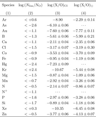
Table 3. Comparison with Meteoritic and Solar Abun-dances
Species log (Nlim/NO) log (X/O)CI log (X/O)
(1) (2) (3) (4) Ar < +0.6 −8.90 −2.29 ± 0.14 As < −2.6 −6.10 ± 0.06 · · · Au < −1.1 −7.60 ± 0.06 −7.77 ± 0.11 B < −1.3 −5.61 ± 0.06 −5.99 ± 0.21 Ca < −1.1 −2.11 ± 0.04 −2.35 ± 0.06 Cl < −1.5 −3.17 ± 0.07 −3.19 ± 0.30 Co < −0.9 −3.53 ± 0.04 −3.70 ± 0.09 Fe < −0.9 −0.95 ± 0.04 −1.19 ± 0.06 Hg < −2.4 −7.23 ± 0.09 · · · Kr < +2.4 −10.67 −5.44 ± 0.08 Mg < −1.5 −0.87 ± 0.04 −1.09 ± 0.06 Mn < −0.7 −2.92 ± 0.04 −3.26 ± 0.06 N < −0.5 −2.14 ± 0.07 −0.86 ± 0.07 N+ < −1.1 · · · · P < −1.6 −2.97 ± 0.06 −3.28 ± 0.06 Si < −1.7 −0.89 ± 0.04 −1.18 ± 0.06 Xe < +0.3 −10.35 −6.45 ± 0.08 Zn < −0.5 −3.77 ± 0.06 −4.13 ± 0.07 Note—Limits are quoted at the 99% confidence level.
The column density of oxygen for the grand sum is hNOi = 7.0 × 1011 cm−2. Abundance ratios for CI
carbonaceous chondrites and the solar photosphere are fromLodders, Palme, & Gail(2009) andAsplund et al.
(2009), respectively.
5.2. Comparisons with Meteoritic and Solar Abundances
We compare our column density limits to CI carbona-ceous chondrite (Lodders et al. 2009) and solar photo-spheric (Asplund et al. 2009) abundances inTable 3. We choose to compare to CI carbonaceous chondrite abun-dances because they are well-known and consistent with the mean elemental abundances in Stardust samples of Comet 81P/Wild 2 (Flynn et al. 2006). Note that As-plund et al. (2009) use indirect photospheric estimates for the noble gases.
To facilitate these comparisons, we normalize our col-umn density limits by the colcol-umn density of O, which we derive from the best-fit brightness to the O 1302 Å line using hgOi = 1.70 × 10⁻⁵ photons s−1. We
normal-ize by O instead of H because it is less volatile and has no contamination from the interplanetary medium (e.g.,
Vincent et al. 2014). For all but the most volatile ele-ments (e.g., N and the noble gases), the meteoritic and
photospheric abundances relative to O are comparable, and often indistinguishable within the statistical uncer-tainties.
The Alice upper limits are orders of magnitude above the expected ratios, except for Fe/O, Mg/O, and Si/O. Fe, Mg, and Si are all refractory elements common to mineral grains, and only expected to enter the coma via sputtering. Wurz et al. (2015) suggest that the amounts of Mg and Fe sputtered may be comparable to the amount of Si, but ROSINA/DFMS cannot constrain these species due to low detection efficiencies and inter-ferences. Thus, we attribute the low Fe/O, Mg/O, and Si/O limits found by Alice near perihelion to the pres-ence of the comet’s solar-wind and diamagnetic cavities.
6. SUMMARY
We have presented upper limits for 18 species in the coma of 67P/C-G, derived from a “grand sum” of expo-sures obtained by Rosetta’s Alice far-UV imaging spec-trograph near perihelion. Essential steps in our proce-dure were carefully selecting and vetting which expo-sures contribute to the coaddition, and fitting and re-moving backgrounds from reflected solar continuum and gaseous H2O vapor in the coma and ubiquitous
emis-sions from H, O, C, S, and CO. Upper limits were de-rived by direct integration of the fit residuals.
Our upper limits for the noble gases Ar and Xe were a factor of 4 and 50, respectively, larger than estimates of the bulk abundance relative to H2O derived from
ROSINA measurements (Rubin et al. 2018). On the other hand, our upper limits for Ca and Si were a factor of 2.4 and 670 below those observed by ROSINA in 2014 October (Wurz et al. 2015), offering indirect evidence that the solar-wind and diamagnetic cavities of 67P/C-G (Behar et al. 2017; Goetz et al. 2016) prevented the solar wind from sputtering dust grains on the nucleus near perihelion. Our upper limits on Fe/O and Mg/O compared to meteoritic (Lodders et al. 2009) and so-lar (Asplund et al. 2009) abundances also support this conclusion.
Rosetta is an ESA mission with contributions from its member states and NASA. We thank the members of the Rosetta Science Ground System and Mission Operations Center teams, in particular Richard Moissl and Michael Küppers, for their expert help in planning and execut-ing the Alice observations. The Alice team acknowledges support from NASA via Jet Propulsion Laboratory con-tract 1336850 to the Southwest Research Institute.
Facility:
Rosetta (Alice)Rosetta Upper Limits 9 REFERENCES
Acton, C. H. 1996, Planet. Space Sci., 44, 65
Ajello, J. M., Malone, C. P., Evans, J. S., et al. 2019, Journal of Geophysical Research (Space Physics), 124, 2954
Altwegg, K., Balsiger, H., Berthelier, J. J., et al. 2017, MNRAS, 469, S130
Asplund, M., Grevesse, N., Sauval, A. J., & Scott, P. 2009, ARA&A, 47, 481
Balsiger, H., Altwegg, K., Bochsler, P., et al. 2007, SSRv, 128, 745
Balsiger, H., Altwegg, K., Bar-Nun, A., et al. 2015, SciA, 1, e150037
Behar, E., Nilsson, H., Alho, M., Goetz, C., & Tsurutani, B. 2017, MNRAS, 469, S396
Bieler, A., Altwegg, K., Balsiger, H., et al. 2015, Nature, 526, 678
Biver, N., Hofstadter, M., Gulkis, S., et al. 2015, A&A, 583, A3
Bockelée-Morvan, D., Debout, V., Erard, S., et al. 2015, A&A, 583, A6
Bockelée-Morvan, D., Crovisier, J., Erard, S., et al. 2016, MNRAS, 462, S170
Calmonte, U., Altwegg, K., Balsiger, H., et al. 2017, MNRAS, 469, S787
Cashman, F. H., Kulkarni, V. P., Kisielius, R., Ferland, G. J., & Bogdanovich, P. 2017, ApJS, 230, 8
Conway, R. R. 1981, J. Geophys. Res., 86, 4767 Coradini, A., Capaccioni, F., Drossart, P., et al. 2007,
SSRv, 128, 529
Feldman, P. D., A’Hearn, M. F., Bertaux, J.-L., et al. 2015, A&A, 583, A8
Feldman, P. D., A’Hearn, M. F., Feaga, L. M., et al. 2016, ApJL, 825, L8
Feldman, P. D., A’Hearn, M. F., Bertaux, J.-L., et al. 2018, AJ, 155, 9
Flynn, G. J., Bleuet, P., Borg, J., et al. 2006, Science, 314, 1731
Fougere, N., Altwegg, K., Berthelier, J.-J., et al. 2016, MNRAS, 462, S156
Goetz, C., Koenders, C., Richter, I., et al. 2016, A&A, 588, A24
Gulkis, S., Frerking, M., Crovisier, J., et al. 2007, SSRv, 128, 561
Hansen, K. C., Altwegg, K., Berthelier, J.-J., et al. 2016, MNRAS, 462, S491
Hässig, M., Altwegg, K., Balsiger, H., et al. 2017, A&A, 605, A50
Hoang, M., Altwegg, K., Balsiger, H., et al. 2017, A&A, 600, A77
Keeney, B. A., Stern, S. A., A’Hearn, M. F., et al. 2017, MNRAS, 469, S158
Keeney, B. A., Stern, S. A., Feldman, P. D., et al. 2019, AJ, 157, 173
Kramida, A., Ralchenko, Y., Reader, J., & NIST ADS Team. 2018, NIST Atomic Spectra Database, v5.6, National Institute of Standards and Technology, Gaithersburg, MD, doi:10.18434/T4W30F.
https://physics.nist.gov/asd
Kurucz, R. L. 1999-2014, Robert L. Kurucz On-Line Database of Observed and Predicted Atomic Transitions, Smithsonian Astrophysical Observatory, Cambridge, MA.
https://kurucz.harvard.edu/atoms/
Läuter, M., Kramer, T., Rubin, M., & Altwegg, K. 2019, MNRAS, 483, 852
Le Roy, L., Altwegg, K., Balsiger, H., et al. 2015, A&A, 583, A1
Lodders, K., Palme, H., & Gail, H. P. 2009, Landolt Börnstein, 4B, 712
Lupu, R. E., Feldman, P. D., Weaver, H. A., & Tozzi, G.-P. 2007, ApJ, 670, 1473
Marshall, D. W., Hartogh, P., Rezac, L., et al. 2017, A&A, 603, A87
Marty, B., Altwegg, K., Balsiger, H., et al. 2017, Sci, 356, 1069
Migliorini, A., Piccioni, G., Capaccioni, F., et al. 2016, A&A, 589, A45
Noonan, J., Schindhelm, E., Parker, J. W., et al. 2016, AcAau, 125, 3
Noonan, J. W., Stern, S. A., Feldman, P. D., et al. 2018, AJ, 156, 16
Pineau, J. P., Parker, J. W., Steffl, A. J., et al. 2019, Journal of Spacecraft and Rockets, 56, arXiv:1711.02811 Rottman, G. J., Woods, T. N., & Sparn, T. P. 1993,
J. Geophys. Res., 98, 10,667
Rubin, M., Altwegg, K., Balsiger, H., et al. 2017, A&A, 601, A123
—. 2018, Science Advances, 4, eaar6297 Stern, S. A. 1999, SSRv, 90, 355
Stern, S. A., Slater, D. C., Scherrer, J., et al. 2007, SSRv, 128, 507
Swings, P. 1941, Lick Observatory Bulletin, 19, 131 van Hoof, P. A. M. 2018, Galaxies, 6, 63
Vervack, Jr., R. J., Weaver, Jr., H. A., Knight, M. M., et al. 2017, AGU Fall Meeting Abstracts
Vincent, F. E., Katushkina, O., Ben-Jaffel, L., et al. 2014, ApJ, 788, L25
Wilhelm, K., Lemaire, P., Curdt, W., et al. 1997, SoPh, 170, 75
Wurz, P., Rubin, M., Altwegg, K., et al. 2015, A&A, 583, A22