Development of models for the sodium version of the two-phase three dimensional thermal hydraulics code THERMIT

(1)

Development of Models for the Sodium Version of the Two-Phase Three Dimensional

Thermal Hydraulics Code THERMIT by

Gregory J. Wilson Mujid S. Kazimi

Energy Laboratory Report No. MIT-EL 80-010

(2)

(3)

VERSION OF THE TWO-PHASE THREE DIMENSIONAL

THERMAL HYDRAULICS CODE THERMIT

by

Gregory J. Wilson Mujid S. Kazimi

Energy Laboratory and

Department of Nuclear Engineering

Massachusetts Institute of Technology Cambridge, Massachusetts 02139

Topical Report of the MIT Sodium Boiling Project

ABSTRACT...

...

ACKNOWLEDGEMENT . . . . TABLE OF CONTENTS... List of Figures. , . . . . List of Tables . . . . Nomenclature . . . .. . . . Chapter 1: INTRODUCTION . . . .

1.1 Description of THERMIT for Sodium ....

1.2 Models Developed . . . .

1.2.1 Fluid Conduction Model . .. ..

1.2.2 Structure Conduction Model . . . . 1.2.3 Fuel Rod Conduction Model . . . . .

1.2.4 Interfacial Exchange Coefficients .

1.2.5 Friction Factor Correlations . . .

1.3 Chapter 2.1 2.2 2.3 2.4 2.5 Chapter 3.1 3.2 3.3 Results . . . .

2: FLUID CONDUCTION MODEL. . .

Basic Assumptions . . . .

Fully Explicit Formulation . .

Partially Implicit Formulation

Programming Information . .

Sample Cases . . . .

3: STRUCTURE CONDUCTION MODEL.

Basic Assumptions . . . . Boundary Conditions . . . . . Method of Solution . . . . 1 2 3 4 7 11 14 14 18 18 18 19 21 22 . . . 23 . . . 25 . . . 25 . . . 26 . . . 32 . . . 33 . . . 34 . . . 40 . . . 40 . . . 43 . . . 47

(14)

-5-Page

3.4 Programming Information . . . 52

3.5 Sample Cases . . . 56

Chapter 4: FUEL ROD CONDUCTION MODEL . . . 63

4.1 Features of Model . . . 63

Chapter 5: INTERFACIAL EXCHANGE COEFFICIENTS . .· 73

5.1 Mass Exchange Coefficient .. . . . 73

5.2 Momentum Exchange Coefficient . . . 84

Chapter 6: FRICTION FACTOR CORRELATIONS . .. . . 95

6.1 Axial Friction Factor - Single Phase Liquid . . . 95

6.2 Axial Fiction Factor - Two Phase Flow . 108 6.3 Transverse Friction Factor . . . 113

Chapter 7: VERIFICATION OF MODELS AND APPLICATION TO LMFBR CONDITIONS . . . . 119

7.1 Purpose

.

. . . .119

7.2 Description of the THORS Bundle 6A Experiments . . . 120

7.3 THERMIT Simulation of THORS Bundle 6A, Test 71h, Run 101 . . . 124

7.4 LMFBR Fuel Assembly Simulation ... . 139

Chapter 8: SUMMARY AND RECOMMENDATIONS . . . 147

8.1l Models and Correlations . . 147

8.2 General . . . 150

(15)

Page

Appendix A: THERMIT FOR SODIUM - INPUT

DESCRIPTION . . . 155

Appendix B: INPUT FILES FOR THERMIT TEST CASES . . 166

B.1 4 Channel Steady State Conduction

Test Case . . . 166

B.2 9 Channel Transient Conduction

Test Case (Explicit) . . . 167

B.3 9 Channel Transient Conduction

Test Case (Semi-implicit) . . . 168

B.4 THORS Bundle 6A Simulation, Case A

(No Heat Losses, No Plenum) . . . 169

B.5 THORS Bundle 6A Simulation, Case B

(Heat Losses to Sodium-soaked Insulation,

No Plenum) . . . 171

B.6 THORS Bundle 6A Simulation, Case C

(Heat Losses to Sodium-soaked Insulation,

Gas Plenum Conduction) . . . 172

B.7 217 Pin Bundle Simulation, Case D

(No Heat Losses, No Plenum) . . . ... 173

B.8 217 Pin Bundle Simulation, Case E

(Heat Losses to Hex Can, No Plenum) . . .. 174

B.9 217 Pin Bundle Simulation, Case F (Heat Losses to Hex Can + Insulation,

(16)

-7-LIST OF FIGURES

Number Page

2.1 Top View of Fluid Channels . . . 28

2.2 Closeup of Two Fluid Channels, Showing the Heat Transfer Between Them. .30

2.3 Fluid Conduction Test Case - 4 Channel ... . 35

2.4 Geometry for 9 Channel Fluid Conduction Test

Case (Top View) . . . 37

2.5 Fluid Conduction Test Case - 9 Channel

(Explicit Run) . . . 38

2.6 Fluid Conduction Test Case - 9 Channel

(Semi-implicit Run) . . . 39

3.1 Hex Can with Associated Structure . . . 42

3.2 THERMIT Model of Hex Can with Associated

Structure ... ... . 44

3.3 Mesh Cell Representation of Structure . . . 48

3.4 Temperature Distribution of Cylinder Initially at 500°k, Placed in a 200°k

Environment . . . 57

3.5 Centerline Temperature of Cylinder vs.

Theoretical Prediction . . . . 58

3.6 Surface Temperature of Cylinder vs.

Theoretical Prediction . . . 59

3.7 Temperature Distribution of Two-component Annulus Initially at 500°k, Subjected to Different Boundary Conditions at the Inner

and Outer Surfaces . . . 61

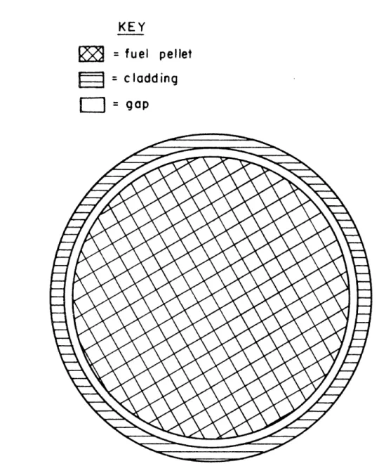
4.1 Three Zone Fuel Rod (Top View). 64

4.2 Five Zone Fuel Rod (Top View) . . . 65

4.3 Fuel Rod with Gas Plenum (Side View). . . . 67

(17)

List of Figures (continued)

Number

5.2 Annular Flow in Triangular Rod Arrays . .

5.3 Interfacial Area of Mass Exchange

vs. a (D=0.25") . . . .

5.4 Interfacial Area of Mass Exchange

vs. a (D=0.50") . . . .

5.5 Values of Pe and K for a Transient in a

eTypical

LMFBR

Typical LMFBR . ...

5.6 Values of re and K at Steady State in a

eTypical LMBR

Typical LMFBR ...

6.1 Different Types of Subchannels in a

19 Pin Bundle . . . .

6.2 Axial Friction Factor vs. Re for a 61 Pin

Blanket Assembly . . . ..

6.3 Axial Friction Factor vs. Re for a 217 Pin

Fuel

Assembly

_....

_...

6.4 THERMIT Axial Friction Factors vs. Re for

61 and 217 Pin Assemblies . . . .

7.1 Cross Section of THORS Bundle 6A . . . . .

7.2 THORS Bundle 6A Fuel Pin Simulator . ...

7.3 Temperature and Pressure vs. Time for

Test 71h, Run 101 . . . .

7.4 Mesh Spacing Used in THERMIT Simulations of

THORS Bundle 6A Experiments . . . .

7.5 THORS Bundle 6A - Axial Temperature Distri-bution at Start of Transient (Test 71h, Run

7.6 THORS Bundle 6A - Temperature History

at z=30 inches (Test 71h, Run 101) . . . .

7.7 THORS Bundle 6A - Temperature History

at z=34 inches (Test 71h, Run 101) . . . .

Page 80 82 83 90 -~. 91 . . . 100 . . . 104 . 105 . 109

*

.

122

*

.

123 . . 125 . . 128 101) 131 . 133 . . 134

(18)

-9-List of Figures (continued)

Number Page

7.8 THO)RS Bundle 6A - Temperature History

at z=54 inches (Test 71h, Run 101). 135 7.9 217 Pin Bundle - Temperature History

at z=?2 inches . . . ... 142

7.10 217 Pin Bundle - Temperature History

at z=30 inches . .. . . 143

7.11 217 Pin Bundle - Temperature History

(19)

Number Page

5.1 Parameters Used in Comparison of K vs. r . . . 92 e

6.1 Range of Data for Various Axial Friction

Factor Correlations ... . 98

7.1 Boiling Inception Times for THORS Bundle 6A

Simulations . . . 137

7.2 Boiling Inception Times for 217 Pin Bundle

(20)

-11-NOMENCLATURE Letter A A cf C p D De Dh D V

_v

f F g G h

hin

_in

Definition Units (SI)

Flow area

Interfacial area of mass exchange Contact fraction Specific heat Diameter Equivalent diameter Hydraulic diameter Volumetrically defined hydraulic diameter Friction factor

terfacial

H k K L N Nu p P

Pe

Pe Pr q q" qlll

Force per unit volume

Gravitational acceleration Mass flux

Heat transfer coefficient Two-fluid heat exchange

coefficient

Wire wrap lead length Thermal conductivity

Momentum exchange coefficient Length Bubble density Nusselt number Pressure Pitch Heated perimeter Peclet number Prandtl number Heat flow Heat flux Heat generation 2 rn m

_-1

m J/kg°K m m m Tn N/m3 2

m/sec2

kg/m2sec W/m2OK W/m3OK m W/m°K kg/m3sec

m

-3 N/m2 m m W W/m2 W/m3

(21)

Nomenclature (continued)

Definition Units (SI)

Radius

Reynolds number

Gas constant for sodium Time Temperature Velocity Velocity Volume Quality

Flow split parameter

Two phase Martinelli parameter Spatial coordinates

Thermal diffusivity Void fraction

Mass exchange coefficient Constant in interfacial mass

exchange coefficient Viscosity

Density

Two phase friction multiplier

2 m /sec 3 kg/m3sec kg/m sec kg/m3 N Superscripts

Old time level New time level

Subscripts Bubble Letter r Re R g t T u

v

V V x X

Xtt

x,y, z m J/kg°K sec oK m/sec m/sec 3 m m Greek a a P X V1 P n n+l b

(22)

-13-Nomenclature (continued) Subscripts Definition c Condensation e Evaporation i Interface i Node number P Liquid

N Total number of nodes

s Saturation

T Total

TP Two phase

v

Vapor

(23)

Chapter 1: INTRODUCTION

1.1 Description of THERMIT for Sodium

The computer code THERMIT was developed at MIT in

order to model transient situations in light water reactor

cores. The work described in this thesis was part of a

project undertaken at MIT to modify THERMIT to be able

to analyze sodium-cooled reactor cores. For the sake of

clarity, it is necessary to provide a brief description

of the code before describing the modifications made to it.

This section will describe the characteristics, solution

technique, and some of the restrictions of THERMIT. For

more details the reader should refer to Reference [1].

Several people have been involved in the adaptation of

THERMIT to sodium. This section will review their work,

also. The next section will introduce the models I have

developed, which constitute the bulk of this thesis.

THERMIT is a three dimensional transient, two phase,

thermal-hydraulics code that simulates conditions in a

reactor core. It uses a rectangular (x,y,z) coordinate

system. Only the thermal-hydraulic aspects of the reactor

are considered (neutronic effects are ignored). This

(24)

-15-space and time. THERMIT uses the two-fluid model for two

phase (i.e. vapor and liquid) flow. This models the

liquid and vapor as separate fluids coupled by exchange

coefficients. Thus, six fluid dynamics equations must be

solved (conservation of mass, momentum, and energy for

both phases). In order to simulate a transient, THERMIT

is run until a steady state is achieved, and then the

necessary parameters are altered, producing the transient

results. In addition to the fluid dynamics calculations,

THERMIT solves the radial heat conduction problem in the

fuel rods (neglecting axial and azimuthal conduction).

The method of solution of the fluid dynamics equations

is what distinguishes THERMIT most from other fluid

dynamics codes. THERMIT uses a partially implicit scheme

in solving the first order finite difference form of the

equations. The terms involving sonic velocity and

inter-facial exchange have been treated implicitly. Only the

liquid and vapor convection terms are treated explicitly,

and this introduces a time step limitation. The equations

are solved by a two-level iteration procedure. Each time

step advancement is reduced to a Newton iteration problem.

Each Newton iteration is in turn reduced to a set of linear

equations in pressure alone, which is solved by a block

(25)

equations are solved implicitly, and are coupled to the

fluid with a fully implicit boundary condition (see

Appendix E of Ref. [1]).

THERMIT does have some restrictions, other than the

time step limit just mentioned. The partial differential

equations are not well-posed in the mathematical sense.

This means that the size of the fluid mesh cells cannot

be exceedingly small, or the solution will not be

well-behaved.

THERMIT allows considerable flexibility in the

bound-ary conditions at the inlet and the outlet. The user may

specify either pressure or velocity boundary conditions.

In the case of a transient these values may vary with time

according to a user-supplied table. The capability of

varying power with time exists also.

Many changes were made in the water version of THERMIT

in order to convert it to sodium. The remainder of this

section will briefly describe the changes made by M.

Manahan, A. Schor, R. Vilim, and A. Cheng (see Reference

[18]).

As previously mentioned, THERMIT uses rectangular

coordinates. In analyzing LWR square array rod bundles

only one axial hydraulic diameter was required as user

(26)

-17-necessitated the modification of THERMIT to accept radially

variable heated and wetted equivalent diameters.

The bulk of the work done on THERMIT involved

replac-ing all the equations and correlations developed for water

with the appropriate ones pertaining to sodium.

Correla-tions for the following physical properties were employed:

saturation temperature, surface tension, and liquid and

vapor internal energies, densities, conductivities, and

viscosities. A new correlation for the heat transfer

coefficient at the fuel-sodium interface was developed and

implemented.

Work is currently underway to implement an improved

model for calculating the geometry and material properties

of the fuel rod. This model will be more applicable to an

LMFBR fuel rod than the previous one. It will be able to

handle such phenomena as restructuring of fuel and dynamic

gap conductance.

The final changes to be described in this section were

designed to accelerate convergence. First of all, the code

was converted to double precision. This reduced the

round-off error. The second change was to allow the suppression

of transverse velocities. This significantly reduced the

time necessary to reach a steady state, and therefore

(27)

1.2- Models Developed

1.2.1 - Fluid Conduction Model

In the water version of THERMIT the only mechanism by

which heat may be transferred between two adjacent fluid

mesh cells is through transverse velocities. Thus, if the

transverse velocities are low, the rate of heat transfer

is low also. Clearly there will be heat transfer between

cells due to conduction, even if the transverse velocities

are zero. In the case of water, which does not have an

exceptionally high thermal conductivity, the loss of

accu-racy may not be that great, but for liquid sodium,where

the thermal conductivity is two orders of magnitude greater

than water, conduction effects cannot be ignored.

Therefore, a radial heat conduction capability has

been incorporated in THERMIT for sodiuwn. This model is

described in detail in Chapter 2. The model only applies

in the single phase liquid region, because upon boiling

the thermal conductivity of sodium drops so drastically

as to make conduction effects negligible. Axial

conduc-tion is not included, because convecconduc-tion is far more

important, except in cases of extremely low flow.

1.2.2 - Structure Conduction Model

In the water version of THERMIT the outer boundary of

(28)

-19-to be adiabatic. In other words, no heat is allowed to

leave the system in the radial direction. When modeling

large systems (for example, an entire reactor core) this

is not a bad assumption, but for smaller systems (like a

single rod bundle) radial heat losses to the structure

surrounding the system may be significant. Once again,

the effect is more pronounced with liquid sodium than

with water, due to the large thermal conductivity of the

former. As with the fluid conduction model, no heat is

lost from fluid cells in which vapor is present.

Chapter 3 describes the structure conduction model

in detail. The model employed is similar in many respects

to the fuel rod conduction model in the water version of

THERMIT. The structure is represented by a user-specified

number of concentric radial regions, each of which may

contain a different material. Therefore, composite

structures may be represented. All calculations (except

the coupling term with the fluid dynamics) are performed

implicitly. This model may be bypassed, if so desired,

thus simulating the adiabatic condition previously in

THERMIT.

1.2.3 - Fuel Rod Conduction Model

A new and much more general fuel rod model has been

(29)

previous version allowed only three radial zones in the

fuel rod (representing the fuel, clad, and gap). This

model is inadequate for representing such phenomena as

fuel redistribution and central voiding. The new fuel

rod conduction model (described in detail in Chapter 4)

permits the user to specify the number of radial zones

desired and the thermal properties of each. The second

major modifidation is that the structure of the fuel rod

may be varied axially as well. The water version of

THERMIT required the structure of the fuel rod to remain

constant in the axial direction. In order to model the

gas plenum region of the LMFBR fuel rod, axially variable

fuel rod properties must be permitted. This is done

by allowing the user to specify the number of axial

regions desired and the geometry and materials in each

region.

The solution scheme for the fuel rod conduction has

not been altered. Only the arrays containing the

geomet-rical parameters and thermal properties were changed.

This involved altering many input parameters. These

changes are described in detail in Section 4.2 and are

summarized in the input description of THERMIT for sodium

(30)

-21-1.2.4 - Interfacial Exchange Coefficients

The most uncertain aspect of the two fluid equations

is the form of the interfacial exchange coefficients,

which represent the mass, momentum and energy transfer

between the liquid and vapor phases. The values of these

coefficients are very uncertain even for water, but for

sodium this is even more true.

Chapter 5 describes the correlations adopted for the

mass and momentum exchange coefficients in the sodium

version of THERMIT. In the case of the energy exchange

coefficient a large constant (hinterfacial = 1.0 1010

W/m3 °K) is assumed. This forces near thermal equilibrium

between phases.

For the mass exchange coefficient a modified version

of the Nigmatulin Model [7] is used. The original model

assumes bubbly flow, with a constant bubble density. In

sodium boiling at low pressures the annular flow regime

dominates, for large void fractions. The revised model

takes this into account in developing a mass exchange

coefficient that is dependent on the flow regime

encoun-tered.

The momentum exchange coefficient is taken from

M.A. Autruffe [9]. This correlation was derived from

single tube sodium boiling data. In addition, the

(31)

included. This effect was neglected in the water version

of THERMIT. Section 5.2 shows that at large void

frac-tions this phenomena can be important, however.

It should be noted that these correlations have

not been tested very extensively, especially in

trian-gular rod bundle geometries, so their applicability is

not beyond question. They do represent the best

informa-tion available, however. The modular construcinforma-tion of

THERMIT permits the user to incorporate new correlations

quite easily, as they become available.

1.2.5 - Friction Factor Correlations

In the two-fluid formulation of two phase, three

dimensional flow it is necessary to supply liquid and

vapor friction factors for both the axial and the

trans-verse directions. Because of the complex geometry

involved in LMFBR reactor cores, no one correlation can

be applied directly for either direction. Chapter 6

describes the combinations of correlations incorporated

in the sodium version of THERMIT.

For the liquid friction factor in the axial

direc-tion, the flow is divided into three categories: laminar

(Re'< 400), turbulent (Re > 2,600), and transition (400 < Re < 2,600). Separate correlations are used for

lam-inar and turbulent flow, while a combination of the two

(32)

-23-The vapor friction factor in the axial direction is

much less refined, due to lack of data. A turbulent

formula developed for flow in a pipe is employed over

the full Reynolds Number range. Because the sodium

version of THERMIT assumes dryout occurs for void

frac-tions above 0.957, the vapor does not come in contact

with the fuel rod below this value. Therefore, the vapor

friction factor is zero in this range.

The friction factors in the transverse direction are

basically the same as those described in the THERMIT

des-cription (Reference 13), with the exception that because

of the assumption that no vapor comes in contact with the

wall for void fractions below 0.957 the vapor friction

factor is zero in this region. Some modifications have

also been made in the form of the laminar friction factors

in two phase flow. See Section 63 for details.

1.3 Results

Chapter 7 discusses the results obtained from six runs

made with THERMIT. Cases A, B, and C were simulations

of the THORS Bundle 6A experiments done at Oak Ridge [6].

These simulations show the value of the structure

conduc-tion and fuel rod models in improving the predicconduc-tions of

THERMIT for this 19 pin bundle. Cases D, E, and F extend

(33)

River Breeder Reactor. These final three cases evaluate

the relative importance of the inclusion of radial heat

losses when modeling loss-of-flow transients in LMFBR's.

Finally, Chapter 8 summarizes the findings of this

thesis, and makes recommendations for future work in

improving the capability of THERMIT to model transients

(34)

(35)

Chapter 2: FLUID CONDUCTION MODEL

2.1 Basic Assumptions

Two options have been developed in THERMIT for the

inclusion of heat conduction between adjacent fluid

chan-nels. The first option is a fully explicit formulation,

while the second is partially implicit, and will be

des-cribed in Section 2.3. Both models contain certain basic

assumptions.

The first assumption made is that the conduction

effects become negligible when boiling occurs in at least

one of the two adjacent channels. This is justified under

normal reactor conditions, because the thermal conductivity

of sodium vapor is significantly less than that of liquid

sodium (i.e. at 800°k, k = 66.98 W/m'k and kv =5.42 x

1-2W/o

10 W/mk, so k/kv 1236). This radical change in thermal

conductivity, coupled with the extremely high void fractions

encountered in sodium boiling at low pressures, ensures that

liquid-to-vapor and vapor-to-vapor conduction effects are

completely negligible. Therefore, when boiling occurs in

a channel conduction heat transfer through its faces is

neglected.

Only radial conduction is incorporated in THERMIT

now, although the model permits the inclusion of axial

(36)

-26-dominates the heat transfer, due to the large axial velocity

of the liquid sodium. Only in cases of extremely low flow

will axial conduction become significant. For example,

it has been shown that for the Clinch River Breeder Reactor

core the velocity could be reduced by at least three orders

of magnitude before axial conduction effects become as

large as 2% (Reference 2]).

The third major assumption is that the effective

Nusselt Number for conduction (defined below) is a constant,

independent of fluid conditions. This assumption is

neces-sitated by the lack of data available for sodium flow in

the geometry modeled in THERMIT. The current fluid

con-duction model allows the user to input a value for the

Nusselt Number, which remains constant throughout the

cal-culation. If in the future a Nusselt Number correlation

is developed for this type of geometry it could be

incor-porated with a minimum amount of work.

It should be noted that this model only considers

heat transfer between fluid channels. The heat flow through

all external faces is taken into account in the model

des-cribed in Chapter 3.

2.2 Fully Explicit Formulation

The net rate of flow of heat into a given fluid cell

is expressed as the sum of the heat fluxes from each of

(37)

4m00-the four sides (ignoring 4m00-the two sides perpendicular to

the axial direction). The heat flow term for each side

is calculated by multiplying the temperature difference

by an effective conduction heat transfer coefficient.

For the configuration of Figure 2.1,

(n+l) = A - T (n) (), and (2-1)

qlO

A-0h10(

'

TLO

n

21

q(n+l) =q(n+l) + q(n+l) + (n+l) + q(n+l) (2-2)

2-0 q₃-₀ 4-0

where

ql-O = heat flow from channel 1 to channel 0 (W),

qT = total heat flow into channel 0 (W),

A₁ ₀ = heat flow area between channels 1 and 0 (m2),

hl ₀ = effective conduction heat transfer coefficient

2

between channels 1 and 0 (W/m 2°k),

T, and Ti are the liquid temperatures in channels

0 and 1, respectively. The superscripts refer to the time

step at which the quantities are measured. Note that in n+l

Equation (2-1) the heat flow, ql-,' is calculated entirely

from quantities evaluated at time step n. This is what makes

the method explicit.

Referring to Equation (2-1), the quantity A ₀ is known

from geometry, and Ttn) and T(n) are known from the solution

of the problem at time step n, so only h(n) remains to be 1-0calculated. This is done by considering the problem as calculated. This is done by considering the problem as

(38)

-28-Top View of Fluid Channels

(39)

two resistances in series (see Figure 2.2). An interface

temperature, T_i, is defined at the boundary between the

two channels, and the heat transfer coefficients within

each channel, h1 and h0, are defined as:

q'- = h(T

i

- T

0

) = h(T,

-

T

(2-3)

To calculate h₀ and h₁ the constant Nusselt Number

approximation described above is used:

k k

h _{= NDe}= Nu- , h1 =Nu , (2-4)

0 = De 1

where

k = thermal conductivity of sodium (W/m°k), 4 x Af

De = equivalent diameter = P (m), Ph = heated perimeter of channel (m),

h~~~~~~~~~~~~~~~

Af = cross-sectional flow area of channel (m )

Solving Equation (2-3) for Ti,

T. = T~ 1 + h 0TZ 0

T. h+ h (2-5)

i h1 0

Rearranging Equation (2-1), and substituting Equation

(2-3),

~h

qq

l' h₀(T_i - T,₀

)

1-0hT

=

-

-T

(2-6)

(40)

-30-Figure 2.2

C

T

Tt, 0

I

l

i

I~k I I I I "I I 1 4

loseup of Two Fluid Channels, Showing the Heat Iransfer Between Them

II

jql_ 0

i

(41)

Finally, introducing Equation (2-5) into (2-6),

hlh₀

hl_ h + h 0 (2-7)

Therefore, the solution technique for the fully

ex-plicit model is as follows: given the geometry of the

problem, solve Equations (2-4) for h and h, use Equation

(2-7) to obtain h ₀, and plug the results into (2-1) to

get q(n+l) _ge_q-0' These steps are repeated for each face of the channel.

The major advantage of the explicit method is that it

uses very little computer time, and is therefore inexpensive.

In addition, it ensures strict conservation of energy (i.e.

q(n+l) = q(n+l))* The disadvantage of the explicit method ql-0 = 0-1'

is that it introduces a stability limit on the time step

size that may be more restrictive than the convective limit

currently used in the code. The time step limitation for

conduction in two dimensions [3] is:

At < a (2-8)

4ct

where = thermal diffusivity = k . PCp

When using a very fine mesh the explicit method can

introduce unreasonable limitations on the time step size.

In most cases, however, the convective limit will be more

(42)

-32-2.3 Partially Implicit Formulation

The partially implicit formulation currently in

THERMIT was developed at M.I.T. by Andrei Schor for the

purpose of circumventing the stability problem introduced

by the explicit model. Equations (2-1) and (2-2) are

modified so as to be implicit in one temperature:

q(n+l) A h(n) (n) - T(n+l)) (2-9) 1-0 (T1,i ,0 q(n+l) A h(n) (T (n) T(n+l)) + A h(n)(T(n) _ T(n+l)) T -01-0 -' O,1 Q 2-0 2-0 h,2 ( n + A h(n)(T(n) _ T(n+l)) + A h(n) (T(n) _ T(n+l) (2-10) 3 -0 ,3 Zt ( 4-0 40 , 0

This formulation avoids the time step limitation of the

explicit method, but it introduces another problem: lack

of energy conservation. The heat flow from channel 1 to

channel 0, q ₀, should have the same magnitude (but opposite

sign) as the heat flow from channel 0 to channel 1, q0-1

This is certainly the case in the explicit formulation, where

both T ₀ and T ₁ are evaluated at the old time step, but in the partially implicit method this condition is only

satis-fied if T(n) - T(n+O)=T(nl) - T n) which is not true in

9~,0 -=li,l 0

general .

Thus the choice between the fully explicit and partially

implicit formulations involves a trade-off. The explicit

(43)

limitation on the time step size, while the partially

implicit method avoids the time step limitation, but fails

to strictly conserve energy.

2.4 Programming Information

This section is designed to supplement the THERMIT

Users' Manual [1], in explaining the implementation of the

models discussed in the previous two sections.

The fluid conduction model requires only one additional

input variable above those described in Reference [1] (see

Appendix A for the complete input description for the sodium

version of THERMIT). The user specifies the conduction

Nusselt Number, "rnuss", which is used in Equation (2-4).

If a positive real number is entered, the partially implicit

method is used, with Nu = "rnuss", while a negative real

number specifies the explicit option, with Nu = -"rnuss".

(The number 7.0 is recommended for "rnuss"I, because it represents a typical value for the Nusselt Number in liquid

sodium.) A value of 0.0 allows the user to bypass the

con-duction model completely.

The inclusion of the fluid conduction model required

the addition of two subroutines to THERMIT. The first one,

QCOND, is called from subroutine NEWTON, and performs the

bulk of the calculations. It calls another new subroutine,

HTRAN, which solves Equations (2-4) and (2-7). The result

(44)

-34-flow into each fluid cell (see Equation (2-2)). This array

is passed into subroutine JACOB, which solves the mass and

energy equations. If the partially implicit option is

chosen, an additional derivative term is included in the

Jacobian matrix.

2.5 Sample Cases

The explicit version of the fluid conduction model in

THERMIT has been tested for two cases. The first was a

four channel (2x2) steady-state run in which two diagonally

opposite channels were heated by fuel pins, while the other

two were unheated. All transverse velocities were set equal

to zero. This insured that any heat transfer between adjacent

channels was due to conduction alone. Temperatures were

cal-culated at sixteen axial positions, of which only the second,

third and fourth were heated. Appendix B.1 contains the

THERMIT input file for this run.

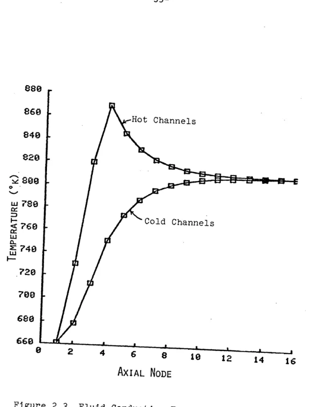
The results of the simulation are shown in Figure 2.3.

The heated channels increased in temperature up to the top

of the heated section (node four), and then cooled off as

they lost heat to the cooler, unheated channels. The

temp-erature in the unheated channels increased steadily as they

received heat from the heated channels, until the temperatures

became nearly equal at the top of the channels.

The second test case was of an entirely different nature

(45)

ota 86(

848

82e 011

_{v ale}

I-w

680

< 60

o-_O:

I

_~~x:

₇₄₀

W

700 ¢80

660

_ - u 10 12 14 AXIAL NODE

Figure 2.3 _Fluid _Conduction

Test Case _- _{4 Channel} 16

(46)

-36-which the axial and transverse velocities were initially

set at zero, with the latter being held constant at zero

throughout the transient, for the reason described above.

The fluid was unheated, but a temperature variation between

channels was introduced (see Figure 2.4). Slight axial

velocities were induced, due to the thermal expansion and

contraction in each channel. Because of these small axial

velocities some heat was carried out of the system, so the

final equilibrium temperature was about 832.91°k, instead

of the predicted 833.33°k. The temperature vs. time history

is plotted in Figure 2.5 for the center, corner, and side

channels. A time step of 5.0 seconds was used (significantly

below the 35 second conduction limit imposed by Equation (2-8)).

As shown, all channels approached a single equilibrium

temp-erature as time progressed.

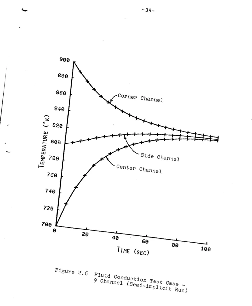
In order to test the partially implicit fluid conduction

model in THERMIT the nine channel case described above was

run again, using the same time step size (see Appendix B.3).

The results are shown in Figure 2.6. In this case the final

equilibrium temperature was only 828.65°k, 4.26 degrees less

than the final temperature of the explicit case. This

dif-ference can be attributed to the lack of strict conservation

of energy discussed in Section 2.3. As larger time steps

become necessary, however, the desirability of the partially

(47)

0.3m

E

0

!

(Numbers indicate initial temperatures in channels in °K)

Figure 2.4

Geometry for 9 Channel

Test Case (Top View)

Fluid Conduction

900

800

900

800

700

800

900

800

900 L

I i I I i I

(48)

-38-Channel Side Channel Center Channel

20

49

60

80

10

TIME (SEC)

Figure 2.5 Fluid Conduction Test Case -9 Channel (Explicit Run) 900

880

860 1% 0 -( GO

740

720 0

(49)

ee0 Corner Channel LU 0: LU LU TIME _(SEc)

Figure

_2.6

_ludCn

_pTest

Case_

9 Channel (Semi-Iie _t

(50)

(51)

Chapter 3: STRUCTURE CONDUCTION MODEL

3.1 Basic Assumptions

The structure conduction model now in THERMIT permits

the user the option of taking into account the heat losses

to the structure surrounding the region of interest. In

the previous version of THERMIT an adiabatic boundary

con-dition was assumed around the outer boundary of the region

modeled. This option still exists, if so desired. The heat

flow to the structure is calculated using a multi-layer

conduction model. Several simplifying assumptions were

necessary in order to implement the model.

The major assumption made is that of azimuthal

sym-metry. This assumption was made for two reasons. First,

in most cases there will not be much of a temperature

variation around the outside of the region modeled. Second,

far more computer storage space would be required if the

code were to calculate azimuthal temperature variations.

Therefore, only radial conduction is considered. The

structure is broken up axially into sections which coincide

with the axial fluid cells. Thus, the fluid cells at each

axial level transfer heat only to the section of the structure

that corresponds to that region. Axial conduction within the

structure is neglected also.

As in the fluid conduction model described in Chapter 2,

the heat transfer from any fluid channel in which boiling

(52)

-41-the dramatic drop in -41-the -41-thermal conductivity of sodium

upon boiling reduces the heat transfer capability so much

as to make it negligible. If some of the fluid channels

touching the structure boil, those that remain in the single

phase liquid regime continue to transfer heat to the structure.

The geometrical layout of the structure is specified

by the user, with certain restrictions. Different materials

may be used, but they must be in concentric rings around

the inner region. For example, the user could construct a

three region structure consisting of an annulus of stainless

steel surrounded by rings of insulation and stainless steel

again. The user also specifies the number of meshes desired

within each region. The temperatures are calculated at the

boundary of each mesh cell.

Only the fluid cells in physical contact with the

structure are affected by the structure conduction model.

Consider the example shown in Figure 3.1, which consists

of a single assembly encased in a hex can and surrounded

by a layer of insulation and another layer of stainless

steel. Twelve of the sixteen fluid channels touch the

structure through some portion of their perimter. These

twelve may all lose heat directly to the structure. The

four interior channels do not communicate directly with the

structure, but they do communicate with the exterior

chan-nels through the fluid conduction model described in Chapter 2.

Thus, heat generated in the interior of the region has a

(53)

stainless

steel wall

Figure 3. Hex Can with Associated Structure hpx cnn

(54)

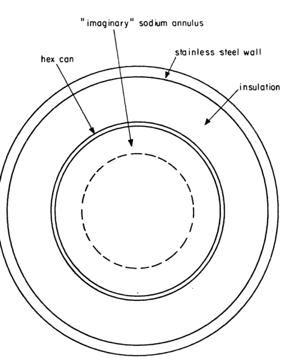
-43-A close look at Figure 3.1 will reveal that some

simpli-fications have to be made in order to represent this case

using the structure conduction model in THERMIT. The hex

can must be formed into an annulus, so as to maintain the

azimuthal symmetry required. Figure 3.2 shows this case

as it would be modeled on THERMIT. The inner boundary of

the hex can is determined by summing up the perimeters of

contact for all the exterior cells. The sodium in the

fluid channels adjacent to the structure is combined and

formed into an imaginary annulus inside the structure wall

for the purposes of calculation. The inner radius of the

sodium annulus is determined by setting the cross-sectional

area of the annulus equal to the sum of the cross-sectional

areas of the sodium in each of the fluid cells adjacent to

the structure. This averaging scheme is necessary in order

to preserve the azimuthal symmetry and to produce a geometry

for which the heat transfer characteristics are known. More

details will be given in the next section.

3.2 Boundary Conditions

In order to solve the conduction equation for the

temp-erature distribution in the structure the conditions at the

inner and outer boundaries are needed. These are provided

(55)

"imaginary" sodium annulus

stainless steel wall

Figure 3.2

Thermit Model of

Structure

(56)

-45-For the outer boundary of the structure the user

specifies a constant heat transfer coefficient and a

con-stant temperature outside the structure. Thus, the heat

flux on the outer boundary will be:

I,

t hout(T out Twall,out (3-1)

where Twall,out = the temperature at the outer boundary of

the structure. If an adiabatic condition at the outer wall

is desired, the user should set hou = 0 0. out

The boundary conditions at the inner surface of the

structure are more complicated, however, because they

in-volve heat transfer between the flowing liquid sodium and

the stationary structure. As previously mentioned, the

conditions of the sodium in each of the fluid channels in

contact with the structure must be averaged, so as to

main-tain azimuthal symmetry. Therefore, a single temperature

and pressure are calculated by taking the volume average

of these quantities in each of the separate fluid channels

in question.

Now that this "imaginary" annulus has been formed and

its properties are known the problem is to obtain a heat

transfer coefficient for the sodium/wall interface. Obviously,

no correlation exists for the actual geometry encountered,

(57)

annulus described in the previous section. O.E. Dwyer [4]

developed a Nusselt Number correlation for liquid sodium

flowing in an annulus, transferring heat through its outer

boundary: Nu hDe = A + C(iPe), (3-2) k' where A = 5.54 + 0.023(r₂/r1) C = 0.0189 + 0.00316(r₂/r₁) + 0.0000867(r₂/rl) = 0.758(r₂/r1) 00204

r = outer radius of annulus2 r = inner radius of annulus

is assumed to be 1.0. GDec

Pe = Re-Pr = P

k

Given the temperature and pressure of the sodium and

the dimensions of the annulus, k, cp, De, and G are known,

so the heat transfer coefficient, h, can be calculated.

The net heat flux on the inner boundary of the structure is

then:

q'n=

hin

(Tsodium

-

Twall

in

)

(3-3)

where Twall,in = the temperature at the inner boundary of

the structure, and hin is calculated from Equation (3-2).

This completes the list of boundary conditions necessary

(58)

-47-3.3 Method of Solution

The general equation of heat conduction is [3]:

V(kVT) + q = p t (3-4)

The situation modeled in THERMIT is considerably simpler,

though, because of the assumptions of negligible axial and

azimuthal conduction, and zero heat generation within the

structure. With these simplifications Equation (3-4) reduces

to:

3T 1 T

Pcat r ar(rka) (3-5)

cp~pr

ar

~

This equation, coupled with the boundary conditions (3-1)

and (3-3), constitutes the analytical solution to the problem.

The finite difference scheme used to solve these

equa-tions on the computer is similar to that described in Ref. [1

for the fuel rod model, with some modifications. The structure

is divided into a series of concentric rings (see Figure 3.3),

each of which shall be called a mesh cell. The properties

p, cP, and k are evaluated at the centers of the mesh cells,

while the temperatures of the structure are calculated at

the boundaries of the mesh cells (called the nodes). Both

sides of Equation (3-5) are multiplied by rdr and integrated

between the centers of the two mesh cells around node i to

(59)

mesh cell

N

Mesh Cell Representation of Structure

(60)

-49-r i+

ri+

½

J

pcpt rdr - I d(rk) = (3-6)

ri r

i-2

For the average cell, te numerical integration of

(3-6) yields:

T(n+l) _ T(n)

-T -1 (rk) i+½ (T (n+l) (n+l))

(pCp)i) i At ) (Ar) i+(i+l T

+

₊

()½(T

_(r)i(Ti

n+l)

-

T

_{i1 )}

_i

(n+l) Q

(3-7)

_(3-7)

where

2 2 2 2

__ ri+ - r_i r. - r _

(p~p _(P~Cpi½ ₂ ₌-(c)+ _(PC_/ ₌ ₊ 2 _(pcp)i-pi- _(3-8)

The superscripts refer to the time step at which the variables

are evaluated, and the subscripts refer to the mesh cell

posi-tions at which the properties are taken. Integral values

de-note nodes, while half integral values dede-note mesh cell centers.

There are two locations at which Equation (3-7) is not

valid. These are the inner surface of the structure (the

first half-cell), and the outer surface of the structure

(the last half-cell). For the inner surface of the structure

Equation (3-6) is integrated from r to r_{3 /2} This gives:

2 2

T(n+l)

_ T(n)

3/2 (p c

(PCp)

(n)1

32 (

1 -

)

r

(n+l)

k

-

T(n+l)

2 p 3/2 At - 3/2 2 1

+

rq':

=0

(3-9)

in

where qin is given by Equation (3-3). in

(61)

The outer half-cell is integrated from rN½ to rN to obtain: 2 2 T(n+l) (n) rN rN-½ (n) N TN rk) (n+l) (n+l) 2 (PCp N- At + ()N-(TN Ar) -N-1

+

rNqou

t

=0

(3-10)

where qout is given by Equation (3-1), and N = the total

number of nodes.

One further item has to be specified before Equations

(3-9) and (3-10) can be considered complete, and that is

the time step at which qin and qout are to be evaluated.

in Out

The maximum degree of implicitness is desired. In order

to satisfy this objective the following equations are used:

,,(n+l) = (n) (n) - T (n+l)

qinl

hin (Tsodium wallin(3-11)

%utn) (T(n+l)

qo(t 1) = hout(T wall,out - T) (3-12)

Note that hou_t and T are constant, so they have no

superscripts. One can see that both hin and Tsodium are

evaluated explicitly. This is necessary because of the fact

that Tsodium is really the average temperature of all the

fluid cells in contact with the structure. An attempt to

include the Tsodium term implicitly would couple the fluid

cells to each other through temperatures as well as pressures,

and would therefore radically alter the entire fluid dynamics

(62)

-51-The result of Equations (3-7) through (3-12) is a set

of N simultaneous linear equations in N unknowns (T1 to TN).

The solution of the matrix problem formed by these equations

is accomplished by the Gaussian (forward elimination-back

substitution) method.

Equations (3-7) through (3-12) thus provide a solution

to the temperature problem in the structure. Because the

only coupling with the fluid dynamics portion of the code

(through Equation (3-11)) is explicit, the structure

con-duction problem can be solved for the new time step before

the fluid dynamics portion is solved. Indeed, this must

be the case, because the heat flux term q is implicit

in the wall temperature of the structure.

Equations (3-7), (3-9), and (3-10) are modified

some-what for steady state calculations. The object in obtaining

a steady state is to speed up the calculations as much as

possible, so the first term in each of the above equations

is dropped. This neglects the thermal inertia of the material,

and thus accelerates the rate at which steady state is obtained.

The same method is used in solving the fuel rod conduction

equations (see Ref. [1]).

Now that the new temperature distribution in the structure

has been obtained, its effect on the fluid must be determined.

The heat flux at the fluid/wall interface is known (Equation

(63)

surface at each axial section. Since THERMIT solves the

fluid dynamics equations cell by cell, the total heat loss

must be apportioned among the individual fluid cells in

contact with the structure. This apportioning is done on

the basis of the perimeter of contact of each of the cells.

For example, if channel A has a perimeter of contact that

is three times that of channel B, then the heat loss (or gain)

experienced by channel A will be three times that of channel B.

As noted before, only channels in the single phase liquid

regime lose a significant portion of heat. Thus, any channel

in which vapor is present is excluded from both the averaging

and apportioning schemes defined above.

3.4 Programming Information

The structure conduction model requires eleven

addi-tional input parameters above those described in Reference

[1] (see Appendix A). There are three new integers, two

real numbers, three integer arrays, and three real arrays,

in addition to modifications in one other input parameter.

The first of the three integers, "nx", specifies the

number of fluid channels whose perimeter includes some part

of the structure wall. The second, "nrzs", sets the number

of radial zones (i.e. different materials) in the structure.

There is no restriction on the number of zones allowed.

The third new integer input, "istrpr", specifies whether or

(64)

-53-output file. A value of one is affirmative, while zero

is negative. If the structure conduction option is

re-quested the calculations are performed regardless of the

value of "istrpr". One of the previously existent

para-meters, "iht", has also been modified. It now consists

of two digits, the first of which specifies the type of

structure conduction desired. If the first digit is omitted

the structure conduction option is bypassed. A value of

one in the tens place requests structure conduction with

the thermal properties of the structure (k and pcp)

in-variant with temperature, while a value of two selects

the full structure conduction calculation.

The two additional real numbers, "hout" and "tout",

are the heat transfer coefficient to the outside and

temp-erature of the outside environment, as written in Equation

(3-1).

Six new arrays are necessary if the structure conduction

option is requested (i.e. if the tens digit of "iht" is greater

than zero). The first three are integer arrays. "inx(nx)"

gives the index number of each of the fluid channels adjacent

to the structure. See Reference [1] for a description of the

index numbering system for the fluid channels. The integer

array "mnrzs(nrzs)" specifies the material in each of the

(65)

through six represents a different material (see Section 4.2).

"nrmzs(nrzs)" sets the number of mesh cells in each radial

zone in the structure. As in the fuel rod model, the mesh

size within each zone is uniform. The last three new inputs

are real arrays. "pcx(nx)" contains the actual contact

perimeter for each of the fluid channels adjacent to the

structure. (Note: the order of the entries in this array

must be the same as the order in "inx", so the code will

match up the channels with their proper perimeters. For

example, if channel seven is the third value in "inx" then

the perimeter corresponding to that channel must be the

third entry in "pcx".) The next array, "drzs(nrzs)",

specifies the thickness (in the radial direction) of each

of the radial zones in the structure. The last array,

"tws(nz)", is the initial temperature of the inside wall

of the structure. The entire structure is considered to

be at this temperature at time zero.

In order to accommodate the structure conduction model

four new subroutines were added to THERMIT and one existing

one was modified extensively. The new subroutines paralleled

the fuel rod subroutines to a certain extent.

The first subroutine, INITSC, is called from subroutine

INIT, and performs a function analogous to that of INITRC.

It sets up the geometry of the structure from the input

(66)

-55-once, at the beginning of the calculation, and is bypassed

if the structure conduction option is not requested. The

geometry of the structure cannot be changed once it is set.

The main structure conduction subroutine, QLOSS,

per-forms the same functions as HCOND0 and HCOND1 perform for

the fuel rod conduction. This subroutine, which is called

from subroutine NEWTON, averages the fluid properties in

the exterior fluid cells, calls subroutine HXCOR, which

calculates the heat transfer coefficient defined in

Equa-tion (3-2), calls subroutine CPROP to get the thermal

properties of the structure, calls subroutine STEMPF to

solve the matrix equation for the structure temperatures

(as RTEMPF does for the fuel rod temperatures), and

appor-tions the heat loss among the exterior fluid cells according

to the procedure described in the previous section. The

array "qlss", containing the heat losses from each exterior

cell due to structure conduction, is passed into subroutine

QCOND, where it is combined with the array "qcnd" (which

contains the heat losses from each cell due to conduction

between fluid cells), to produce a single array containing

the net heat flow into each cell due to both liquid conduction

and structure conduction. This array is then passed on to

the liquid phase energy equation in subroutine JACOB.

The subroutine CPROP mentioned in the previous paragraph

(67)

subroutine RPROP, which calculated the thermal properties

of the fuel rod. Subroutine CPROP is called in both the

structure and fuel rod conduction models, and will be

des-cribed in more detail in Section 4.2.

3.5 Sample Cases

Before the above-mentioned structure conduction model

was incorporated in THERMIT it was tested separately, to

insure the accuracy of its predictions. Two transient cases

were run.

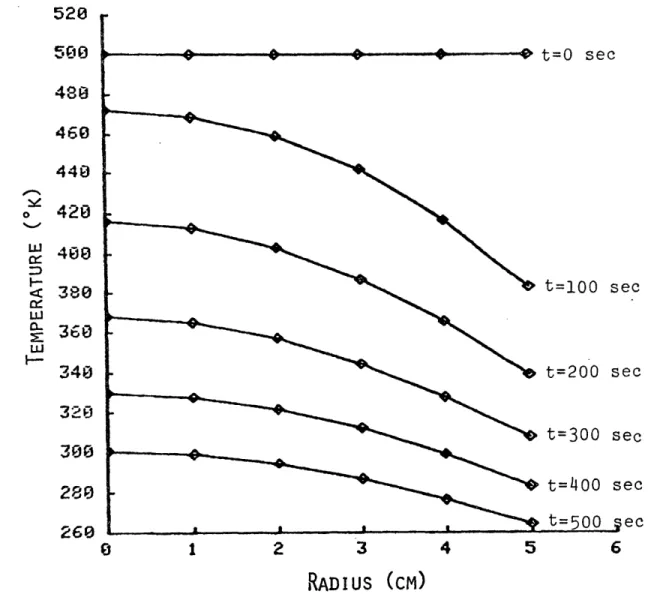
The purpose of the first case was to test the method

in which the conduction equations are finite differenced

and solved, so a de-emphasis was placed on the boundary

conditions. In fact, the geometry used in this case is a

solid cylinder of 5.0 cm radius, so the inner boundary

con-dition is adiabatic, and the heat flux apportioning scheme

is bypassed. The situation modeled is that of a cylinder

at 500°k placed in a 200°k environment, with a constant

heat transfer coefficient of 342.06W/m2°k on the outer

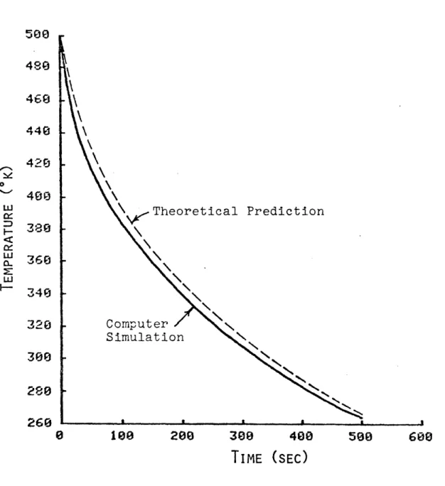
boundary. The calculations were continued for 500 seconds,

using ten second time steps. The results are plotted in

Figure 3.4. The temperature histories at the center and

surface of the cylinder were then compared with the

ana-lytical solutions [5]. The results of this comparison are

displayed in Figures 3.5 and 3.6. As one can see, the model

simulates the analytical results quite closely. If a smaller

(68)

-57-0 1 2 3 4 5 6

RADIUS (CM)

Figure 3.4 Temperature Distribution of Cylinder Initially at 500°k, Placed in a 200°k Environment

C>

L..

in 500 480 460 440 o 428 uJ 400 w <C 380 L

w

£ 360

w

LLi

340

320

300

280 2;o

ec ec ec ec ec

(69)

0 100 200 300 400 500

TIME (SEC)

Figure 3.5 Centerline Temperature of Cylinder vs. Theoretical Prediction .Juu