Rapid dynamic activation of a marine-based
Arctic ice cap
Malcolm McMillan1, Andrew Shepherd1,2, Noel Gourmelen3, Amaury Dehecq4, Amber Leeson1, Andrew Ridout2, Thomas Flament1, Anna Hogg1, Lin Gilbert2, Toby Benham5, Michiel van den Broeke6, Julian A. Dowdeswell5, Xavier Fettweis7, Brice Noël6, and Tazio Strozzi8
1
Centre for Polar Observation and Modelling, University of Leeds, Leeds, UK,2Centre for Polar Observation and Modelling, University College London, London, UK,3School of Geosciences, University of Edinburgh, Edinburgh, UK,4The Computer Science, Systems, Information and Knowledge Processing Laboratory, Université de Savoie, Chambéry, France,5Scott Polar Research Institute, University of Cambridge, Cambridge, UK,6Institute for Marine and Atmospheric Research, Utrecht University, Utrecht, Netherlands,7Department of Geography, University of Liège, Liège, Belgium,8GAMMA Remote Sensing Research and Consulting AG, Gümligen, Switzerland
Abstract
We use satellite observations to document rapid acceleration and ice loss from a formerly slow-flowing, marine-based sector of Austfonna, the largest ice cap in the Eurasian Arctic. During the past two decades, the sector ice discharge has increased 45-fold, the velocity regime has switched from predominantly slow (~ 101m/yr) to fast (~ 103m/yr)flow, and rates of ice thinning have exceeded 25 m/yr. At the time of widespread dynamic activation, parts of the terminus may have been nearfloatation. Subsequently, the imbalance has propagated 50 km inland to within 8 km of the ice cap summit. Our observations demonstrate the ability of slow-flowing ice to mobilize and quickly transmit the dynamic imbalance inland; a process that we show has initiated rapid ice loss to the ocean and redistribution of ice mass to locations more susceptible to melt, yet which remains poorly understood.1. Introduction
Ice caps and glaciers separate from the Greenland and Antarctic ice sheets have contributed approximately one third of recent sea level rise [Gardner et al., 2013]. Models project continued ice loss from these systems throughout the 21st century under climate warming scenarios [Radic and Hock, 2011; Marzeion et al., 2012; Meier et al., 2007], although the future dynamic response of marine-terminating sectors remains highly uncertain [Pfeffer et al., 2008]. In Greenland and Antarctica, changing boundary conditions have driven rapid velocityfluctuations of fast-flowing marine-based glaciers [Holland et al., 2008; Nick et al., 2009; Joughin et al., 2012]. Changes in the dynamics of marine-terminating ice streams of a Russian Arctic ice cap have also been observed [Moholdt et al., 2012], demonstrating the high variability in ice discharge from these fast-flowing systems. In contrast, the capacity of slow-flowing ice to become dynamically active and to rapidly contribute ice mass to the ocean remains poorly understood.
The largest contribution from glaciers and ice caps to sea level rise, considering surface mass balance alone, is projected to come from the Arctic [Radic and Hock, 2011], where recent atmospheric warming has been particularly strong [Bekryaev et al., 2010]. Smaller bodies of ice in these regions, such as Arctic ice caps (104–105km2), exhibit regions of fast and slowflow and are potentially more exposed to changing climatic conditions than the larger ice sheets of Greenland and Antarctica. Continued monitoring of these smaller ice masses not only constrains their ongoing contribution to sea level rise but also provides analogies for anticipated changes within larger ice sheet settings [Joughin et al., 2014]. This study documents rapid ice loss from a marine-based sector of Austfonna, the largest ice cap in the Eurasian Arctic. Using observations from eight satellite missions, we present a two decade record of ice mass and velocityfluctuations and investigate the development of widespread dynamic imbalance within this region.
2. Study Area
Austfonna is located in northeastern Svalbard. Containing approximately 2500 km3of ice, it is drained by both land- and marine-terminating glacier systems [Dowdeswell et al., 2008]. About 28% of the ice cap bed lies below sea level and over 200 km of its southern and eastern margin terminates in the ocean [Dowdeswell,
Geophysical Research Letters
RESEARCH LETTER
10.1002/2014GL062255
Key Points:
• Recent dynamic activation of a formerly slow-flowing marine Arctic ice cap • Imbalance has spread 50 km inland to
within 8 km of the ice cap summit • Ice discharge has increased 45-fold, and
thinning rates have exceeded 25 m/yr
Supporting Information:
• Readme
• Table S1 and Figures S1–S4
Correspondence to:
M. McMillan,
Citation:
McMillan, M., et al. (2014), Rapid dynamic activation of a marine-based Arctic ice cap, Geophys. Res. Lett., 41, 8902–8909, doi:10.1002/2014GL062255. Received 27 OCT 2014
Accepted 26 NOV 2014
Accepted article online 2 DEC 2014 Published online 23 DEC 2014
This is an open access article under the terms of the Creative Commons Attribution License, which permits use, distribution and reproduction in any medium, provided the original work is properly cited.
1986; Dowdeswell et al., 2008], with parts resting on a retrograde slope. During the 1990s and 2000s, increased transport of Atlantic Water into the Barents Sea has been accompanied by a northward retreat of sea ice [Smedsrud et al., 2013]. Model simulations of atmospheric conditions over the same period suggest no statistically significant trend in summer warming over this region, because of the increased frequency of northerly atmosphericflows associated with negative phases of the North Atlantic Oscillation [Fettweis et al., 2013a]. Repeat airborne [Bamber et al., 2004] and satellite [Moholdt et al., 2010] altimetry measurements have recorded slight thickening (up to 0.5 m/yr) of the ice cap interior and moderate thinning (1–3 m/yr) at its margin. The majority of Austfonnaflows slowly (typically below 25 m/yr) [Dowdeswell et al., 2008], although isolated units of fasterflow do exist. Historical records indicate episodic glacier surges lasting 3–10 years in some sectors [Schytt, 1969; Dowdeswell et al., 1991; Hagen et al., 1993], and marine surveys off the eastern shore suggest past ice margin instability [Robinson and Dowdeswell, 2011]. In the southeast, observations have revealed summertime acceleration of a 1160 km2region (hereafter basin 3 [Dowdeswell, 1986]) linked to the supply of meltwater to the subglacial system [Dunse et al., 2012].
3. Data and Methods
We computed decadal elevation and velocity changes of Austfonna using repeat satellite altimeter and synthetic aperture radar (SAR) measurements. Rates of elevation change were estimated between 2002 and 2014 by applying along-track processing algorithms [Smith et al., 2009; Flament and Remy, 2012; McMillan et al., 2014] to altimetry data acquired by the Envisat (2002–2010), ICESat (2003–2009), and CryoSat (2010–2014) satellites (see supporting information). Elevation measurements acquired over a succession of orbit cycles were grouped either within along-track segments (Envisat and ICESat) or 2–5 km square geographic regions (CryoSat), and these data were then used to estimate spatial and temporal rates of elevation change. For the period 2010–2014, when comprehensive (>96% coverage at 5 km grid spacing) surveying of basin 3 was achieved, we estimated changes in ice volume for this sector by spatially integrating estimates of surface elevation change and assigning the mean basin elevation rate to the remaining (<4%) unobserved areas. We then computed mass change by assuming a dynamic origin to the imbalance and assigning volume loss to be at a density of ice. Uncertainties were computed from each modelfit, summed within each region, and converted to mass equivalent using a density of ice. Ice velocity and discharge were mapped using synthetic aperture radar (SAR) interferometry and feature tracking, with data acquired by the European Remote Sensing (ERS-1 and ERS-2) satellites, the Advanced Land Observing Satellite (ALOS), and the TerraSAR-X and Sentinel-1a satellites (see supporting information). At each time period, discharge was computed across aflux gate positioned close to the ice front, where the glacier thickness had been surveyed previously by radio echo sounding [Dowdeswell, 1986] and adjusted for subsequent thinning using the altimetry data. Glacier discharge was combined with annual surface mass balance estimates from the Regional Atmospheric Climate Model (RACMO2) [van Angelen et al., 2013] and the Modèle Atmosphérique Régional (MAR) [Fettweis et al., 2013b] to estimate net ice mass balance upstream of theflux gate. Ice discharge uncertainties were assumed to be 5% of the recorded discharge, based on analysis of the residual displacements measured over stable ground, and the variance of repeat measurements of ice thickness at survey crossing points. Surface mass balance uncertainty was taken as the standard deviation of the annual MAR and RACMO2 predictions, therefore reflecting the intermodel consistency of the simulations.
In addition to the altimetry and SAR observations, we used several other supporting data sets in our analysis (see supporting information). Calving front locations were digitized from SAR data, and sea ice extent was mapped using daily sea ice concentration data from the National Snow and Ice Data Centre (www.nsidc.org). Annual surface mass balance and runoff estimates were compiled from daily MAR [Fettweis et al., 2013b] and RACMO2 [van Angelen et al., 2013] simulations.
4. Results
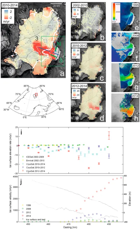
Between 2003 and 2009, repeat altimetry measurements indicate localized surface lowering at the terminus of basin 3, with rates exceeding 5.0 ± 0.4 m/yr in places (Figure 1). Concurrently, SAR estimates of ice velocity show changes in iceflow close to the margin of this sector. In 1995, the basin had been predominantly slowflowing, except for a single flow unit to the north achieving a maximum speed of 150 ± 6 m/yr. Observations
Figure 1. Austfonna surface elevation change and velocity, 1995–2014. Surface elevation change from (a, c, and d) CryoSat and (b) Envisat (2002–2010) and ICESat (2003–2009). Ice flow velocity from (e) ERS-1/2, (f) ALOS, (g) TerraSAR-X, and (h) TerraSAR-X and Sentinel-1a combination. (i, j) Surface elevation change and velocity along a longitudinal profile. In Figure 1a, elevation rates are computed on a 2 km square grid and smoothed using a 6 km square medianfilter. The black dots delineate the boundaries of drainage basins [Dowdeswell, 1986], and basin 3 is labeled. Bed elevation contours [Dowdeswell, 1986] at 100 m intervals are shown in white, with the thick line being 0 m above sea level, the blue line locates the transect in Figures 1i and 1j, and the green lines mark the north (N) and south (S) profiles in Figure 3. The green box indicates the area covered by Figures 1e–1h. In Figure 1e, the white line marks the flux gate used to estimate glacier discharge. The background image is a backscatter intensity image acquired by Sentinel-1a on 18 April 2014. In Figure 1i, elevation rates have been averaged over 10 km north-south strips to capture behavior across the glacier width. In Figure 1j, spaced grey dots indicate intermittent or absent airborne survey data of the ice and bedrock surface, and ice velocity decreases close to the terminus in 2012 because fastflow has yet to develop across the full glacier width. The current terminus position is at 497.8 km east.
from 2008 showed that thisflow unit had accelerated by a factor of 5 and widened, and also identified a new area of fastflow to the south, where ice thinning was most pronounced. After 2009, rates of ice thinning intensified and spread inland to encompass the entire drainage basin, resulting in an average thinning rate of 2.9 ± 0.5 m/yr between 2010 and 2014. Since 2012, thinning has been exceptionally high across the basin—averaging and peaking at 5.5 ± 0.8 m/yr and 29 ± 1 m/yr, respectively—although there is now evidence of localized thickening at the terminus (Figure 1d). In parallel, the regime of iceflow has recently altered significantly, with the two distinct flow units merging to form a single stream of fast flow across the full basin width. By 2014, we detect maximum iceflow speeds of 3800 ± 3 m/yr, representing a 25-fold increase on the maximum measured in 1995. Both the magnitude and pattern of the observed velocity evolution are broadly consistent with a shorter-period, higher-frequency record derived from SAR data acquired during 2012–2013 [Dunse et al., 2014].
The observed changes indicate recent ice mass loss from basin 3, which we assessed using the altimeter and SAR measurements (Figure 2). The regular altimeter sampling is well suited to deriving multiyear trends in ice loss, whereas the episodic estimates of daily to monthly displacement provided by SAR acquisitions better capture the evolution of ice discharge, albeit computed over much shorter time periods. For ease of comparison, we have converted SAR-derived estimates to annual equivalent discharge rates. The SAR measurements indicate that in 2008 basin 3 remained broadly in balance. Since then the ice imbalance has increased substantially. In February 2014, for example, ice discharge across the defined flux gate was
Figure 2. Temporal evolution of basin 3 and its surrounding environment. (a) Mass imbalance from SAR and atmospheric modeling (input-output method, IOM) and repeat altimetry, the calving front location (relative to 1981, negative indicates retreat) and surface mass balance. Mass imbalance is computed directly from the IOM and altimetry methods and has not been adjusted for mass retention due to terminus advance. Percentage of late-season (July–November) days with sea ice cover, averaged over the periods (b) 1992–2011 and (c) 2012–2013, with the red dot marking Austfonna. (d, e) Modeled annual surface meltwater runoff, together with the long-term mean and standard deviation (SD), computed from MAR and RACMO2 simulations. The green dashed line indicates the long-term (1960–2013) trend. (f, g) Latitudinal limit of late-season (July–November) sea ice coverage, defined to be the limit at which there was sea ice coverage on a minimum of 30% of days. The data were generated from annual maps of the percentage days exhibiting sea ice cover and plotted as the average latitude at which the 30% contour crossed the 25°E and 35°E meridians. The grey line indicates the latitude of basin 3, and the green dashed line indicates the long-term (1992–2013) trend.
equivalent to 8.7 ± 0.4 Gt/yr, compared to an average modeled surface mass balance input of only 0.4 ± 0.1 Gt/yr. To compute longer-term average rates of imbalance, we used the 5 km CryoSat elevation change measurements, which provide comprehensive (>96%) coverage of basin 3 from 2010 onward. We estimated that the rate of ice loss increased from 1.5 ± 0.6 Gt/yr between July 2010 and May 2012 to 5.9 ± 0.9 Gt/yr between June 2012 and April 2014. These mass loss estimates do not directly account for migration of the calving front, which either preserves ice mass within the glacier system or yields increased ice loss to the ocean. Since 2010, there has been a net advance of the terminus of approximately 50 km2, which we estimate to have retained a total of 3.7 ± 1.1 Gt of the ice leaving the upstream catchment (see supporting information).
5. Discussion
Episodic surges of Austfonna basins have been previously documented [Schytt, 1969; Dowdeswell et al., 1991; Hagen et al., 1993] and are typically understood to be triggered by internal processes rather than external forcing. While an internally generated surge mechanism may be responsible for the glacier evolution we have recorded, there are several aspects that may suggest the influence of alternative factors. First, although the temporal sampling offered by our repeat SAR measurements does not provide a continuous account of the basin evolution, it does appear that glacier velocities have broadly increased over a period of 20 years, which is more than twice the duration of any previous surge event, inclusive of the deceleration phase [Dowdeswell et al., 1991]. Second, our observations suggest that acceleration and thinning may have initiated at the glacier terminus (Figures 1b and 1f ) and acceleration occurred at a time when the ice front was either stable or in retreat. Such behavior is atypical of surge evolution and more reminiscent of a response to changing boundary conditions at the terminus [Nick et al., 2009]. Third, the imbalance has developed at a time of significant climatic change in the Arctic and is redolent of changes that have occurred at other marine-terminating glaciers that have experienced external forcing [Holland et al., 2008]. Finally, we note that the distinction between a surge and an externally forced process may not be straightforward in cases where the glacier geometry or rheology is changing in response to its surrounding climate [Dowdeswell et al., 1995]; indeed, the two largest surges recorded in Svalbard occurred within a 2 year period during the 1930s [Schytt, 1969; Hagen et al., 1993] at a time of sustained atmospheric and oceanic warming [Polyakov et al., 2013].
We investigated regional climatic variations (Figure 2) to assess the extent to which they may relate to the observed changes in ice velocity and thickness. Atmospheric warming holds the potential to influence ice dynamics through processes of meltwater lubrication [Zwally et al., 2002], ice and bed warming [Phillips et al., 2013; Dunse et al., 2014], or alteration of glacier geometry. Additionally, melt-induced thinning or retreat, either by the atmosphere or the ocean, may initiate a dynamic response by reducing resistive stresses at the ice base [Pfeffer, 2007; Joughin et al., 2014]. We therefore examined model simulations of meltwater runoff [Fettweis et al., 2013b; van Angelen et al., 2013], together with satellite observations of sea ice extent, which have been shown to be correlated withfluctuations in ocean heat in this region [Schlichtholz, 2011; Arthun et al., 2012]. The basin-integrated surface mass balance has been predominantly positive over recent decades (Figure 2a), and there is no indication of anomalously high runoff in recent years, with the exception of 2013 (Figures 2d and 2e), by which time the imbalance was well established. Thesefindings are supported by previous studies [Fettweis et al., 2013a] that, excluding 2013, found no statistically significant trend in summer warming over Svalbard during the last two decades. They are also consistent with our glaciological observations, with the ice margin thinning, acceleration and retreat that occurred prior to 2012 appearing to better match the response expected from changing conditions at the terminus, rather than from the enhanced inland delivery of surface melt water to the ice cap base [Nick et al., 2009]. In this sense, we do notfind in our data further support for a proposed activation mechanism related to the increased delivery of surface melt water to the ice cap base [Dunse et al., 2014], although it remains possible that smaller incremental changes in subglacial meltwater delivery could eventually trigger a dynamic response.
There is evidence that ocean conditions in the Barents Sea have changed in recent years, both from oceanographic surveys [Polyakov et al., 2005, 2013] and the recorded sea ice extent [Schlichtholz, 2011; Arthun et al., 2012]. Given the observed correlation between these two factors [Schlichtholz, 2011; Arthun et al., 2012], we investigated changing ocean conditions by computing interannual variations in the period of sea ice cover (Figures 2b and 2c) and also characterized its northward migration by tracking the lateral extent of
Arctic sea ice in the western Barents Sea (Figures 2f and 2g). These data indicate a marked reduction in the duration of late-season sea ice cover east of Austfonna in recent years, which can be attributed to the observed inflow of warm Atlantic Water into the Barents Sea causing the delayed onset of winter sea ice formation [Polyakov et al., 2005; Smedsrud et al., 2013]. In particular,
measurements from an oceanographic survey in 2004 identified a pulse of
anomalously warm Atlantic Water offshore of Austfonna [Polyakov et al., 2013]. Subsequent repeat observations showed that the warming associated with this intrusion peaked between 2006 and 2008, with upper ocean temperatures approximately 4°C above the 40 year mean [Polyakov et al., 2013]. These temperatures were the highest ever recorded in this region [Polyakov et al., 2005, 2013], providing the potential for substantially enhanced ocean melting at marine-terminating sectors of Austfonna. Despite the apparent coincidence between increased offshore ocean temperatures and the dynamic activation of basin 3, the lack of more extensive oceanographic and glaciological measurements
prevents a direct causal link from being definitively established or discounted. The existing measurements do, however, allow us to explore possible geometrical configurations of the terminus prior to the widespread activation of this sector in 2012. At this time, ice thinning and acceleration were focused on two individualflow units (Figure 1) and although localized had been sustained for several years. Airborne radio echo soundingflight lines from 1983 provide longitudinal transects across these two regions (see supporting information). These data show that the terminus rested on bedrock 50–100 m below sea level, with an ice cliff extending 25–80 m above sea level (Figure 3). To estimate the subsequent evolution of the terminus geometry, we temporally integrated our 2003–2012 elevation rate estimates at the locations of the north and south units of fastflow (Figure 1). Prior to these measurements—for the period 1983 to 2003—we estimated a total of 15 m of surface lowering, from a comparison of near terminus radio echo sounding and ICESat elevation data (see supporting information).
Based on the observed ice thinning, we then estimated the 2012 terminus geometry of the twoflow units, assuming that the ice, once sufficiently thin, floats in hydrostatic equilibrium. This analysis suggests that the sustained ice thinning observed prior to 2012 may have been sufficient for kilometer-scale sections of the terminus to reachflotation, leading to partial ungrounding of the glacier from the underlying bed (Figure 3). In the central terminus region of basin 3, however, the thicker ice and absence of sustained thinning prior to 2012 would have prevented terminus ungrounding, meaning that anyfloatation was unlikely to have been universal across the entire calving front (see supporting information). Without more extensive measurements from this time, it is unclear exactly which part of the terminus may have achieved buoyancy, and
Figure 3. Geometry of the glacier terminus. The terminus geometry along two airborneflight lines (Figure 1) in 1983 (observed) and in 2012 (estimated). The grounding line position is determined as the location where the modeled surface elevation intersects theflotation profile, computed from the bed elevation and assuming, conservatively, a solid ice column with density 917 kg m 3. The dashed lines indicate extrapolation beyond the limits of the radio echo sounding data, byfixing the surface and bed elevations at their most seaward values. The thickness of the shaded areas represents the height of the ice surface aboveflotation. In 1983 the ice cap was well grounded with the surface elevation being substantially in excess of theflotation profile (light shading). By 2012, a 1 km section of the terminus may have reachedflotation in both the northern and southern parts of this sector (dark shading).
whether the associated reduction in resistive stresses, with its capacity to drive further thinning and acceleration [Nick et al., 2009; Pfeffer, 2007], could have mobilized the entire basin. As such, this analysis does not establish a direct causal link between ocean forcing, terminus thinning, and dynamic activation nor does it provide a process-based argument for such a mechanism. However, it does demonstrate that based upon the available data it is possible that when widespread dynamic activation occurred in 2012, a portion of the terminus may have reached buoyancy.
6. Conclusions
To date, the observed dynamical imbalance has propagated 50 km inland to within 8 km of the ice cap summit, producing widespread ice loss to the ocean. Currently, the glacier terminus rests on a broadly undulating bed; however, farther inland the bed deepens, providing the potential for future instability if further ungrounding occurs [Schoof, 2007]. The imbalance could have been triggered by a number of processes, including an internally generated surge, increased meltwater availability at the bed [Dunse et al., 2014], or enhanced ocean- or atmosphere-driven melting at the terminus; indeed, a combination of factors may have contributed [Nick et al., 2009; Jenkins, 2011]. Across Austfonna, however, there is a coherent pattern of ice margin thinning at all marine-based sectors, which is not apparent at land-terminating basins (Figure 1). This may suggest either a common ocean forcing or the influence of bed conditions specific to marine settings. Additional evidence of anomalously warm waters offshore [Polyakov et al., 2005, 2013] and insignificantly increased atmospheric melting in recent years leads us to favor the former mechanism, rather than one linked to increased melt water delivery to the bed, although a definitive link would require dynamical modeling and measurements at the calving front. Until then, it is unclear whether the moderate rates of thinning of other marine ice sectors are a prelude to similar widespread mass loss in these areas, or whether the large dynamical imbalance at basin 3 will be sustained over time. Nonetheless, the behavior recorded here demonstrates that slow-flowing ice caps can enter states of significant imbalance over very short timescales and highlights their capacity for increased ice loss in the future.
References
Arthun, M., T. Eldevik, L. H. Smedsrud, Ø. Skagseth, and R. B. Ingvaldsen (2012), Quantifying the influence of Atlantic heat on Barents Sea ice variability and retreat, J. Clim., 25, 4736–4743.
Bamber, J., W. Krabill, V. Raper, and J. Dowdeswell (2004), Anomalous recent growth of part of a large Arctic ice cap: Austfonna, Svalbard, Geophys. Res. Lett., 31, L12402, doi:10.1029/2004GL019667.
Bekryaev, R. V., I. V. Polyakov, and V. A. Alexeev (2010), Role of polar amplification in long-term surface air temperature variations and modern Arctic warming, J. Clim., 23(14), 3888–3906.
Dowdeswell, J. A. (1986), Drainage-basin characteristics of Nordaustlandet ice caps, Svalbard, J. Glaciol., 32, 31–38.
Dowdeswell, J. A., G. S. Hamilton, and J. O. Hagen (1991), The duration of the active phase on surge-type glaciers: Contrasts between Svalbard and other regions, J. Glaciol., 37, 127.
Dowdeswell, J. A., R. Hodgkins, A.-M. Nuttall, J. O. Hagen, and G. S. Hamilton (1995), Mass balance change as a control on the frequency and occurrence of glacier surges in Svalbard, Norwegian High Arctic, Geophys. Res. Lett., 22, 2909–2912, doi:10.1029/95GL02821.
Dowdeswell, J. A., T. J. Benham, T. Strozzi, and J. O. Hagen (2008), Iceberg calvingflux and mass balance of the Austfonna ice cap on Nordaustlandet, Svalbard, J. Geophys. Res., 113, F03022, doi:10.1029/2007JF000905.
Dunse, T., T. V. Schuler, J. O. Hagen, and C. H. Reijmer (2012), Seasonal speed-up of two outlet glaciers of Austfonna, Svalbard, inferred from continuous GPS measurements, Cryosphere, 6, 453–466.
Dunse, T., T. Schellenberger, A. Kaab, J. O. Hagen, T. V. Schuler, and C. H. Reijmer (2014), Destabilisation of an Arctic ice cap triggered by a hydro-thermodynamic feedback to summer-melt, Cryosphere Discuss., 8, 2685–2719.
Fettweis, X., B. Franco, M. Tedesco, J. H. van Angelen, J. T. M. Lenaerts, M. R. van den Broeke, and H. Gallée (2013a), Estimating the Greenland ice sheet surface mass balance contribution to future sea level rise using the regional atmospheric climate model MAR, Cryosphere, 7, 469–489. Fettweis, X., E. Hanna, C. Lang, A. Belleflamme, M. Erpicum, and H. Gallée (2013b), Important role of the mid-tropospheric atmospheric
circulation in the recent surface melt increase over the Greenland ice sheet, Cryosphere, 7, 241–248.
Flament, T., and F. Remy (2012), Dynamic thinning of Antarctic glaciers from along-track repeat radar altimetry, J. Glaciol., 58(211), 830–840. Gardner, A. S., et al. (2013), A reconciled estimate of glacier contributions to sea level rise: 2003 to 2009, Science, 340(6134), 852–857. Hagen, J. O., O. Liestøl, E. Roland, and T. Jørgensen (1993), Glacier Atlas of Svalbard and Jan Mayen, Meddelelser, vol. 129, Norsk Polarinstitutt, Oslo. Holland, D. M., R. H. Thomas, B. de Young, M. H. Ribergaard, and B. Lyberth (2008), Acceleration of Jakobshavn Isbræ triggered by warm
subsurface ocean waters, Nat. Geosci., 1, 659–664.
Jenkins, A. (2011), Convection-driven melting near the grounding lines of ice shelves and tidewater glaciers, J. Phys. Oceanogr., 41, 2279–2294. Joughin, I., R. B. Alley, and D. M. Holland (2012), Ice-sheet response to oceanic forcing, Science, 338, 1172.
Joughin, I., B. E. Smith, and B. Medley (2014), Marine ice sheet collapse potentially under way for the Thwaites Glacier Basin, West Antarctica, Science, 344, 735.
Marzeion, B., A. H. Jarosch, and M. Hofer (2012), Past and future sea-level change from the surface mass balance of glaciers, Cryosphere, 6, 1295–1322.
McMillan, M., A. Shepherd, A. Sundal, K. Briggs, A. Muir, A. Ridout, A. Hogg, and D. Wingham (2014), Increased ice losses from Antarctica detected by CryoSat-2, Geophys. Res. Lett., 41, 3899–3905, doi:10.1002/2014GL060111.
Acknowledgments
This work was supported by the UK Natural Environment Research Council. The satellite altimetry data used in this study are freely available from the European Space Agency (https://earth. esa.int/web/guest/data-access) and the National Snow and Ice Data Centre (http://nsidc.org/data/icesat/). The SAR data are available from the European Space Agency (https://earth.esa.int/ web/guest/data-access), the Japanese Space Agency (http://www.eorc.jaxa.jp/ ALOS/en/ra/ra4_guide.htm) and the German Aeronautics and Space Research Centre (http://sss.terrasar-x. dlr.de/). Sea ice data are available from the National Snow and Ice Data Centre (http://nsidc.org/data/seaice/). We are grateful to Geir Moholdt for providing a digital elevation model of Austfonna and to the Editor and three anonymous reviewers for their comments. The Editor thanks three anonymous reviewers for their assistance in evaluating this paper.
Meier, M. F., M. B. Dyurgerov, U. K. Rick, S. O’Neel, W. Tad Pfeffer, R. S. Anderson, S. P. Anderson, and A. F. Glazovsky (2007), Glaciers dominate Eustatic sea-level rise in the 21st century, Science, 317(5841), 1064–1067.
Moholdt, G., J. O. Hagen, T. Eiken, and T. V. Schuler (2010), Geometric changes and mass balance of the Austfonna ice cap, Svalbard, Cryosphere, 4, 2134.
Moholdt, G., T. Heid, T. J. Benham, and J. A. Dowdeswell (2012), Dynamic instability of marine-terminating glacier basins of Academy of Sciences Ice Cap, Russian High Arctic, Ann. Glaciol., 53, 193–201.
Nick, F. M., A. Vieli, I. M. Howat, and I. Joughin (2009), Large-scale changes in Greenland outlet glacier dynamics triggered at the terminus, Nat. Geosci., 2, 110–114.
Pfeffer, W. T. (2007), A simple mechanism for irreversible tidewater glacier retreat, J. Geophys. Res., 112, F03S25, doi:10.1029/2006JF000590. Pfeffer, W. T., J. T. Harper, and S. O’Neel (2008), Kinematic constraints on glacier contributions to 21st-century sea-level rise, Science, 321, 1340. Phillips, T., H. Rajaram, W. Colgan, K. Steffen, and W. Abdalati (2013), Evaluation of cryo-hydrologic warming as an explanation for increased
ice velocities in the wet snow zone, Sermeq Avannarleq, West Greenland, J. Geophys. Res. Earth Surf., 118, 1241–1256, doi:10.1002/ jgrf.20079.
Polyakov, I. V., et al. (2005), One more step toward a warmer Arctic, Geophys. Res. Lett., 32, L17605, doi:10.1029/2005GL023740. Polyakov, I. V., U. S. Bhatt, J. E. Walsh, E. Povl Abrahamsen, A. V. Pnyushkov, and P. F. Wassmann (2013), Recent oceanic changes in the Arctic
in the context of long-term observations, Ecol. Appl., 23, 1745–1764.
Radic, V., and R. Hock (2011), Regionally differentiated contribution of mountain glaciers and ice caps to future sea-level rise, Nat. Geosci., 4, 91–94.
Robinson, P., and J. A. Dowdeswell (2011), Submarine landforms and the behavior of a surging ice cap since the last glacial maximum: The open-marine setting of eastern Austfonna, Svalbard, Mar. Geol., 286, 82–94.
Schlichtholz, P. (2011), Influence of oceanic heat variability on sea ice anomalies in the Nordic Seas, Geophys. Res. Lett., 38, L05705, doi:10.1029/2010GL045894.
Schoof, C. (2007), Ice sheet grounding line dynamics: Steady states, stability, and hysteresis, J. Geophys. Res., 112, F03S28, doi:10.1029/ 2006JF000664.
Schytt, V. (1969), Some comments on glacier surges in eastern Svalbard, Can. J. Earth Sci., 6(4), 867–873.
Smedsrud, L. H., et al. (2013), The role of the Barents Sea in the Arctic climate system, Rev. Geophys., 51, 415–449, doi:10.1002/rog.20017. Smith, B. E., H. A. Fricker, I. R. Joughin, and S. Tulaczyk (2009), An inventory of active subglacial lakes in Antarctica detected by ICESat
(2003–2008), J. Glaciol., 55(192), 573–595.
van Angelen, J. H., M. R. van den Broeke, B. Wouters, and J. T. M. Lenaerts (2013), Contemporary (1960–2012) evolution of the climate and surface mass balance of the Greenland ice sheet, Surv. Geophys., doi:10.1007/s10712-013-9261-z.
Zwally, H. J., W. Abdalati, T. Herring, K. Larson, J. Saba, and K. Steffen (2002), Surface melt-induced acceleration of Greenland Ice-Sheetflow, Science, 297(5579), 218–222.