Diesel engine instantaneous oil consumption measurements using the sulfur dioxide tracer technique

Diesel Engine Instantaneous Oil Consumption Measurements Using the Sulfur

Dioxide Tracer Technique

by

Douglas M. Schofield

B. S., Marine Engineering and Naval Architecture; United States Coast Guard Academy, 1991

Submitted to the Departments of Ocean Engineering and Mechanical Engineering in

Partial Fulfillment of the Requirements for the Degrees of

MASTER OF SCIENCE IN NAVAL ARCHITECTURE AND MARINE

ENGINEERING

and

MASTER OF SCIENCE IN MECHANICAL ENGINEERING

at the

Massachusetts Institute of Technology; May 1995

© 1995 Douglas M. Schofield. All rights reserved.

The author hereby grants to MIT permission to reproduce and to distribute publicly paper

and electronic copies of this doqument in whole or in part.

Signature of Author

Certified by

Certified by

-,Dep#artment of Ocean Engintering May 1995

Dr. Alan J. Brown

Profe'ssor, Department of Ocean Engineering

Thesis Reader

Dr2Aictor W. Wong

Lecturer, Department of Mechanical Engineering

Thsis Advisor

v *

~~~~-

-g

eg7

Accepted by

-'---

A. Douglas

Carmichae,

Chairman

Departmental Committee on Graduate Studies

Departnme.Qoef-Qqn Engineering

MASSACHUS;TTS INSTITUTE OF TECHNOLOGY

JUL 2

8

1995

A. A. Sonin, Chairman

Departmental Committee on Graduate Studies

Department of Mechanical Engineering

Accepted by

__Y__ I_ __ · )__I___

Diesel Engine Instantaneous Oil Consumption Measurements Using the Sulfur Dioxide Tracer Technique

by

Douglas M. Schofield

Submitted to the Department of Ocean Engineering and the Department of Mechanical Engineering in Partial Fulfillment of the Requirements for the Degrees of Master of Science in Naval Architecture and Marine Engineering and Master of Science in Mechanical Engineering.

ABSTRACT

A study of the oil consumption characteristics was completed using a single cylinder direct injection diesel engine. The objectives included establishing the testing procedures for a real-time sulfur dioxide oil consumption system and studying the ring-pack derived oil consumption including testing the repeatability and variability through load changes, speed changes, and changes in oil control ring tension. Also, the use of a commercially available oil was investigated to determine its effectiveness in a sulfur dioxide testing apparatus.

The testing included three test matrices all completed at steady-state engine operating conditions. The first had two loading conditions through three speeds while continuously monitoring the ring-pack oil consumption. This matrix had 24 tests while using a standard oil control ring. The second had the same two loading conditions through two speeds while continuously monitoring only the ring-pack oil

consumption. This matrix had 22 tests using an oil control ring with 45% less tension than the standard configuration. The third matrix had two loading conditions through two speeds with 12 tests. This matrix measured the entire engine oil consumption through the same apparatus, but the engine oil was a commercially available 10W-30 grade oil.

Several conclusions were drawn from the data analysis. The first matrix showed that the oil consumption data was repeatable from test to test for the high and low speed, but the mid-range speed showed oil consumption variability with different oil consumption plateaus lasting between 15 and 30 minutes with changes in oil consumption among these plateaus as much i00%. These plateaus may be caused by the axial and rotational dynamics of the piston rings. The second matrix results showed larger variability with instantaneous spiking of the oil consumption occurring during the continously monitored real-time oil consumption. These spikes were the rapid rising and falling of oil consumption with increases as much as 500% and often periodic in behavior with periods from 2 to 20 minutes. The instantaneous spikes may be caused by ring-pack reverse blow-by gases, transporting oil into the cylinder combustion region. Together, the analyses showed that by decreasing the oil control ring tension by 45%, the mostly ring-pack derived oil consumption did not change significantly at low speed but increased by 63% at the maximum speed. Also, by decreasing the oil control ring tension, more variability in the mostly ring-pack derived oil consumption values were seen. The third matrix showed that this sulfur dioxide system was sensitive enough to determine the oil consumption values at the 1200 and 2400 rpm using a commercially available 10W-30 oil.

Thesis Supervisor: Victor W. Wong

Title: Lecturer, Department of Mechanical Engineering Thesis Reader: Alan J. Brown

ACKNOWLEDGMENTS

The success of this project was by no means an individual effort. I was given support from many people, and I would like to sincerely thank them all.

Eric Ford has contributed a lot to this project. His patience and attitude made

working together easy and fun. His organization and devotion to the task at hand

influenced all people involved in the process.

My advisors, Captain Brown and Dr. Wong, both provided the efficient means in

which to complete the current study. Other faculty members at MIT gave crucial comments and guidance in the successful completion of this thesis. Their guidance and support were extremely beneficial; I thank you all.

Dr. Alan Bentz of the USCG R&D Center was a critical asset to the project. His

financial support and chemistry technical advice were invaluable. His guidance has not only made my research go smoothly, but has also supported many other Coast Guard and

Naval Officers here at MIT.

Richard Flaherty at Cummins Engine Company gave many hours of his time in

setting up the oil consumption system. His patience and determination of the project were

most valuable. Throughout the entire extended dyno repair period, he continued to push

forward, making the project meet its deadline. He was truly a mentor, whom I would feel

honored to work for in the future.

Many others contributed efforts towards this project. David Fiedler of Dana

Perfect Circle, Philip Burnett of Shell Oil, and Norbert Abraham of Cummins Engine

Company, all contributed critical pieces to the overall project.

The members of the Sloan Lab Staff also deserve recognition. Don Fitzgerald gave excellent technical and ordering support. Nancy Cook gave important administrative

assistance. Brian Corkum gave excellent "hands-on" guidance and skill. His devotion to

always teaching new students the tools and methods of the lab is irreplaceable. Without

Office mates and friends always make projects go a little easier. R.B., Erik, Brigitte, Dan, Rob, Mark, Lee, Tom, Jim, Mary-Ann, Goro, Tian, Denis all made my time

here interesting and fun. I thank you all for your support and friendship.

Finally, my wife deserves the most credit for my work. Her support through high

phone bills kept me on track for the task at hand. Without her support, the project would

not have been completed.

This work has been supported by the Consortium Of Lubrication in Internal

Combustion Engines, whose members include Ford Motor Company, Shell Oil Company,

Dana Corporation, Peugeot, Renault, and Pennzoil Products, and also by the United

States Coast Guard and Cummins Engine Company.

Douglas M. Schofield

TABLE OF CONTENTS ABSTRACT 3 ACKNOWLEDGMENTS 5 TABLE OF CONTENTS 7

LIST OF FIGURES

9

LIST OF TABLES

11

1.3 Oil Consumption Sources 16

1.4 Oil Consumption Measurement Techniques 17

1.5 Objectives 18

Chapter 2 EXPERIMENTAL APPARATUS

19

2.1 Engine 19

2.2 Oil Consumption Apparatus

22

Chapter 3 EXPERIMENTATION

25

3.1 General Overview Of Testing 25

3.2 Testing Procedure For The Standard Oil Control Ring Tension

26

3.21 Test Matrix A

26

3.22 Procedure

26

3.23 Matrix A Engine Specifics, Controls, and Variables 28

3.3 Testing Procedure For The Less Tensioned Oil Control Ring

30

3.31 Test Matrix B

30

3.32 Procedure

31

3.33 Matrix B Engine Specifics, Controls, and Variables 32

3.4 Testing Procedure For The Commercially Available Oil

32

3.41 Test Matrix C 32

3.43 Matrix C Engine Specifics, Controls, and Variables 33

Chapter 4 THEORY

34

4.1 General 34

4.2 Matrix Application 37

Chapter 5 RESULTS AND ANALYSIS 38

5.1 Results For The Standard Oil Control Ring 38

5.11 Matrix A Steady-State Oil Consumption

38

5.12 Variability of Matrix A During Steady-State Operation

39

5.2 Results For The Less Tensioned Oil Control Ring 40

5.21 Matrix B Steady-State Oil Consumption

40

5.22 Variability Of Matrix B During Steady-State Operation

41

5.3 Results For The Commercially Available Oil 42

5.31 Matrix C Steady-State Oil Consumption

42

5.32 Variability of Matrix C During Steady-State Operation 43

5.4 Comparison Of Matrices A, B, C 44

5.41 Ring-Pack OC Evaluation 44

5.42 Effects Of The Less Tensioned Oil Control Ring

44

5.43 Comparison Of Commercially Available Oil to High Sulfur Oil 45

Chapter 6 CONCLUSIONS

46

Chapter 7 RECOMMENDATIONS 48

REFERENCES

49

Appendix A TESTING RECORDING SHEETS

51

Appendix B MATRIX A RESULTS 53

Appendix C MATRIX A REAL-TIME OC RESULTS 56

Appendix D MATRIX B RESULTS 63

Appendix E MATRIX B REAL-TIME OC RESULTS 68

Appendix F MATRIX C RESULTS 73

Appendix G MATRIX C REAL-TIME OC RESULTS 76

LIST OF FIGURES

Figure 2-2

Figure A-i

Figure A-2

Figure B-

Figure B-2

Figure B-3

Figure C-

Figure C-2

Figure C-4

Figure C-5

Figure C-6

Figure C-7

Figure D-1

Figure D-2

Figure D-3

Figure D-4

Figure D-5

Figure E-

Figure E-2

Figure E-3

Figure E-4

Figure E-5

Figure F- 1

Figure F-2

Calibration Data

Testing Data Sheet

Matrix A Data

Matrix A Steady-State OC Results

Matrix A Steady-State SOC Results

Matrix A Condition A: 1200 Rpm Low Load

Matrix A Condition B: 1200 Rpm High Load

Matrix A Condition C: 2400 Rpm Low Load

Matrix A Condition E: 3300 Rpm Low Load

Matrix A Condition F: 3300 Rpm High Load

Chart Recording Of Condition C3

Chart Recording Of Condition C2

Matrix B Data

Matrix B Steady-State OC Results Condition I, J, L

Matrix B Steady-State OC Results Conditions T, U

Matrix B Steady-State SOC Results Conditions I, J, L

Matrix B Steady-State SOC Results Conditions T, U

Matrix B Condition I: 1200 Rpm Low Load Matrix B Condition J: 1200 Rpm High Load

Matrix B Condition L: 3300 Rpm High Load

Matrix B Condition T: 1200 Rpm High Load

Matrix B Condition U: 3300 Rpm High Lcd

Matrix C Data

Matrix C Steady-State OC Results

Matrix C Steady-State SOC Results

21

22

57

60

64

65

66

67

69

72

74

Matrix C Condition REGA: 1200 Rpm Low Load

Matrix C Condition REGB: 1200 Rpm High Load Matrix C Condition REGF: 3300 Rpm High Load

Total Engine SOC to Ring-Pack Comparison

Oil Control Ping Tension Comparison

High Sulfur and Commercially Available Oil Comparison

Figare G-l

Figure G-2

Figure H-1

Figure H-2

Figure H-3

77

LIST OF TABLES

Engine Characteristics Engine Thermocouples Overview of Testing

Test Matrix A

Diesel Fuel Characteristics Oil Characteristics

Piston Ring-Pack Characteristics

Matrix A Variable Specifics

Test Matrix B

Modified Oil Control Ring Characteristics

Test Matrix C

Commercially Available Oil Characteristics

Summary of Matrix A Steady-State SOC Results

Summary of Matrix B Steady-State SOC Results

Summary of Matrix C Steady-State SOC Results

Valve Oil Contribution

Matrix A to B SOC Comparison

Matrix C to High Sulfur Oil SCC Comparison Table 2-1

Table 2-2

Table 3-4

Table 3-6

Table 3-7

Table 3-8

Table 3-9

Table 3-10

Table 5-2

Table 5-4

Table 5-6

ABBREVIATIONS

DEFINITION

# of carbon atoms per fuel molecule

Meter voltage output due to sulfUr in ambient air

# of hydrogen atoms per fuel molecule

Before top-dead center

Carbon monoxide concentration in exhaust

Carbon dioxide concentration in exhaust

Exhaust flow rate

Sulfur content in fuel Water in ambient air

Water in exhaust due to combustion

Water in exhaust due to combustion

Water in exhaust

Fraction of water in air

Relative air to fel ratio

Sulfur content in lubricating oil

Molecular weight of exhaust gases

Normalized oil consumption Oil consumption

Density of air Density of fuel

Sulfur dioxide flow rate in exhaust

Detector output for oc reading

Specific oil consumption Span gas ppm by weight

Output voltage from the detector due to span gas

Temperature

volt

% molar

% molar

g/hr

% molar

%/ by wt.

% by wt.

g/g-mole

g/hr

grams/cc

g/hr

volt

g/kw-hr

volt

Celsius

SYMBOL

BTDC

NOC

SOC

T

va

Air volumetric flow rate

m

/hr

vf

Fuel volumetric flow rate

cc/hr

Chapter 1 MOTIVATION

1.1 Introduction

During the last several years oil consumption (OC) in diesel engines for both light and heavy duty uses has been of major concern due to the increase of regulatory emission

controls. Recently, the EPA has set strict standards for heavy-duty diesel particulate

emissions. The 1994 maximum particulate rate allowable was restricted to 0.10 g/bhp-hr,

and the standard for 1996 for urban buses is 0.05 g/bhp-hr [1]. This drastic decrease in

particulate rate allowable for diesels has started a new age in the development of clean diesels.

Oil transport and consumption is one such research area in which engine designers

can help to improve future particulate rates. Laurence reported that oil can contribute

between 24-33% of the soluble organic fraction in a small light-duty diesel engine [2]. Yoshida et. al. have reported that recent improvements in combustion efficiency have resulted in the soluble organic fraction contributing up to 50% of the total particulate rates in diesel engines [3]. This ultimately results in the OC contributing to between 12-22% of the particulate rate. With such a significant portion of the overall particulate rate, OC

needs to be further studied in order to meet regulatory standards into the next century.

1.2 Previous Work

Oil consumption has been measured using many different methods over the past thirty years. Some of these OC data show large variability and unpredictable behavior. One such study was conducted by Lusted [4]. Lusted studied the OC behavior in a production four cylinder spark ignition engine using a tritium radiotracer oil consumption measurement system. In his initial experiments using unpinned rings and measuring the

OC of just one cylinder, he found a significant amount of variability, greater than 20 %, in

lower variability. Another study conducted by Hartman in 1990 measured the OC of a

single cylinder Kubota diesel engine [5]. His results also showed large unexplained variability at one speed and load. Others have mentioned that real-time OC results, using

sulfur dioxide tracing techniques of heavy duty diesels at steady state conditions, sometimes have a load and speed where the OC is either variable from day to day or abnormally high [6]. These variability effects introduce questions as to the source and cause of such differences in measurements. This critical speed variability behavior

warrants further investigation, without which, a significant reduction of particulate rate

may be difficult to achieve.

1.3 Oil Consumption Sources

In diesel engines there are four major oil consumption paths. Hill et al., identifies

these as listed below [7]:

1. Piston-ring-liner system 2. Overhead valve seals

3. Crankcase Ventilation system

4. Oil pan, crankcase, turbocharger, and other component gasket and seals In certain diesel engines where the crankcase ventilation is not coupled to the air inlet, the two oil consumption paths which are involved directly in the air transport and combustion process are the piston-ring-liner system and the overhead valve seals. Also, for

turbocharged engines, some oil can be combusted due to turbo seal leakage. Hill et. al. have reported that in some diesels the valve system can contribute as much as 50 percent of the overall oil consumption [7]. In another study, Ariga et al. reported that in a

particular gasoline engine, the overhead valves contributed as much as 80 percent of the

entire engine oil consumption at one speed and load [8]. This implies that the two main mechanisms of combustion chamber derived OC are significant and need to be investigated individually in order to better understand overall engine oil consumption.

1.4 Oil Consumption Measurement Techniques

Several different OC measurement techniques have been developed in the past 25 years. They best can be described in two separate categories, time-averaged and real-time methods. The first being an average OC based on a specific sampling time interval.

Real-time measurements provide instantaneous OC indications, however they are subject to the

thermal and flow response times of the exhaust sampling systems.

Steady-state methods have been used extensively during the past two decades.

Two of the most widely used methods are the weight method and the tritium tracer type

method. The weight method is a simple method of oil consumption by just running the

engine for 3 or more hours and measuring the loss of oil. This technique requires large

running times, an oil leak-free engine, and an accurate measurement device. Another inherent problem has been discussed by Butler, et al. [9]. They mention that in certain cases, this type of methodology is flawed when fUel is diluted in the oil during operation.

Another steady-state method that has been used often is the radioactive tracer

technique. This method uses a radioactive element in the oil as a tracer in the exhaust

stream. By analyzing the radioactive content of the exhaust stream over a specified

period, the steady-state OC can be determined. One drawback of this method is in the

care and operation of the engine and surrounding equipment [10]. Also because tritium is hard to detect, it is difficult to measure instantaneously. This makes detecting variations in OC difficult.

Real-time methods have also been developed to measure instantaneous OC ill both diesels and gasoline type engines. These methods trace the sulfur content, which is found in the lubricating oil, in the engine exhaust. By measuring the sulfur dioxide content in the exhaust, the OC can be evaluated. These methods use many different types of detectors. Several studies have used both flame photometric detectors and coulemetric cells [11], [12]. Others have used fluorescence type detectors [8]. These types of detectors can

measure both steady-state and transient OC accurately without the precautions of using

radioactive tracers. Also, results can be seen while the engine is in operation, hence, enhancing the analysis of such variations in oil consumption on short time scales.

These sulfur dioxide tracing methods usually require low sulfur fuels and specially formulated high sulfur lubricating oils. The fuel needs to be low in sulfur to not introduce sulfur dioxide derived from the fuel in the exhaust. The oils need to be specially

formulated high sulfur oils having uniform sulfur distribution and high enough sulfur levels

for the detection equipment. With better instrumentation currently available, commercial

oils may be successfully implemented in these methods.

1.5 Objectives

The background above shows that a more in depth study of the OC mechanism is

required. By studying individual OC mechanisms while using a real-time sulfur dioxide

tracing technique, the cause of data variability and the effect of engine design parameters

may be determined. The current research addresses these issues in a single cylinder diesel

using the following set of objectives:

1. Establish and apply the procedures for a real-time sulfur dioxide oil consumption technique for use in a set of detailed oil consumption

studies subsequent to this current work.

2. Study ring-pack oil consumption variations, if any, at steady-state engine operating conditions.

a. Analyze the steady-state oil consumption and variability with standard ring configuration.

b. Analyze the steady-state oil consumption and variability with a lower tensioned oil control ring.

3. Investigate the use of a commercially available lubricating oil and its performance in the sulfur dioxide testing method.

Chapter 2 EXPERIMENTAL APPARATUS

2.1 ENGINE

The engine used in this experimental study was a Ricardo Hydra single-cylinder direct injection naturally aspirated diesel engine configured by G. Cussons Ltd. to a

research test cell set-up with oil and water pumps mounted separately from the engine.

The load control and starting of the engine were accomplished with the use of a

Dynamatic dynamometer and variable speed coupling mounted on the engine driveshaft.

The specifics of the engine are found in Table 2-1 below.

MANUFACTURER:

G. CUSSONS LTD.

MODEL:

HYDRA RESEARCH ENGINE

NUMBER OF CYLINDERS:

1

DISPLACEMENT:

0.45 L

BORE:

80.3 MM

STROKE:

88.9 MM

MAXIMUM SPEED:

4500 RPM

INJECTION:

DIRECT

Table 2-1 Engine Characteristics

The engine set-up included separate controllers to control the fuel flow, load, and engine speed independently. This allowed many options while running the engine, including

accurately repeating a given operating condition.

Due to the limitations of the dynamometer, the maximum speed of the engine in

the current design was 3400 rpm. The manufacturer suggests that the engine's power be

limited by the exhaust smoke. Their maximum power output was 8 kW at a smoke level of 4 Bosch units at 4500 rpm. The fuel injection timing could also be adjusted in order to optimize the combustion and hence the performance of the engine.

Several k-type thermocouples were place in different engine locations. Table 2-2

THERMOCOUPLE

DESCRIPTION

NUMBER

1 VALVE OIL

2

FUEL IN

3

OIL INTO BLOCK

4

COOLANT TANK

5

EXHAUST MANIFOLD

6 AIR INTO HEAD

7

EXHAUST MIXING TANK

8 OIL OUT OF SUMP

9

AIR INTO HEAD

10 OIL INTO BLOCK

11

COOLANT TANK

12 DYNO COOLANT

13

COOLANT INTO ENGINE

14

CYLINDER COOLANT OUT

15

HEAD COOLANT OUT

16 TEST CELL

Table 2-2 Engine Thermocouples

The engine crankcase was equipped with a crankcase blow-by system. This was a

5/8 inch exhaust hose connecting the engine crankcase to the test cell's exhaust trench.

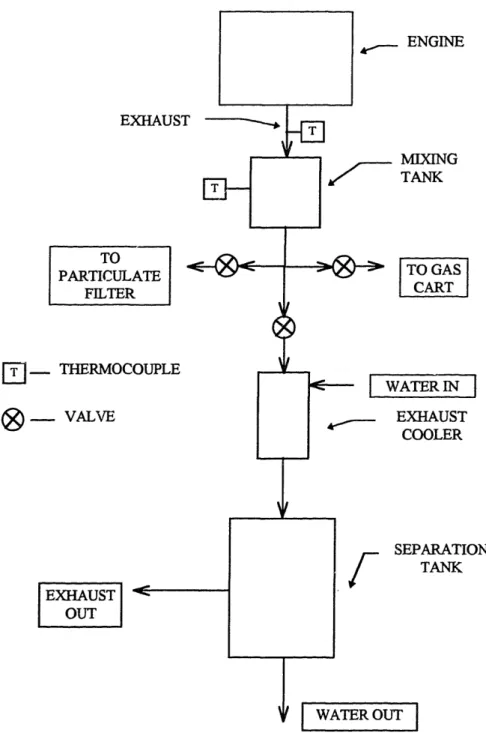
The exhaust system was set up in accordance to the study done by Laurence [2].

It included a "marine" style exhaust system with aqueous injection to cool the exhaust.

This exhaust system was placed well downstream of the oil consumption sampling location

to not effect the oil consumption results. Beyond the aqueous injection apparatus the

exhaust gases were separated in a mixing tank and exhausted into the test cell exhaust trench. The exhaust system also was fitted with a BG- 1 Micro Dilution Tunnel for the

availability of particulate measurement. Figure 2-1 below shows the "marine" type

TO PARTICULE FILTER

I

THERMOC

_

VALVE

Figure 2-1 Exhaust System

The engine was also equipped with the capability to isolate the overhead valve

train oil with that of the engine sump. This was easily accomplished due to the engine's

external stainless lines supplying oil to the overhead valve system. The engine test bed

was modified with the addition of a 1/3 horsepower motor connected to a 0.5 gallon per

minute positive displacement pump. Beyond the pump, a relief valve was installed and set

to 50 psig. An oil cooler was also installed to control the temperature of the valve oil.

Figure 2-2 below shows the details of the external overhead valve oil system.

1/3 HP 1750 RPM 120 VAC MOTOR TCH JRN PLASTIC 1/2 GPM TUBING SPUR GEAR PUMP \ 10 MICRON FILTER

Figure 2-2 Valve Oil System

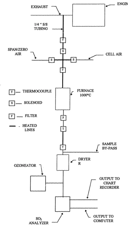
2.2 Oil Consumption Apparatus

The oil consumption of the diesel engine was measured with a pyrofluorescence

sulfuir dioxide testing apparatus developed by Cummins Engine Company, Inc. Figure 2-3

shows the schematic of the instrumentation installation.

EX U ENGINE 1/4 " S/S TUBING FURNACE 1000C DRYER R S02 ANALYZER CELL AIR AMPLE Y-PASS TPUT TO CHART CORDER OUTPUT TO COMPUTER

Figure 2-3 OC Sampling System

The general principal of the system was to trace the sulfur in the oil through the

combustion process and into the exhaust stream. This was accomplished by using a zero

3 -

SOL

[- -

FIL

sulfur diesel fuel and with lubrication oils containing sulfur. By analyzing the sulfur content in the exhaust, the oil consumption could be obtained.

The sampling line was placed in the exhaust manifold near the engine head. The

sample exhaust gas went through heated lines to maintain a high exhaust temperature into

a group of solenoid valves controlling whether the exhaust, span gas, zero gas, or ambient

test cell air would pass through the system. Next the sample passed into a furnace which

operated at 1000°C. Inside the furnace, a quartz combustion tube completed the

oxidation of the unburned fuel and oil. Upon exiting the furnace, the sample was filtered

with a 60 micron filter. This extracted the remaining particulate out of the sample. It then

passed through two heated lines into a membrane dryer which removed the 3-12% water

in the exhaust directly from the vapor phase without condensing the moisture first. The

sample was then mixed with ozone to oxidize the NO to NO

. Finally, the sample's sulfur

dioxide concentration was measured in molar concentration in a pulsed fluorescent

ambient SO

detector. This concentration reading had linear dc voltage outputs which

were tied into a chart recorder and a computer data acquisition system.

The outputs were real-time measurements of the sulfur dioxide concentration

which was directly related to the OC in the engine. The details of the conversion is

discussed in Chapter 4. A chart recorder recorded the results instantaneously during

testing. Its speed was set at 30 cm/hr. This gave visual results while the engine was

operating.

The output of the sulfur dioxide and several other engine operational variables

were recorded directly on a computer data acquisition system. This systein included four

dc voltage outputs from the engine testing cell. These included; air flow, fuel flow, torque, and sulfur dioxide voltage outputs. These signals were input into a computer data

acquisition system using a software system, Global Lab. The data collection was then

saved to a disk in order to make the appropriate conversions in the actual data analysis.

A laboratory manual [13], has been prepared for this work that contains a more

complete description of the OC system and operation. Dr. Victor Wong has a copy of this

Chapter 3 EXPERIMENTATION

3.1 General Overview Of The Testing Procedure

This chapter presents the testing procedure for the oil consumption data. The

actual testing was categorized into three matrices, A, B, and C. All three matrices used zero sulfur diesel and oil containing sulfur. The A matrix was accomplished using a standard oil control ring tension. Matrix B was completed with a lower tensioned oil

control ring. The A and B Matrices had only ring-pack derived oil consumption. Matrices

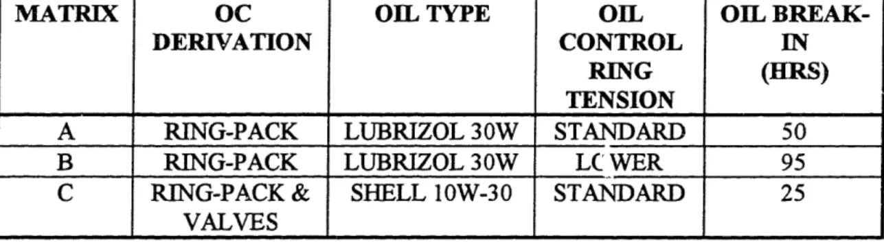
A and B were completed using high sulfur oil, while Matrix C had oil at a normal level of sulfur content. A summary of all three test matrices is given below in Table 3-1.

Table 3-1 Overview of Testing

The table shows the order in which testing was completed and several of the

variables in the testing. Matrix A and most of Matrix B was completed in conjunction

with particulate testing completed by Eric Ford [14]. The engine itself was overhauled

twice during the testing in order to change out the oil control ring. During these periods

the engine was re-assembled as close to the original configuration as possible. The one

exception was with respect to the hydrocarbon build-up on the cylinder liner. These

deposits had to be dissolved with acetone to facilitate the piston assembly removal. Each

of the testing variables will be covered in more detail in Sections 3.2 through 3.4.

LATRIX

OC

OIL TYPE

OIL

OIL

BREAK-DERIVATION

CONTROL

IN

RING

(HRS)

TENSION

A

RING-PACK

LUBRIZOL 30W

STANDARD

50

B

RING-PACK

LUBRIZOL 30W

LC WER

95

C

RING-PACK &

SHELL 10W-30

STANDARD

25

3.2 Testing Procedure For The Standard Oil Control Ring Tension

3.21 Test Matrix A

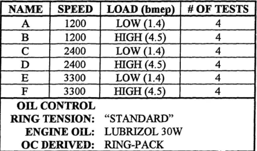
Table 3-2 below shows the details of Matrix A.

NAME

SPEED

LOAD (bmep)

# OF TESTS

A

1200

LOW (1.4)

4

B

1200

HIGH (4.5)

4

D

2400

HIGH (4.5)

4

E

3300

LOW (1.4)

4

F

3300

HIGH (4.5)

4

OIL CONTROL

RING TENSION:

ENGINE OIL:

OC DERIVED:

"STANDARD"

LUBRIZOL 30W

RING-PACK

Table 3-2 Test Matrix A

This matrix included three different speeds, two different loads, and four separate tests for

each load and speed resulting in a total of 24 tests. A low sulfur oil was used for the

overhead valve lubrication and a high sulfur oil was used to lubricate the crankshaft and

piston assemblies. Thas was done to analyze the OC derived mostly from the ring-pack.

The details of the variables can be found in Section 3.23.

3.22 Procedure

In order to ensure repeatable results, the oil was first "broken-in" for 50 hours.

This was to ensure that the oil volatility and viscosity levels were at a steady-state level.

After the initial break-in period, testing followed with up to 6 tests completed in a single

day.

A typical day of testing was started first with the OC system purging and

calibration. A dry zero sulfur gas was input into the system for approximately 45 minutes

zeroing, a standard span gas was sent through the sulfur dioxide detector to establish a

span setting. The span setting was adjustable via a span manual pot and also by a photo-multiplier setting in the sulfur dioxide detector housing. The span setting was then stabilized according to the manufacturer's specifications for a minimum of 6 minutes.

During this time, the linear chart recorder setting and the voltage output to the computer

were logged in a data sheet contained in Appendix A, Figure A-1.

After the initial calibration procedure, the engine was started and warmed up at

idle, 1200 rpm, for approximately 10 minutes. After engine warm-up, the engine was run at the maximum speed and load, 3300 rpm-4.5 bmep, and the oil consumption sample line was opened. This was done in order to burn any residual fuel and oil in the exhaust lines

and to allow the oil consumption apparatus time to "settle out". This period was

approximately 30 minutes. After this initial procedure, the testing was started.

Each day the first test point was Condition F, the maximum speed and load. Each

test point was approximately 45 minutes in duration and included data collection for both

the oil consumption data mentioned in this study and also data for a simultaneous study by

Eric Ford for particulate rate, emissions, and aqueous injection data. The following list

describes the procedure for a typical test:

Time: 0 Minutes: Steady-state engine speed and load obtained. Time: 10 Minutes: Particulate samples taken for 2-5 minute duration. Time: 20 Minutes: Oil consumption computer data acquisition started,

engine control information recorded, and aqueous injection water

samples taken.

Time: 30 Minutes: Exhaust emissions recorded for both before and after

aqueous injection.

Time: 40-50 Minutes: End of test, change load and speed.

The first ten minutes was used for the engine to reach steady-state operation. The

temperatures described in section 2.1 were watched during this time. Most of the

temperatures of the engine reached a steady reading within 5 minutes with the exception

of the oil temperatures. The temperature of the oil out of the engine sump and the oil out

the oil pump took from 5-15 minutes to reach a steady temperature.

At the ten minute point, the particulate sampling was completed. This involved a

and then took an exhaust sample for between 2-4 minutes. At the lower speeds, the

engine load decreased during the filter purging of the particulate testing system due to an

increase in back pressure. This did not ultimately affect the filter or subsequent OC

testing.

After 20 minutes the oil consumption data collection was started using the

computer data acquisition system described in Chapter 2. The data acquisition lasted for

10 minutes with data collected from the four channels with a frequency of 0.2 samples per second, or a sample collection every 5 seconds. Simultaneously, engine temperatures, etc. were recorded onto a data sheet contained in Appendix A, Figure A-2.

At the 30 minute mark, the OC computer data was output to a disk and the

exhaust emissions were recorded.

This same procedure was completed for all the tests in Matrix A and the chart

recorder was on throughout each day of testing. To facilitate the testing and to make the

steady-state transition time minimal, the following order of testing was followed; F, E, B,

A, D, C. Also, after each low load test, the engine was run for 5 minutes at the maximum

speed and load. At the end of the day of testing, the calibration procedure was repeated in

order to ensure accurate results throughout the day.

3.23 Matrix A Engine Specifics, Controls, and Variables

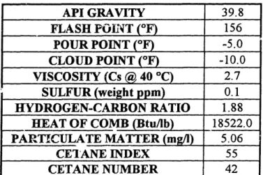
During the testing, the engine was run with a ultra low sulfur diesel so that the fuel

would not contribute to the overall sulfur dioxide concentration. Table 3-3 below gives a summary of the diesel fuel characteristics.

API GRAVITY 39.8

FLASH POINT (F)

156

@

SULFUR (weight ppm)

0.1

HYDROGEN-CARBON RATIO

1.88

HEAT OF COMB (Btu/lb)

18522.0

PARTICULATE MATTER (mg/l)

5.06

CEIANE INDEX 55

CETANE NUMBER 42

Table 3-3 Diesel Fuel Characteristics

Throughout this matrix, the overhead valve oil system was separated from the main oil system. The characteristics of both oils are summarized in Table 3-4.

Table 3-4 Oil Characteristics

The ring-pack configuration was the standard as per the manufacturer's

specifications. The first ring or compression ring was chrome plated and slightly rounded in shape. The second ring or scraper ring was beveled. The third ring or oil control ring

was chrome plated with two rails and a separate coil spring for tension control. Although

the ring characteristics were not measured directly, Table 3-5 below shows the

manufacturer's specifications.

LUBRICATION BRAND TYPE SULFUR CONTENT

(% by weight)

VALVE SHELL FIRE AND SAE 10W-30 0.279

ICE ALL SEASON

MAIN ENGINE

LUBRIZOL HIGH

SAE 30W

1.27

RING DIAMETER (mm) COLD GAP (mm) TENSION (N)

COMPRESSION 80.25 0.43 9.3

SCRAPER 80.25 0.43 8.2

OIL CONTROL 80.25 0.51 53.8

Table 3-5 Piston Ring-Pack Characteristics

The importance of controls cannot be overlooked. The most important control feature was the repeatability of the engine temperatures described in section 2.1. Of these, the oil temperatures were continually monitored to ensure the engine had reached a

steady-state operation. However, there was no external heating or cooling of the oil to

specific pre-set temperatures.

Matrix A had two variables, speed and load. The brake mean effective pressure

(bmep) was kept constant throughout the speed range of the testing. Table 3-6 below

shows the target load, bmep, fuel flow rate, and exhaust temperature for the testing.

SPEED

ENGINE

BMEP

FUEL FLOW

INJECTION

EXHAUST

(rpm)

LOAD

(bar)

RATE

TIMING

TEMP

(cc/min) °BTDC (C) 1200 LOW 1.4 7.0 9 235 1200 HIGH 4.5 15.3 9 445 2400 LOW 1.4 14.8 14 280 2400 HIGH 4.5 28.5 14 480 3300 LOW 1.4 24.3 15.5 375 3300 HIGH 4.5 46.1 15.5 610

Table 3-6 Matrix A Variable Specifics

3.3 Testing Procedure For The Less Tensioned Oil Control Ring

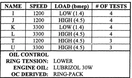
3.31 Test Matrix B

Table 3-7 Test Matrix

This matrix was done with similar parameters to that of Matrix A. Again, the overhead valve system was separated. The major change was that a modified oil control ring with 45 % less tension was substituted for the original in the ring-pack.

3.32 Procedure

The procedure for tests I through L were done as per the procedure addressed in

Section 3.22. The tests, T and U, were done to study the long term variability of the data

and were not completed in conjunction with particulate or emission testing. Their

procedures are addressed below.

For these tests, the calibration procedures were repeated as before. Each test had

a duration of 60 minutes outlined as follows:

Time: 0 Minutes: Steady-state engine speed and load obtained.

Time: 15 Minutes: Oil consumption computer data acquisition started. Time: 30 Minutes: Engine control information recorded.

Time: 60 Minutes: End of test, change load and speed.

The first fifteen minutes was used for the engine to reach steady-state operation.

The temperatures described in Section 2.1 were watched during this time. Most of the

temperatures of the engine reached a steady reading within 5 minutes with the exception

NAME SPEED LOAD (bmep) # OF TESTS

I 1200 LOW (1.4) 4

J

1200

HIGH (4.5)

4

U_

3300

HIGH (4.5)

3

OIL CONTROL

RING TENSION: LOWER

ENGINE OIL: LUBRIZOL 30W

OC DERIVED: RING-PACK

of the oil temperatures. The temperature of the oil out of the engine sump and the oil out

the oil pump took from 5-15 minutes to reach a steady temperature.

After 15 minutes the oil consumption data collection was started using a computer

data acquisition system described in Chapter 2. The data acquisition lasted for 45 minutes

with data collected from the four channels with a frequency of 0.2 samples per second, or

a sample collection every 5 seconds.

At the 30 minute point, the engine control parameters of speed, load, etc. were recorded onto a data sheet contained in Appendix A, Figure A-2.

At the 60 minute mark, the OC computer data was output to a disk and the exhaust emissions were recorded.

This same procedure was completed for all tests T and U in Matrix B and the chart

recorder was on throughout each day of testing. At the end of the day of testing, the

calibration procedure was repeated in order to ensure accurate results throughout the day.

3.33 Matrix B Engine Specifics, Controls, and Variables

All of the engine specifics, controls, and variables were the same as Matrix A with the exception of the ring-pack oil control ring tension. A new oil control ring was

installed with a lower tension as shown in Table 3-8.

RING

DIAMETER (mm)" COLD GAP (mm)

TENSION (N)

OIL CONTROL 80.25 0.51 30.3

Table 3-8 Modified Oil Control Ring Characteristics

3.4 Testing Procedure For The Commercially Available Oil

3.41 Test Matrix C

Table 3-9 Test Matrix C

This matrix was completed with the engine oil system in its standard configuration with the sump oil also being distributed to the overhead valves.

3.42 Procedure

The procedure for all of these tests were the same as the procedure from Matrix B

for the tests, T and U. Prior to the testing, the engine was run at the maximum speed and load for 25 hours in order to break-in the oil prior to testing.

3.43 Matrix C Engine Specifics, Controls, and Variables

All of the engine specifics, controls, and variables were the same as Matrix A with the exception of the engine oil. Instead of using a high sulfur oil, a commercially available

oil was used. The oil was a commercially available Shell oil. Its characteristics are listed

below in Table 3-10.

Table 3-10 Commercially Available Oil Characteristics

NAME

SPEED LOAD (bmep)

# OF TESTS

REGA 1200 LOW (1.4) 4

REGB 1200 HIGH (4.5) 4

REGF

3300

HIGH (4.5)

4

OIL CONTROL

RING TENSION: "STANDARD"

ENGINE OIL: SHELL 10W-30

OC DERIVED: RING-PACK & VALVES

LUBRICATION

BRAND

TYPE

SULFUR CONTENT

(% by weight)

ENTIRE SHELL SAE 10W-30 0.8

Chapter 4 THEORY

4.1 General

The output of the analyzer is in terms of sulfur dioxide volumetric concentration in

the exhaust. This section analyzes how to convert the sulfur dioxide concentrations into

useable oil consumption results.

The first important factor in the analysis of the data is that the concentration of the

sulfur dioxide is detected in a dry exhaust gas stream. The water content of the wet

exhaust must be known in order to account for this lost water. By using dry gaseous

emissions, Heywood [15], offers an equation to determine the molar concentration of

water in the exhaust derived from the combustion process. Equation 4-1 describes this

equation.

H20combmol =

0.5y CO2m!

COm.

(4-1)

COmo]

3.8(CO2mo,) + 1

where:

H20combmol = water in exhaust due to combustion (% molar)

COmo

= carbon monoxide concentration in exhaust (% molar)

y = relative hydrogen to carbon ratio

Now, given a fuel molecule comprised of CaHb and the fuel and air flow rates and

(va )(Pa)

(4-2)

34.56(4 + y)

12.011 + 1.008y

where:

va =

volumetric air flow

Vf = volumetric fuel flow rate (cc/min)

Pa = density of air (g/m3)

pf =

density of fuel (g/cc)

y = relative hydrogen to carbon ratio

Using this relative air to fuel ratio, Laurence [2], gives the following equation to

calculate the molecular weight of the exhaust.

MW

6a+18+ 16([2(a

+)-(2a +

))+

106.25A(a+

4)

MW=

a+

0.5([2(a +

-

(2a

+

)

+

3.773(a +

)

where:

MAWCh = molecular weight of exhaust (g/g-mole) a = number of carbon atoms per fuel molecule b = number of hydrogen atoms per fUel molecule

Next, usihig the exhaust molecular weight, Equation 4-1 can be converted to

weight basis using the Equation 4-4.

H

where:

H20 ,mbwt

= water in exhaust due to combustion (% by weight)

With a known relative humidity and temperature, psychrometric charts can be used

to find the weight fraction of water in the air. This can ultimately lead to the water

content in the air. Using this percentage and that of the combustion derived water, the

total water content of the exhaust can be found.

H20air (H2Ow)(PaVa)(100)

(45)

EXHtot,

H

H

+ H20air

(4-6)

where:

H

Owf

= fraction of water in the air

EXHtot

= exhaust flow rate (g/hr)

H2Oar = water in the air (% by weight)

H2 0exh =

total water in exhaust (% by weight)

Using an output voltage from the detector for a given test, the voltage and

concentration of sulfur dioxide in a span gas, the total sulfur dioxide flow rate in the dry

exhaust can be determined.

S.b

(SAMPv,):t

(EXH,)(PANPP)

()

S = ,S-o

J

(4-7)

ah SPANTL 2 x 106 g

where:

SPANpro

= span gas sulfur dioxide concentration (ppm by weight)

SPANvolt

= output voltage of detector using span gas (volt)

SAMPVooI

:

detector output of current test (volt)

Sexh = sulfur dioxide exhaust flow rate (g/hr)

From this sulfur dioxide flow rate, the oil consumption can be found using the

equation below. This equation includes the correction of the fuel sulfur content and also

the ambient air concentration. It also corrects for the water concentration in the exhaust

OC=s

[(pf)(Vf)(FUEL)

I

(AIRo,,) ()(V

)(PAN

)lY

)')i1]

L x 106 (SPANVO,) 2

x

(4-8)

where:

FUE,Lp, = sulfur content in fuel (ppm by weight)

AIRvolt = output voltage of detector using cell air (volt) LUBE, = sulfur content of lube oil (% by weight)

OC = oil consumption of engine (g/hr)

4.2 Matrix Application

The equations above were used to etermine both the average oil consumption and also the instantaneous oil consumption traces. The following shows how these equations were applied to the testing.

After testing, the computer outputs of sulfur dioxide voltage, air flow, fuel flow, and torque as well as gaseous emissions and calibration data were transferred into a spreadsheet. Using the average values of fuel flow and air flow, the water content of the

exhaust was computed using Equations 4-1 through 4-6. Using this value and each

sample's real-time voltage, the sulfur flow rate in the exhaust was determined using

Equation 4-7. Then, using Equation 4-8, the instantaneous oil consumption trace values

were determined. Averaging these values as well as the torque outputs, each test's average OC and SOC were determined.

Chapter 5 RESULTS AND ANALYSIS

5.1 Results For The Standard Oil Control Ring

5.11 Matrix A Steady-State Oil Consumption

Figure B-1 in Appendix B shows the steady-state results that were calculated in

accordance to the equations in Chapter 4. Figures B-2 and B-3 show the OC results in

graphic form. Table 5-1 below shows the specific oil consumption (SOC), time averaged

over the 10 minutes testing cycle, for each of the four tests, their sample standard

deviations, and their coefficients of variation.

CONDITION

AVERAGE

SAMPLE

COEFFICIENT

SOC

STANDARD

OF

A-1200 LOW

0.220

0.012

5.61

C-2400 LOW

1.147

0.224

19.51

E-3300 LOW

0.752

0.095

12.68

Table 5-1 Summary of Matrix A Steady-State SOC Results

The above results do not include those of Condition D from the original test

matrix. At this operating point, 2400 rpm-4.5bmep, the oil consumption was higher than

that which could be measured by the oil consumption apparatus. The SOC at this point

appears to be higher than approximately 1.34 g/kw-hr. Condition C also had relatively high SOC values with high variability. This suggests that there may be a dynamic effect in

the ring-pack at the 2400 rpm speed that causes higher SOC.

The data shows that at Conditions A and F, there is excellent repeatability in SOC from day to day testing. The trends show that the SOC at a given speed is lower at the higher load, which is what would be expected. Also, the trends indicate that the SOC is increasing from low speed to a high speed with a peak in SOC at the mid speed range

5.12 Variability Of Matrix A During Steady-State Operation

Appendix C shows graphs of the computer real-time results of each operating

condition over the ten minute testing cycle. The OC values were normalized with respect

to the average OC values of all four tests. This normalization makes it easier to compare

different conditions and matrice.

The results show similar trends to those found in Section 5.11 above. For the

most part, the graphs all show small variability patterns, deviation less than 10 percent of

each test's mean OC value. The small "peaks and valleys" during many of the tests may represent small fuel and load variations that are frequently observed in single cylinder engines. Conditions A, E, and F show this pattern with no large OC variations in each test or from test to test. Conditions B and C show some larger variability in the average OC

values from test to test.

Figure C-2 shows the results of Condition B. There is a definite change in OC from test to test, and this OC level is not a function of the actual load on the engine. Test B4 has a relatively high OC, but with the lowest average load for the testing duration. Test B 1 shows a OC trace with larger than 10 percent variability in OC. The periods of these are between 1 and 3 minutes in duration. Again this may be a dynamic effect in the

ring-pack.

Figure C-3 shows the results of Condition C. This data is also variable from test

to test and is not a function of the actual average load. Another interesting result can be

seen in Test C3. Near the end of the test, the OC increases by 50 percent. Studying the

linear chart recording of this test, Figure C-6 in Appendix C, shows interesting trends.

When the engine was first run at Condition C, an OC "plateau," constant OC period, occurred. This constant OC continued for approximately 12 minutes, then increased by 25 percent to a plateau lasting 15 minutes during which time the data for Test C3 was

recorded. This non-periodic phenomenon is not easily explainable. While these plateaus were occurring, the engine load, fuel flow, etc. did not noticeably change.

The chart recording of Test C2, Figure C-7 in Appendix C, also shows similar type

results. At the beginning of Test C2, the OC was at a constant "plateau" for about 30

minutes during which the C2 results were recorded. At this point the OC instantly

increased by 100 % to a plateau lasting 15 minutes, at which time the OC trace instantly

changed back to the original OC level.

5.2 Results For The Less Tensioned Oil Control Ring

5.21 Matrix B Steady-State Oil Consumption

Figure D-1 in Appendix D shows the steady-state results that were calculated in

accordance to the equations in Chapter 4. Figures D-2 through D-5 show the OC and

SOC results in graphic form. Table 5-1 below shows the SOC results, time averaged over

the 10 minutes testing cycle, for each of the four tests, their sample standard deviations,

and their coefficients of variation.

CONDITION

AVERAGE

SAMPLE

COEFFICIENT

SOC

STANDARD

OF

kw-hr)

I-1200 LOW

0.183

0.030

16.29

J-1200 HIGH

0.195

0.050

25.96

L-3300 HIGH

0.718

0.149

20.71

T-1200 HIGH

0.166

0.038

22.89

U-3300 HIGH

0.678

0.131

19.32

Table 5-2 Summary of Matrix B Steady-State SOC Results

The results do not include data from Condition K, 3300 low load, because during

this condition, the engine operation was unsteady. The load varied as much as 75 percent

and the engine sounded as if poor combustion was taking place. Also, the first set of tests

were not recorded due to problems with the OC apparatus.

These results show a large variability in the average SOC values as shown by the high coefficients of variation. Unlike the results from Matrix A, Conditions I and L, 3300

rpm-4.5 bmep, even show large deviations from test to test. This is further analyzed in

Section 5.22.

5.22 Variability Of Matrix B During Steady-State Operation

This matrix included both the original ten minute OC tests as well as longer 45 minute duration tests, Conditions T and U. These results show high variability and

cyclical spikes of OC. Appendix E contains the graphs of the real-time OC results with

normalized OC values that were normalized with respect to the average OC values of all

four tests.

Conditions J3 and J4 in Figure E-2 both contain very similar plots of OC. In both cases there is a "spike" in the OC plots during the middle of the tests with about 50%

hig-er instantaneous OC. Both spikes occur at approximately 24 minutes after the tests

were started. Test J3 also had two smaller spikes one 2 minutes prior to the large spike and the other 4 minutes after the large spike.

Condition L also shows patterns of unstable OC during the 10 minute testing

period not seen in Matrix A. Test L2, Figure E-3, shows the same "plateau" effect as was found during Matrix A, Condition C. This plateau shows an OC of about 58 % higher

than the steady-state period before or after with a duration of about 7 minutes. Condition

L5 shows a spike of oil consumption that was unmeasurable but greater than an OC of 6

g/hr.

Because of the large variability of data in Tests I, J, and L, longer term Tests, T

and U, were completed. These tests were completed as per Section 3.32. Condition T,

Figure E-4, shows a large spiking phenomenon during the 45 minute testing. Condition

T3 shows a large spike and a smaller spike with a 13 minute period. Condition T2 shows two small spikes with a 4 minute period.

Figure E-5 shows very interesting results. Test U2 shows two spikes during the testing with an instantaneous OC increase of 75% and 35%, respectively. These spikes are separated by approximately 20 minutes. Test U3 shows some interesting spikes with a

6 g/hr in magnitude. Just prior to the testing another large spike also occurred. The

period between the first two is about 14 minutes and the second about 16 minutes in duration. Both of these spikes led to a very cyclical pattern with several smaller spikes following the large spikes.

Overall, this Matrix B shows much more variability in steady-state OC than Matrix A. The spikes and plateaus may be a phenomena explained by the studies conducted by Hiruma et al., and by Schneider et al. [16], [17]. They suggest that ring dynamics such as ring lift off, rotation, and ring twist may cause significant changes in OC. The

instantaneous spikes may be caused by a slow ring rotation phenomena in the ring-pack.

When the ring gaps line up, or the top ring lifts off its the piston groove, a relatively large

amount of oil may be transported into the cylinder by reverse blow-by. The OC plateaus may be caused by the ring position becoming steady at another position. This temporary position may be ultimately effected by the transport of oil in the ring-pack. The transport of oil may accumulate in the second land and then suddenly when reaching a critical point, cause the ring positions to change and hence a different OC.

5.3 Results For The Commercially Available Oil

5.31 Matrix C Steady-State Oil Consumption

Figure F-1 in Appendix F shows the steady-state results which were calculated in

accordance to the equations in Chapter 4. Figures F-2 and F-3 show the OC and SOC

results in graphic form. Table 5-3 below shows SOC values, time averaged over 45 minutes for each condition, their sample standard deviations, and their coefficients of

CONDITION

AVERAGE

SAMPLE

COEFFICIENT

(g/kw-hr)

DEVIATION

VARIATION

REGA-1200 LOW

0.376

0.097

25.80

REGF-3300 HIGH

0.769

0.022

2.86

Table 5-3 Summary of Matrix C Steady-State SOC Results

The coefficients of variation show excellent repeatability for the Condition REGF.

The other two conditions show larger repeatability errors which may be due to variability discussed in Section 5.32.

5.32 Variability Of Matrix C During Steady-State Operation

Figures G-1 through G-3 in Appendix G show the steady-state OC results for Matrix C. These graphs show different variations in the real-time OC than those found in

Matrix A or B. With the exception of REGB4, Figure G-2, no OC spiking occurred. At

the same time though, there was more variability in each test as well as between tests for conditions REGB and REGA than those same conditions in Matrix A. This may be due to the OC of this matrix was contributed by both the valves and the ring-pack. This

difference may be in the variability of the valve real-time OC. All three figures show a

trend that by the end of the testing period, the OC levels of the tests tend to end with very

close values. This may show that the engine reached a final steady-state OC period at the end of 1 hour of operation at a given speed and load, potentially caused by an usteady valve OC.

5.4 Comparison Of Matrices A, B, C

5.41 Ring-Pack OC Evaluation

Figure H- 1 of Appendix H shows a comparison of Matrix A results to that of the

entire engine SOC results that were conducted prior to this testing. By knowing the entire

engine SOC and that of the ring-pack only, the valve oil contribution can be calculated

using the oil consumption values, the sulfur content of the oils, and simultaneous

equations. Table 5-4 below summarizes the comparison.

CONDITION

VALVE OIL

VALVE OIL

CONTRIBUTION TO

CONTRIBUTION TO

ENTIRE SOC (%) MATRIX A (%)

1200 Rpm Low Load

56

22

1200 Rpm High Load

47

17

3300 Rpm High Load

42

14

Table 5-4 Valve Oil Contribution

The results show that in this engine, the valve oil contribution is relatively high. It

also shows that there is a small contribution of OC from the valves in Matrices A and B.

5.42 Effects Of The Less Tensioned Oil Control Ring

Figure H-2 shows the comparison of the average SOC results for matrix A to that

of Matrix B. The results are compared in Table 5-5.

CONDITION

CHANGE IN SOC FROM STANDARD

TO LESS TENSIONED OIL CONTROL

RING (%)

1200 Rpm Low Load - 16.8

1200 Rpm High Load

- 2.0

3300 Rpm High Load

+ 63.2

This table shows an interesting result. By decreasing the oil control ring tension by approximately 45%, the SOC values increased at 3300 rpm and decrease at 1200 rpm.

The expected result would be for the SOC to increase over the entire speed and load range

due to lower tensioned oil control ring causing higher oil film thickness' on the liner. One

factor that they may have contributed to these results is that the engine was rebuilt after

Matrix A in order to change out the oil control ring. Deposits on the liner had to be

removed in order to facilitate the piston removal. This may have ultimately affected the

low speed results.

5.43 Comparison Of Commercially Available Oil To High Sulfur Oil

Figure H-3 shows the graphical representation of the regular oil results of Matrix

C to that of the high sulfur results of the entire engine SOC prior to the testing. Table 5-6

shows the comparison.

CONDITION

DIFFERENCE IN SOC RESULTS

USING COMMERCIALLY

AVAILABLE

OIL (%)

1200 Rpm Low Load

2.6

3300 Rpm High Load

15.2

Table 5-6 Matrix C to High Sulfur Oil SOC Comparison

These percentage differences are small comparing these two operating conditions.

This suggests that this oil may be suitable for testing at these two operating conditions. A

source of error in comparing these two tests may be in the oil used. The "regular" oil was