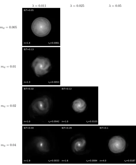
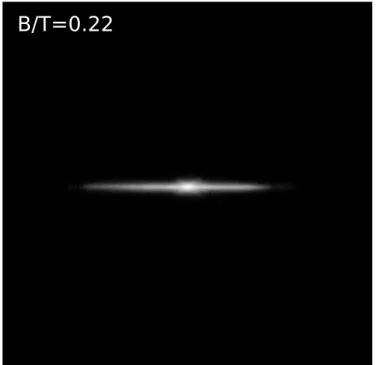
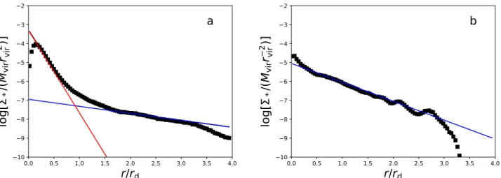
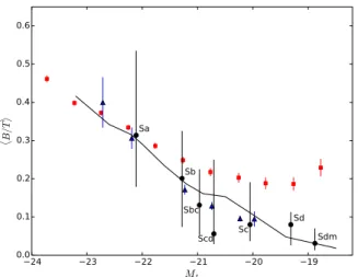
Bulge formation through disc instability
Texte intégral
Figure
Documents relatifs
Le but de l’exercice est de « construire » un espace vectoriel normé de dimension infinie, de le munir de deux normes non équivalentes mais qui font de cet evn un Banach. Soit (E , k
In this work we prove the nonlinear instability of inhomogeneous steady states solutions to the Hamiltonian Mean Field (HMF) model.. We first study the linear instability of this
[r]
– 3 ﺎﻤ ﺡﺎﺒﺴﻟﺍ ﻥﻴﺒ ﺱﻤﻼﺘﻟﺍ ﺔﻁﻘﻨ ﺕﺎﻴﺜﺍﺩﺤﺇ ﻲﻫ ﺀﺎﻤﻟﺍﻭ.. – 4 ﺀﺎﻤﻟﺍ ﺢﻁﺴ ﻪﺘﺴﻤﻼﻤ
The corresponding transition metal complexes have shown impressive reactivity for alcohol dehydrogenation and selective formation of acetals or esters.14 Observing the efficiency
On suppose qu’il existe une fonction int´ egrable f telle que 1/f soit ´ egalement int´ egrable.. Que peut-on dire de la mesure
Les fonctions sont intégrables car elles sont majorées en valeur absolue par √ 1 t e −t qui est intégrable d'après la question précédente.. Il est clair que u est paire et v
Chacun de ces (petits) intervalles ne peut contenir qu'au plus un élément de G.. Par conséquent, l'intersection de G avec un tel intervalle (borné quelconque) est vide
