HAL Id: hal-00328500
https://hal.archives-ouvertes.fr/hal-00328500
Submitted on 7 May 2007
HAL is a multi-disciplinary open access
archive for the deposit and dissemination of
sci-entific research documents, whether they are
pub-lished or not. The documents may come from
teaching and research institutions in France or
abroad, or from public or private research centers.
L’archive ouverte pluridisciplinaire HAL, est
destinée au dépôt et à la diffusion de documents
scientifiques de niveau recherche, publiés ou non,
émanant des établissements d’enseignement et de
recherche français ou étrangers, des laboratoires
publics ou privés.
GISS modelE study
J. Hansen, M. Sato, R. Ruedy, P. Kharecha, A. Lacis, R. Miller, L. Nazarenko,
K. Lo, G. A. Schmidt, G. Russell, et al.
To cite this version:
J. Hansen, M. Sato, R. Ruedy, P. Kharecha, A. Lacis, et al.. Dangerous human-made interference with
climate: a GISS modelE study. Atmospheric Chemistry and Physics, European Geosciences Union,
2007, 7 (9), pp.2312. �10.1007/s00382-007-0255-8�. �hal-00328500�
www.atmos-chem-phys.net/7/2287/2007/ © Author(s) 2007. This work is licensed under a Creative Commons License.
Chemistry
and Physics
Dangerous human-made interference with climate: a GISS modelE
study
J. Hansen1,2, M. Sato2, R. Ruedy3, P. Kharecha2, A. Lacis1,4, R. Miller1,5, L. Nazarenko2, K. Lo3, G. A. Schmidt1,4, G. Russell1, I. Aleinov2, S. Bauer2, E. Baum6, B. Cairns5, V. Canuto1, M. Chandler2, Y. Cheng3, A. Cohen6, A. Del Genio1,4, G. Faluvegi2, E. Fleming7, A. Friend8, T. Hall1,5, C. Jackman7, J. Jonas2, M. Kelley8, N. Y. Kiang1, D. Koch2,9, G. Labow7, J. Lerner2, S. Menon10, T. Novakov10, V. Oinas3, Ja. Perlwitz5, Ju. Perlwitz2, D. Rind1,4, A. Romanou1,4, R. Schmunk3, D. Shindell1,4, P. Stone11, S. Sun1,11, D. Streets12, N. Tausnev3, D. Thresher4, N. Unger2, M. Yao3, and S. Zhang2
1NASA Goddard Institute for Space Studies, New York, NY, USA 2Columbia University Earth Institute, New York, NY, USA 3Sigma Space Partners LLC, New York, NY, USA
4Department of Earth and Environmental Sciences, Columbia University, New York, NY, USA 5Department of Applied Physics and Applied Mathematics, Columbia University, New York, NY, USA 6Clean Air Task Force, Boston, MA, USA
7NASA Goddard Space Flight Center, Greenbelt, MD, USA
8Laboratoire des Sciences du Climat et de l’Environnement, Orme des Merisiers, Gif-sur-Yvette Cedex, France 9Department of Geology, Yale University, New Haven, CT, USA
10Lawrence Berkeley National Laboratory, Berkeley, CA, USA 11Massachusetts Institute of Technology, Cambridge, MA, USA 12Argonne National Laboratory, Argonne, IL, USA
Received: 23 October 2006 – Published in Atmos. Chem. Phys. Discuss.: 5 December 2006 Revised: 29 March 2007 – Accepted: 15 April 2007 – Published: 7 May 2007
Abstract. We investigate the issue of “dangerous
human-made interference with climate” using simulations with GISS modelE driven by measured or estimated forcings for 1880– 2003 and extended to 2100 for IPCC greenhouse gas scenar-ios as well as the “alternative” scenario of Hansen and Sato (2004). Identification of “dangerous” effects is partly sub-jective, but we find evidence that added global warming of more than 1◦C above the level in 2000 has effects that may be highly disruptive. The alternative scenario, with peak added forcing ∼1.5 W/m2 in 2100, keeps further global warming under 1◦C if climate sensitivity is ∼3◦C or less for dou-bled CO2. The alternative scenario keeps mean regional sea-sonal warming within 2σ (standard deviations) of 20th cen-tury variability, but other scenarios yield regional changes of 5–10σ , i.e. mean conditions outside the range of local ex-perience. We conclude that a CO2 level exceeding about 450 ppm is “dangerous”, but reduction of non-CO2forcings can provide modest relief on the CO2 constraint. We dis-cuss three specific sub-global topics: Arctic climate change,
Correspondence to: J. Hansen
(jhansen@giss.nasa.gov)
tropical storm intensification, and ice sheet stability. We sug-gest that Arctic climate change has been driven as much by pollutants (O3, its precursor CH4, and soot) as by CO2, of-fering hope that dual efforts to reduce pollutants and slow CO2growth could minimize Arctic change. Simulated re-cent ocean warming in the region of Atlantic hurricane for-mation is comparable to observations, suggesting that green-house gases (GHGs) may have contributed to a trend toward greater hurricane intensities. Increasing GHGs cause sig-nificant warming in our model in submarine regions of ice shelves and shallow methane hydrates, raising concern about the potential for accelerating sea level rise and future pos-itive feedback from methane release. Growth of non-CO2 forcings has slowed in recent years, but CO2emissions are now surging well above the alternative scenario. Prompt ac-tions to slow CO2emissions and decrease non-CO2forcings are required to achieve the low forcing of the alternative sce-nario.
1 Introduction
The Earth’s atmospheric composition and surface properties are being altered by human activities. Some of the alter-ations are as large or larger than natural atmosphere and surface changes, even compared with natural changes that have occurred over hundreds of thousands of years. There is concern that these human-made alterations could substan-tially alter the Earth’s climate, which has led to the United Nations Framework Convention on Climate Change (United Nations, 1992) with the agreed objective “to achieve stabi-lization of greenhouse gas concentrations in the atmosphere at a level that would prevent dangerous anthropogenic inter-ference with the climate system.”
The Earth’s climate system has great thermal inertia, re-quiring at least several decades to adjust to a change of cli-mate forcing (Hansen et al., 1984). Anthropogenic physical infrastructure giving rise to changes of atmospheric compo-sition, such as power plants and transportation systems, also has a time constant for change of several decades. Thus there is a need to anticipate the nature of anthropogenic climate change and define the level of change constituting danger-ous interference with nature. Simulations with global climate models on the century time scale provide a tool for address-ing that need. Climate models used for simulations of future climate must be tested by means of simulations of past cli-mate change.
We carry out climate simulations using GISS atmospheric modelE documented by Schmidt et al. (2006), hereafter mod-elE (2006). Specifically, we attach the model III version of atmospheric modelE to the computationally efficient ocean model of Russell et al. (1995). This coupled model and its climate sensitivity have been documented by a large set of simulations carried out to investigate the “efficacy” of var-ious climate forcings (Hansen et al., 2005a), hereafter Effi-cacy (2005). We use the same model III here for transient climate simulations for 1880–2100, with a few simulations extended to 2300.
We made calculations for each of ten individual climate forcings for the period 1880–2003, as well as for all forcings acting together. The simulations using all ten forcings were extended into the future using scenarios of atmospheric com-position defined by the Intergovernmental Panel on Climate Change (IPCC, 2001) and two scenarios defined by Hansen and Sato (2004). The simulations for 1880–2003 with indi-vidual forcings are described by Hansen et al. (2007a). Ex-tensive diagnostics and convenient graphics for all of the runs are available at http://data.giss.nasa.gov/modelE/climsim/. Diagnostics for extended runs with all forcings acting at once are also available from the official IPCC repository (http://www-pcmdi.llnl.gov/ipcc/about ipcc.php).
Section 2 defines the climate model and summarizes prin-cipal known deficiencies. Section 3 defines time-dependent climate forcings that we employ. Section 4 examines simu-lated global temperature change and specific regional climate
change issues. Section 5 compares trends of actual climate forcings and those in the scenarios. Section 6 summarizes the relevance of our results to the basic question: is there still time to avoid dangerous human interference with climate? This final section goes one step beyond the usual scientific paper, as it aims to interpret results in terms of policy op-tions and stimulate discussion of the role of scientists in the climate debate.
2 Climate model
2.1 Atmospheric model
The atmospheric model employed here is the 20-layer ver-sion of GISS modelE (2006) with 4◦×5◦horizontal resolu-tion. This resolution is coarse, but use of second-order mo-ments for numerical differencing improves the effective reso-lution for the transport of tracers. The model top is at 0.1 hPa. Minimal drag is applied in the stratosphere, as needed for numerical stability, without gravity wave modeling. Strato-spheric zonal winds and temperature are generally realistic (Fig. 17 in Efficacy, 2005), but the polar lower stratosphere is as much as 5–10◦C too cold in the winter and the model produces sudden stratospheric warmings at only a quarter of the observed frequency. Model capabilities and limitations are described in Efficacy (2005) and modelE (2006). Defi-ciencies are summarized below (Sect. 2.4).
2.2 Ocean representation
In this paper we use the dynamic ocean model of Russell et al. (1995). One merit of this ocean model is its efficiency, as it adds negligible computation time to that for the atmosphere when the ocean horizontal resolution is the same as that for the atmosphere, as is the case here. There are 13 ocean lay-ers of geometrically increasing thickness, four of these in the top 100 m. The ocean model employs the KPP param-eterization for vertical mixing (Large et al., 1994) and the Gent-McWilliams parameterization for eddy-induced tracer transports (Gent et al., 1995; Griffies, 1998). The resulting Russell et al. (1995) ocean model produces a realistic ther-mohaline circulation (Sun and Bleck, 2006), but yields un-realistically weak El Nino-like variability as a result of its coarse resolution.
Interpretation of climate simulations and observed climate change is aided by simulations with the identical atmospheric model attached to alternative ocean representations. We make calculations with the same time-dependent 1880–2003 climate forcings of this paper and same atmospheric model attached to: (1) ocean A, which uses observed sea surface temperature (SST) and sea ice (SI) histories of Rayner et al. (2003); (2) ocean B, the Q-flux ocean (Hansen et al., 1984; Russell et al., 1985), with specified horizontal ocean heat transports inferred from the ocean A control run and diffusive uptake of heat anomalies by the deep ocean; (3) ocean C, the
dynamic ocean model of Russell et al. (1995); (4) ocean D, the Bleck (2002) HYCOM ocean model. Results for ocean A and B are included in Hansen et al. (2007a) and on our (GISS) web site, results for ocean C are in this paper and our web site, and results for ocean D will be presented elsewhere and on our web site.
2.3 Model sensitivity
The model has sensitivity 2.7◦C for doubled CO2when cou-pled to the Q-flux ocean (Efficacy, 2005), but 2.9◦C when coupled to the Russell et al. (1995) dynamical ocean. The slightly higher sensitivity with ocean C became apparent when the model run was extended to 1000 years, as the sea ice contribution to climate change became more important relative to other feedbacks as the high latitude ocean temper-atures approached equilibrium. The 2.9◦C sensitivity
corre-sponds to ∼0.7◦C per W/m2. In the coupled model with the Russell et al. (1995) ocean the response to a constant forcing is such that 50% of the equilibrium response is achieved in
∼25 years, 75% in ∼150 years, and the equilibrium response is approached only after several hundred years. Runs of 1000 years and longer are available on the GISS web site. The model’s climate sensitivity of 2.7–2.9◦C for doubled CO2is well within the empirical range of 3±1◦C for doubled CO2 that has been inferred from paleoclimate and other obser-vational evidence (Hansen et al., 1984, 1993; Hoffert and Covey, 1992; Annan and Hargreaves, 2006).
2.4 Principal model deficiencies
ModelE (2006) compares the atmospheric model climatol-ogy with observations. Model shortcomings include ∼25% regional deficiency of summer stratus cloud cover off the west coast of the continents with resulting excessive absorp-tion of solar radiaabsorp-tion by as much as 50 W/m2, deficiency in absorbed solar radiation and net radiation over other tropical regions by typically 20 W/m2, sea level pressure too high by 4–8 hPa in the winter in the Arctic and 2–4 hPa too low in all seasons in the tropics, ∼20% deficiency of rainfall over the Amazon basin, ∼25% deficiency in summer cloud cover in the western United States and central Asia with a corre-sponding ∼5◦C excessive summer warmth in these regions. In addition to the inaccuracies in the simulated climatology, another shortcoming of the atmospheric model for climate change studies is the absence of a gravity wave representa-tion, as noted above, which may affect the nature of interac-tions between the troposphere and stratosphere. The strato-spheric variability is less than observed, as shown by anal-ysis of the present 20-layer 4◦×5◦ atmospheric model by J. Perlwitz (personal communication). In a 50-year control run Perlwitz finds that the interannual variability of seasonal mean temperature in the stratosphere maximizes in the region of the subpolar jet streams at realistic values, but the model produces only six sudden stratospheric warmings (SSWs) in
50 years, compared with about one every two years in the real world.
The coarse resolution Russell ocean model has realistic overturning rates and inter-ocean transports (Sun and Bleck, 2006), but tropical SST has less east-west contrast than ob-served and the model yields only slight El Nino-like vari-ability (Fig. 17, Efficacy, 2005). Also the Southern Ocean is too well-mixed near Antarctica (Liu et al., 2003), deep wa-ter production in the North Atlantic Ocean does not go deep enough, and some deep-water formation occurs in the Sea of Okhotsk region, probably because of unrealistically small freshwater input there in the model III version of modelE. Global sea ice cover is realistic, but this is achieved with too much sea ice in the Northern Hemisphere and too little sea ice in the Southern Hemisphere, and the seasonal cycle of sea ice is too damped with too much ice remaining in the Arctic summer, which may affect the nature and distribution of sea ice climate feedbacks.
Despite these model limitations, in IPCC model inter-comparisons the model used for the simulations reported here, i.e. modelE with the Russell ocean, fares about as well as the typical global model in the verisimilitude of its clima-tology. Comparisons so far include the ocean’s thermohaline circulation (Sun and Bleck, 2006), the ocean’s heat uptake (Forest et al., 2006), the atmosphere’s annular variability and response to forcings (Miller et al., 2006), and radiative forc-ing calculations (Collins et al., 2006). The ability of the GISS model to match climatology, compared with other models, varies from being better than average on some fields (radi-ation quantities, upper tropospheric temperature) to poorer than average on others (stationary wave activity, sea level pressure).
3 Climate forcings
Climate forcings driving our simulated climate change dur-ing 1880-2003 arise from changdur-ing well-mixed greenhouse gases (GHGs), ozone (O3), stratospheric H2O from methane (CH4)oxidation, tropospheric aerosols, specifically, sulfates, nitrates, black carbon (BC) and organic carbon (OC), a pa-rameterized indirect effect of aerosols on clouds, volcanic aerosols, solar irradiance, soot effect on snow and ice albe-dos, and land use changes. Global maps of each of these forcings for 1880–2000 are provided in Efficacy (2005).
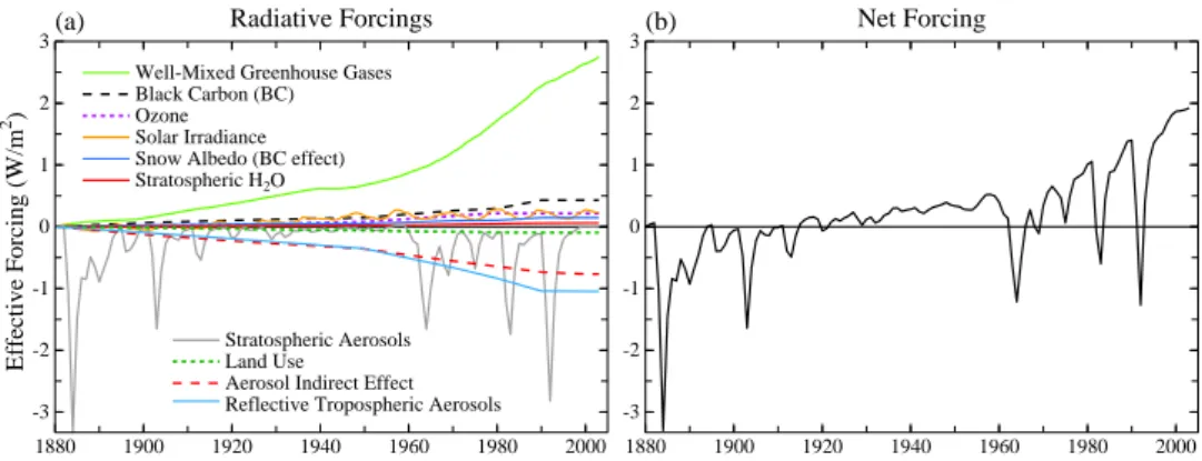
Figure 1 shows the time dependence of the global mean effective forcings. Changes in the quantitative values of these forcings that occur with alternative forcing definitions, which are small in most cases, are discussed in Efficacy (2005) and in conjunction with the transient simulations for 1880–2003 (Hansen et al., 2007a). The predominant forcings are due to GHGs and aerosols, including the aerosol indirect effect. Ozone forcing is significant on the century time scale, and the more uncertain solar forcing may also be important. Volcanic effects are large on short time scales and temporal clustering
1880 1900 1920 1940 1960 1980 2000 -3 -2 -1 0 1 2 3
Well-Mixed Greenhouse Gases Black Carbon (BC) Ozone Solar Irradiance Snow Albedo (BC effect) Stratospheric H2O
Stratospheric Aerosols Land Use Aerosol Indirect Effect Reflective Tropospheric Aerosols
Radiative Forcings Effective Forcing (W/m 2) (a) 1880 1900 1920 1940 1960 1980 2000 -3 -2 -1 0 1 2 3(b) Net Forcing
Fig. 1. Effective global climate forcings (Fe) employed in our global climate simulations, relative to their values in 1880. Use of Fe avoids exaggerating the importance of BC and O3forcings.
of volcanoes contributes to decadal variability. Soot effect on snow and ice albedos and land use change are small global forcings, but can be large on regional scales. Efficacy (2005), this paper, and detailed simulations for 1880–2003 (Hansen et al., 2007a) all use GHG forcings as defined in Fig. 1.
GHG climate forcing, including O3 and CH4-derived stratospheric H2O, is Fe ∼ 3 W/m2. Our partly subjective es-timate of uncertainty, including imprecision in gas amounts and radiative transfer is ∼±15%, i.e. ±0.45 W/m2. Compar-isons with line-by-line radiation calculations (Collins et al., 2006) suggest that the CO2, CH4and N2O forcings in Model III are accurate within several percent, but the CFC forc-ing may be 30–40% too large. If that correction is needed, it will reduce our estimated greenhouse gas forcing to Fe
∼2.9 W/m2.
Stratospheric aerosol forcing following the 1991 Mount Pinatubo volcanic eruption is probably accurate within 20%, based on a strong constraint provided by satellite measure-ments of planetary radiation budget (Wong et al., 2004), as illustrated in Fig. 11 of Efficacy (2005). The uncer-tainty increases for earlier eruptions, reaching about ±50% for Krakatau in 1883. Between large eruptions prior to the satellite era, when small eruptions might escape detec-tion, minimum stratospheric aerosol forcing uncertainty was
∼0.5 W/m2.
Tropospheric aerosols are based on emissions estimates and aerosol transport modeling, as described by Koch (2001). Their indirect effect is a parameterization based on empiri-cal effects of aerosols on cloud droplet number concentra-tion (Menon and Del Genio, 2007) as described in Efficacy (2005). Aerosol forcings are defined in detail by Hansen et al. (2007a). The net direct aerosol forcing is Fe=−0.60 W/m2 and the total aerosol forcing is Fe=−1.37 W/m2 for 1880– 2003. Our largely subjective estimate of the uncertainty in the net aerosol forcing is at least 50%.
The sum of all forcings is Fe∼1.90 W/m2for 1880–2003. However, the net forcing is evaluated more accurately from an ensemble of simulations carried out with all forcings
present at the same time (Efficacy, 2005), thus account-ing for any non-linearity in the combination of forcaccount-ings and minimizing the effect of noise (unforced variability) in the climate model runs. All forcings acting together yield Fe∼1.75 W/m2.
Uncertainty in the net forcing for 1880–2003 is dominated by the aerosol forcing uncertainty, which is at least 50%. Given our estimates, we must conclude that the net forcing is uncertain by ∼1 W/m2. Therefore the smallest and largest forcings within the range of uncertainty differ by more than a factor of three, primarily because of the absence of accurate measurements of aerosol direct and indirect forcings.
One implication of the uncertainty in the net 1880–2003 climate forcing is that it is fruitless to try to obtain an accurate empirical climate sensitivity from observed global tempera-ture change of the past century. However, paleoclimate evi-dence of climate change between periods with well-known boundary conditions (forcings) provides a reasonably pre-cise measure of climate sensitivity: 3±1◦C for doubled CO2 (Hansen et al., 1984, 1993; Hoffert and Covey, 1992). Thus we conclude that our model sensitivity of 2.9◦C for doubled CO2is reasonable.
Figure 1b indicates that, except for occasional large vol-canic eruptions, the GHG climate forcing has become the dominant global climate forcing during the past few decades. GHG dominance is a result of the slowing growth of anthro-pogenic aerosols, as increased aerosol amounts in developing countries have been at least partially balanced by decreases in developed countries. This dominance of GHG forcing, with a net forcing that may be approaching the equivalence of a 1% increase in solar irradiance, implies that global tempera-ture change should now be rising above the level of natural climate variability.
Furthermore, we can anticipate that the dominance of GHG forcing over aerosol and other forcings will be all the more true in the future (Andreae et al., 2005). There is little expectation that developing countries will allow aerosol amounts to continue to grow rapidly, as their aerosol
pollution is already hazardous to human health and tech-nologies to reduce emissions are available. If future GHG amounts are anywhere near the projections in typical IPCC scenarios, GHG climate forcings will be dominant in the fu-ture. Thus, we suggest, it is possible to make meaningful projections of future climate change despite uncertainties in past aerosol forcings.
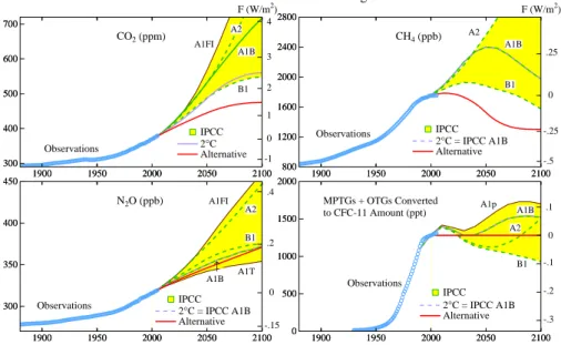
IPCC (2001) defines a broad range of scenarios for future greenhouse gas amounts. This range is shown nominally by the colored area in Fig. 2, which is bordered by the two IPCC scenarios that give the largest and smallest greenhouse gas amounts in 2100. We carry out climate simulations for three IPCC scenarios: A2, A1B and B1. These simulations include changes in well-mixed GHGs only, with short-lived species held fixed at their present values. A2 and B1 are, respec-tively, near the maximum and minimum of the range of IPCC (2001) scenarios, and A1B is known as the IPCC midrange baseline scenario.
We also carry out simulations for the “alternative” and “2◦C” scenarios (Fig. 2) defined in Table 2 of Hansen and Sato (2004). CO2 increases 75 ppm during 2000–2050 in the alternative scenario; CH4decreases moderately, enough to balance a steady increase of N2O; chlorofluorocarbons 11 and 12 decrease enough to balance the increase of all other trace gases, an assumption that is handled by having all these gases remain constant after 2000. CO2 peaks at 475 ppm in 2100 in the alternative scenario, while CH4decreases to 1300 ppb. The alternative scenario is designed to keep the added forcing at about 1 W/m2 in 2000–2050 and another 0.5 W/m2 in 2050–2100. With a nominal climate sensitiv-ity of3/4◦C per W/m2and slowly declining greenhouse gas amounts after 2100, this scenario prevents global warming from exceeding 1◦C above the global temperature in 2000, a level that Hansen (2004, 2005a, b) has argued would con-stitute “dangerous anthropogenic interference” with global climate.
O’Niell and Oppenheimer (2002) suggest 2◦C added global warming as a limit defining “dangerous anthropogenic interference”. Thus we also made climate simulations for a scenario expected to approach but not exceed that limit. The “2◦C” scenario has CO
2peak at 560 ppm in 2100 and other greenhouse gases follow the IPCC midrange scenario A1B (see http://data.giss.nasa.gov/modelforce/ghgases/).
4 Climate simulations
Simulations for the historical period, 1880–2003, warrant careful comparison with observations and analysis of effects of individual forcings. Results are described in detail by Hansen et al. (2007a) and model diagnostics are available at http://data.giss.nasa.gov/modelE/climsim/. We briefly sum-marize results relevant to analysis of the level of future global warming that might constitute dangerous climate interfer-ence.
We emphasize temperature change. Temperature is well measured, it is the variable used in defining climate sensitiv-ity, and our model’s climate sensitivity and capability to sim-ulate observed temperature change are well-tested (Hansen et al., 2007a). Temperature change is important in determin-ing sea level change and movement of the zones in which animal and plant species can survive (Hansen, 2006; Hansen et al., 2006). Changes of the water cycle and climate ex-tremes may be even more important to ecosystems, wildlife and humans, and thus for determination of “dangerous” cli-mate change. We assume that there are systematic changes of the water cycle with global warming. The most impor-tant water cycle changes with global warming are probably intensification of the pattern of precipitation minus evapora-tion and its temporal variance (Held and Soden, 2006; Lu et al. 2007). There is general agreement among a large num-ber of models about the nature of these hydrologic changes with global warming (ibid.), as well as paleoclimate evidence supporting the sense of the changes, and thus we are able to discuss expected water cycle changes with global warming on the basis of temperature projections (Sect. 6.1.2).
The model driven by the forcings of Fig. 1 simulates observed 1880–2003 global temperature change reasonably well, as crudely apparent in Fig. 3a. An equally good fit to observations probably could be obtained from a model with larger sensitivity (than 2.9◦C for doubled CO2)and smaller net forcing, or a model with smaller sensitivity and larger forcing, but paleoclimate evidence constrains climate sensi-tivity, as mentioned above. Also our model responds realis-tically to the known short-term forcing by Pinatubo volcanic aerosols (Hansen et al., 2007a), and simulated global warm-ing for the past few decades, when increaswarm-ing greenhouse gases were the dominant forcing (Fig. 1), is realistic (Hansen et al., 2005b, 2007a).
The largest discrepancies in simulated 1880–2003 surface temperature change are deficient warming in Eurasia and excessive warming of the tropical Pacific Ocean. Hansen et al. (2007a) present evidence that the deficient Eurasian warming may be due to an excessive anthropogenic aerosol optical depth in that region. The lack of notable observed warming in the tropical Pacific could be due to increased fre-quency or intensity of La Ninas (Cane et al., 1997), a char-acteristic that our present model would not be able to capture regardless of whether it was a forced or unforced change.
Overall, simulated climate change does not agree in all de-tails with observations, but such agreement is not expected given unforced climate variability, uncertainty in climate forcings, and current model limitations. However, the cli-mate model does a good job of simulating global tempera-ture change from short time-scale (volcanic aerosol) to cen-tury time-scale forcings. This provides incentive to exam-ine model results for evidence of dangerous human-made cli-mate effects and to investigate how these effects depend upon alternative climate forcing scenarios.
1900 1950 2000 2050 2100 300 400 500 600 700 IPCC 2°C Alternative
Well-Mixed Greenhouse Gas Mixing Ratios
CO2 (ppm) A1FI A2 A1B B1 Observations F (W/m2) 4 3 2 1 0 -1 1900 1950 2000 2050 2100 300 400 500 600 700 1900 1950 2000 2050 2100 800 1200 1600 2000 2400 2800 IPCC 2°C = IPCC A1B Alternative CH4 (ppb) Observations A2 A1B B1 F (W/m2) .25 0 -.25 -.5 1900 1950 2000 2050 2100 800 1200 1600 2000 2400 2800 1900 1950 2000 2050 2100 300 350 400 450 IPCC 2°C = IPCC A1B Alternative N2O (ppb) Observations A1FI A2 B1 A1T A1B↑ .4 .2 0 -.15 1900 1950 2000 2050 2100 300 350 400 450 1900 1950 2000 2050 2100 0 500 1000 1500 2000 IPCC 2°C = IPCC A1B Alternative MPTGs + OTGs Converted
to CFC-11 Amount (ppt) A1p A1B A2 B1 Observations .1 0 -.1 -.2 -.3 1900 1950 2000 2050 2100 0 500 1000 1500 2000
Fig. 2. Observed greenhouse gas amounts as tabulated by Hansen and Sato (2004) and scenarios for the 21st century. Colored area delineates extreme IPCC (2001) scenarios. Alternative and 2◦C scenarios are from Table 2 of Hansen and Sato (2004). MPTGs and OTGs are Montreal Protocol trace gases and other trace gases (Hansen and Sato, 2004). Forcings on right hand scales are adjusted forcings, Fa, relative to values in 2000.
4.1 Global temperature change
We carry out climate simulations for the 21st century and beyond for IPCC (2001) scenarios A2, A1B, and B1 and the “alternative” and “2◦C” scenarios of Hansen et al. (2000) and Hansen and Sato (2004). Simulations are continued beyond 2100 with forcings fixed at 2100 levels as requested by IPCC, although the alternative and 2◦C scenarios per se have a slow decline of human-made forcings after 2100.
Figure 3a and Table 1 show the simulated global mean sur-face air temperature change. The A2 and B1 simulations are single runs, while A1B is a member ensemble. A 5-member ensemble of runs is carried out for the alternative scenario including future volcanoes, the 2010–2100 volcanic aerosols being identical to those of 1910–2000 in the updated Sato et al. (1993) index. Single runs are made for the alter-native and 2◦C scenarios without future volcanoes.
Global warming is 0.80◦C between 2000 and 2100 in the alternative scenario (for the 25-year running mean at 2100; it is 0.66◦C based on linear fit) and 0.89◦C between 2000 and 2200 (0.77◦C based on linear fit) with atmospheric
compo-sition fixed after 2100. The Earth is out of energy balance by ∼3/4W/m2in 2100 (∼0.4 W/m2in 2200) in this scenario (Fig. 3b), so global warming eventually would exceed 1◦C if atmospheric composition remained fixed indefinitely. The alternative scenario of Hansen and Sato (2004) has GHGs decrease slowly after 2100, thus keeping warming <1◦C. Global warming in all other scenarios already exceeds 1◦C by 2100, ranging from 1.2◦C in scenario B1 to 2.7◦C in sce-nario A2.
Note the slow decline of the planetary energy imbalance after 2100 (Fig. 3b), which reflects the shape of the surface temperature response to a climate forcing. Figure 4d in Ef-ficacy (2005) shows that 50% of the equilibrium response is achieved within 25 years, but only 75% after 150 years, and the final 25% requires several centuries. This behavior of the coupled model occurs because the deep ocean contin-ues to take up heat for centuries. Verification of this behav-ior in the real world requires data on deep ocean tempera-ture change. In the model, heat storage associated with this long tail of the response curve occurs mainly in the South-ern Ocean. Measured ocean heat storage in the past decade (Willis et al., 2004; Lyman et al., 2006) presents limited ev-idence of this phenomenon, but the record is too short and the measurements too shallow for full confirmation. Ongo-ing simulations with modelE coupled to the current version of the Bleck (2002) ocean model show less deep mixing of heat anomalies.
Figure 3c compares the global distribution of 21st cen-tury temperature change in the five scenarios. Warming in the alternative scenario is <1◦C in most regions, reaching
1◦C only in the Arctic and a few continental regions. The
weakest IPCC forcing, B1, has almost twice the warming of the alternative scenario, with more than 2◦C in the Arctic. The strongest IPCC forcing, A2, yields four times the global warming of the alternative scenario, with annual warming exceeding 4◦C on large areas of land and in the Arctic. We compare these warmings to observed change and interannual variability in the next section.
1900 1950 2000 2050 2100 2150 2200 14 15 16 17 Individual Runs 5 Run Mean Observations
Surface Air Temperature (°C)
(a)
A2→ A1B B1 IPCC Range w/o Volcanoes ↑ Alternative Scenario with Volcanoes ↑ 2°C Scenario 1900 1950 2000 2050 2100 2150 2200 14 15 16 17 2000 2100 2200 -1 0 1 2 Alternative Scenario 2000 2100 2200 -1 0 1 2 2°C Scenario 2000 2100 2200 -1 0 1 2 IPCC A2 (b) 2000 2100 2200 -1 0 1 2 IPCC A1BNet Radiation at Top of Atmosphre (W/m2)
2000 2100 2200 -1 0 1 2 IPCC B1
Fig. 3. Global mean surface air temperature for several scenarios calculated by our coupled climate model as extensions of the 1880–2003 simulations for “all forcings”. Forcings beyond 2003 for these scenarios are defined in Fig. 2. Stratospheric aerosols in 2010–2100 are the same as in 1910-2000 for the case including future volcanoes. Tropospheric aerosols are unchanging in the 21st century.
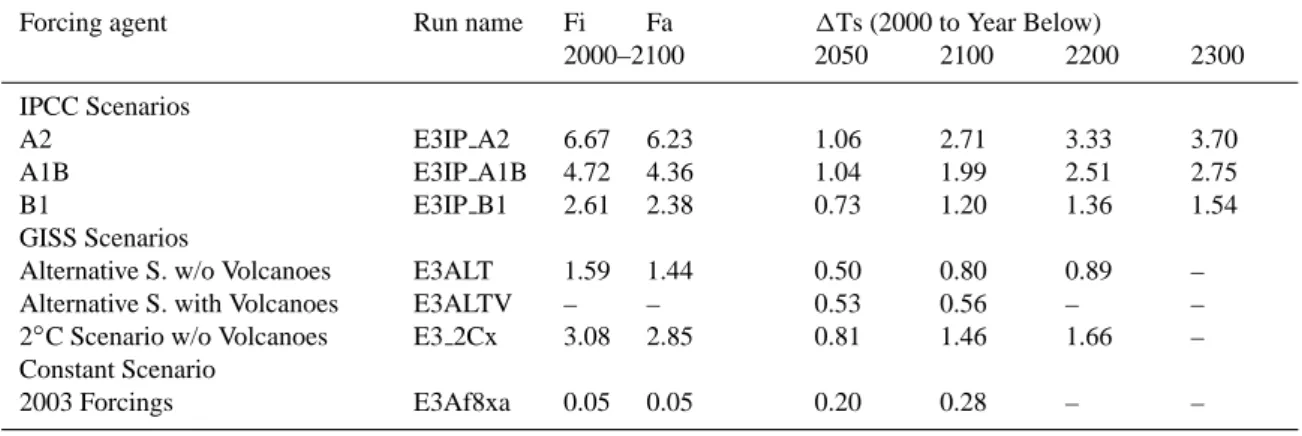
Table 1. Forcings and surface air temperature response to different forcings for several periods in the future.
Forcing agent Run name Fi Fa 1Ts (2000 to Year Below)
2000–2100 2050 2100 2200 2300
IPCC Scenarios
A2 E3IP A2 6.67 6.23 1.06 2.71 3.33 3.70
A1B E3IP A1B 4.72 4.36 1.04 1.99 2.51 2.75
B1 E3IP B1 2.61 2.38 0.73 1.20 1.36 1.54
GISS Scenarios
Alternative S. w/o Volcanoes E3ALT 1.59 1.44 0.50 0.80 0.89 –
Alternative S. with Volcanoes E3ALTV – – 0.53 0.56 – –
2◦C Scenario w/o Volcanoes E3 2Cx 3.08 2.85 0.81 1.46 1.66 –
Constant Scenario
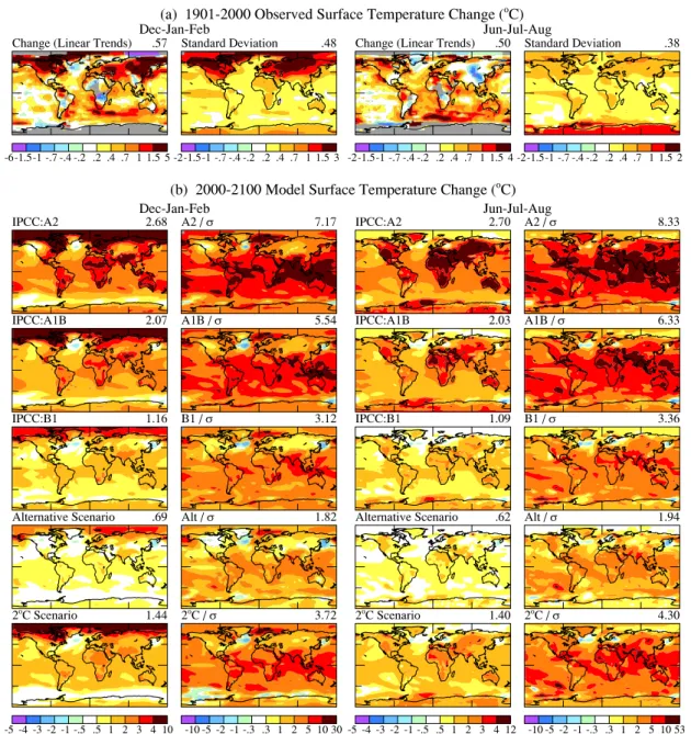
Fig. 4. (a) Observed seasonal (DJF and JJA) surface temperature change in the past century based on local linear trends and the standard deviation about the local 100-year mean temperature, (b) simulated 21st century seasonal temperature change for five GHG scenarios and the ratio of the simulated change to the observed 20th century standard deviation.
4.2 Regional climate change
Figure 4 compares climate change simulated for the present century with climate change and climate variability that hu-mans and the environment experienced in the past century. Figure 4a is the observed change (based on linear trend) of seasonal (winter and summer) surface temperature over the past century and the local standard deviation, σ , of seasonal mean temperature about its 100-year mean. The range within which seasonal-mean temperature has varied in the past mil-lennium is probably no more than twice the range shown in Fig. 4a for the past century (Mann et al., 2003).
Figure 4b shows the simulated change of seasonal mean temperature this century and the ratio of this change to ob-served local temperature variability. Warming in the alterna-tive scenario is typically 2σ or less, i.e. the average seasonal mean temperature at the end of the 21st century will be at a level that is occasionally experienced in today’s climate. Warming in the 2◦C and IPCC B1 scenarios is typically 4σ . Warming in the IPCC A2 and A1B scenarios, commonly called “business-as-usual” (BAU) scenarios, is typically 5– 10σ . Note that due to poorly resolved ENSO variability, σ is underestimated in the tropical Pacific.
Ecosystems, wildlife, and humans would be subjected in the BAU scenarios to conditions far outside their local range of experience. We suggest that 5–10σ changes of seasonal temperature are prima facie evidence that the BAU scenar-ios extend well into the range of “dangerous anthropogenic interference”
Figure 4 provides a general perspective on the magnitude of regional climate change expected for a given climate forc-ing scenario. Additional perspective on the practical signifi-cance of regional climate change is obtained by considering three specific cases: the Arctic, tropical storms originating in the Tropical Atlantic Ocean, and the ocean in the vicinity of ice shelves.
4.2.1 Arctic climate change
Recent warming in the Arctic is having notable effects on regional ecology, wildlife, and indigenous peoples (ACIA, 2004). Unforced climate variability is especially large in the Arctic (Fig. 4, top row), where modeled variability is simi-lar in magnitude to observed variability (Fig. 11 in Hansen et al., 2007a). Observed variability includes the effect of forc-ings, but, at least in the model, forcings are not yet large enough to have noticeable effect on the regional standard de-viation about the long-term trend. Prior to recent warming, the largest fluctuation of Arctic temperature was the brief strong Arctic warming around 1940, which Johannessen et al. (2004) and Delworth and Knutson (2000) argue was an unforced fluctuation associated with the Arctic Oscillation and a resulting positive anomaly of ocean heat inflow into that region. Forcings such as solar variability (Lean and Rind, 1998) or volcanoes (Overpeck et al., 1997) may con-tribute to Arctic variability, but we do not expect details of observed climate change in the first half of the 20th century to be matched by model simulations because of the large un-forced variability. However, the magnitude of simulated Arc-tic warming over the entire century (illustrated by Hansen et al., 2007a) is consistent with observations. Given the attri-bution of at least a large part of global warming to human-made forcings (IPCC, 2001), high latitude amplification of warming in climate models and paleoclimate studies, and the practical impacts of observed climate change (ACIA, 2004), Arctic climate change warrants special attention.
Early energy balance climate models revealed a “small ice cap instability” at the pole (Budyko, 1969; North, 1984), which implied that, once sea ice retreated to a critical lati-tude, all remaining ice would be lost rapidly without addi-tional forcing. This instability disappears in climate mod-els with a seasonal cycle of radiation and realistic dynam-ical energy transports, but a vestige remains: the snow/ice albedo feedback makes sea ice cover in summer and fall sen-sitive to moderate increase of climate forcings. The Arctic was ice-free in the warm season during the Middle Pliocene when global temperature was only 2-3◦C warmer than today (Crowley, 1996; Dowsett et al., 1996).
Satellite data indicate a rapid decline, ∼9%/decade, in perennial Arctic sea ice since 1978 (Comiso, 2002), rais-ing the question of whether the Arctic has reached a “tipprais-ing point” leading inevitably to loss of all warm season sea ice (Lindsay and Zhang, 2005). Indeed, some experts suggest that “. . . there seem to be few, if any, processes or feedbacks that are capable of altering the trajectory toward this ‘super interglacial’ state” free of summer sea ice (Overpeck et al., 2005).
Could the Greenland ice sheet survive if the Arctic were ice-free in summer and fall? It has been argued that not only is ice sheet survival unlikely, but its disintegration would be a wet process that can proceed rapidly (Hansen, 2004, 2005a, b). Thus an ice-free Arctic Ocean, because it may hasten melting of Greenland, may have implications for global sea level, as well as the regional environment, making Arctic cli-mate change centrally relevant to definition of dangerous hu-man interference.
Are there realistic scenarios that might avoid large Arc-tic warming and an ice-free ArcArc-tic Ocean? Efficacy (2005) and Shindell et al. (2006) suggest that non-CO2forcings are the cause of a substantial portion of Arctic climate change, and thus reduction of these pollutants would make stabiliza-tion of Arctic climate more feasible. Investigastabiliza-tion of this topic should include simulations of future climate for plausi-ble changes of forcings that affect the Arctic. Although that is beyond the scope of our present paper, we can make infor-mative comparisons of estimated warmings by greenhouse gases and other pollutants.
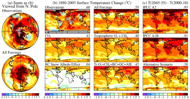
Figure 5a and the top row of Fig. 5b show observed 1880– 2003 surface temperature change and our simulated tempera-ture change for “all forcings”, in both cases the Arctic warm-ing bewarm-ing about twice the global warmwarm-ing. The second row of Fig. 5b shows the results of simulations including only the CO2forcing (left) and only CH4plus tropospheric O3(right). CO2and CH4+O3yield comparable global and Arctic warm-ings. The sum of the responses to CO2and CH4+O3exceeds either observed warming or the simulated warming for “all forcings”, because the real world and “all forcings” include negative forcings, which are due primarily to aerosols.
The lower left of Fig. 5b shows the simulated temper-ature change due to the effect of black carbon on snow albedo. In this simulation, described in detail by Hansen et al. (2007a), a moderate snow albedo forcing (∼0.05 W/m2)is assumed. The BC producing this snow albedo effect also has direct and indirect aerosol forcings, and the sources produc-ing BC also produce OC. The lower right of Fig. 5b shows the simulated temperature change due to the combination of CH4+O3+BC+OC, including aerosol direct and indirect forc-ings and the snow albedo effect. The global warming is about the same as that due to CH4+O3, as the warming by BC and its snow albedo effect is not much larger than the cooling by OC and the indirect effect of BC and OC. Nevertheless, simulated Arctic warming is more than 1◦C with all of these forcings present.
Fig. 5. Surface temperature change based on local linear trends for observations and simulations. (a) is an orthographic projection of the top two maps in (b). CH4forcing includes its indirect effect on stratospheric H2O. Snow albedo effect has 1880–2003 Fa ∼0.05 W/m2. Results in the bottom map of the third column include direct effects of black carbon (BC) and organic carbon (OC) aerosols from fossil fuels and biomass, their aerosol indirect effects (AIE), and the snow albedo effect. (c) shows temperature change in the first half of the 21st century for IPCC BAU and alternative scenarios.
Figure 5c shows that if CO2growth in the 21st century is kept as small as in the alternative scenario, additional Arc-tic warming by 2050 is about the same as warming to date by non-CO2forcings. Thus, in that case, reduction of some of the pollutants considered in Fig. 5 may make it possible to keep further Arctic warming very small and thus probably avoid loss of all sea ice. On the other hand, if CO2growth follows a BAU scenario, the impact of reducing the non-CO2 forcings will be small by comparison and probably inconse-quential.
We suggest that the conclusion that a “tipping point” has been passed, such that it is not possible to avoid a warm-season ice-free Arctic, with all that might entail for regional climate and the Greenland ice sheet, is not warranted yet. Better information is needed on the present magnitude of all anthropogenic forcings and on the potential for their reduc-tion. If CO2 growth is kept close to that of the alternative scenario, and if strong efforts are made to reduce positive non-CO2 forcings, it may be possible to minimize further Arctic climate change.
4.2.2 Tropical climate change
The tropical Atlantic Ocean is the spawning grounds for trop-ical storms and hurricanes that strike the United States and Caribbean nations. Many local and large-scale factors affect storm activity and there are substantial correlations of storm occurrence and severity with external conditions such as the Southern Oscillation and Quasi-Biennial Oscillation (Gray,
1984; Emanuel, 1987; Henderson-Sellers et al., 1998; Gold-enberg, et al., 2001; Trenberth, 2005; Trenberth and Shea, 2006). Two factors especially important for Atlantic hur-ricane activity are SST at 10–20◦N, the main development
region (MDR) for Atlantic tropical storms (Goldenberg, et al., 2001), and the absence of strong vertical wind shear that would inhibit cyclone formation. In addition, SST and ocean temperature to a few hundred meters depth along the hurri-cane track play a role in storm intensity, because warm waters enhance the potential for the moist convection that fuels the storm, while cooler waters at depth stirred up by the storm can dampen its intensity.
Some measures of Atlantic hurricane intensity and dura-tion increased in recent years, raising concern that global warming may be a factor in this trend (Bell et al., 2005; Webster et al., 2005; Emanuel, 2005). However, Gray (2005) and the director of the United States National Hurricane Cen-ter (Mayfield, 2005), while acknowledging a connection be-tween ocean temperature and hurricanes, reject the sugges-tion that global warming has contributed to the recent storm upsurge, citing instead natural cycles of Atlantic Ocean tem-perature. Indeed, multi-decadal variations of Atlantic Ocean temperatures are found in instrumental data (Kushnir, 1994), in paleoclimate proxy temperatures (Mann et al., 1998), and in coupled atmosphere-ocean climate simulations with-out external forcing (Delworth and Mann, 2000). How-ever, Mann and Emanuel (2006) argue that the attribution of observed SST fluctuations in the MDR associated with the Atlantic Multi-decadal Oscillation is a statistical
arti-fact, and that practically all SST variability in the region can be attributed to competing trends in greenhouse gases and aerosols.
Climate forcings also contribute to ocean temperature change, so it is of interest to compare modeled temperature change due to forcings with observed temperature change in regions and seasons relevant to tropical storms. Bell et al. (2005) define an Accumulated Cyclone Energy (ACE) index that accounts for the combined strength and duration of tropical storms of hurricanes originating in the Atlantic Ocean. This index (Fig. 4.5 of Bell et al., 2005) was gen-erally low during 1970–1994. For the past decade the ACE index has been a factor 2.4 higher than in 1970–1994. Per-haps not coincidentally, the index had peaks near 1980 and 1990, when global temperature also had peaks, and the index was low during the few years affected by the 1991 Pinatubo global cooling. The past decade, when ACE is highest, is the warmest time in the past century and a period with rapid up-take of heat by the ocean (Levitus et al., 2005; Willis et al., 2004; Hansen et al., 2005b; Lyman et al., 2006).
Figure 6a shows SST anomalies in 1995–2005, the time of high hurricane intensity, relative to 1970–1994, when At-lantic Ocean and Gulf of Mexico hurricanes were weaker. Observations have warming ∼0.2◦C in the Gulf of Mexico and ∼0.45◦C in the MDR. The ensemble mean of the simu-lation with standard “all forcings” has warming about 0.35◦C in both regions, suggesting that much, perhaps most, of ob-served warming in these critical regions is due to the forcings that drive the climate model. Increasing GHGs, the princi-pal forcing driving the model toward warming (Fig. 1), are known accurately, but other forcings have large uncertainties. Thus we performed additional simulations in which the most uncertain forcings were altered to test the effect of uncer-tainties and to provide more fodder for examining statistical significance.
The lower three rows in Figs. 6a (and 6c) show results for three 5-member ensembles of model runs with altered tro-pospheric aerosol and solar forcings, as described in detail by Hansen et al. (2007a). In AltAer1 anthropogenic sulfate aerosols have the identical time dependence as in the stan-dard experiment (Fig. 1) but the anthropogenic increase is reduced by 50%. AltAer2 adds to AltAer1 a doubling of the temporal increase of biomass burning aerosols. AltSol replaces the solar irradiance history of Lean (2000), which includes both long-term and solar cycle variations, with the time series of Lean et al. (2002), which retains only the solar change due to the 11-year Schwabe cycle. These alternative forcings all yield ensemble-mean SST warmings in the MDR comparable to that with standard forcings.
Figure 6b shows the 1995–2005 temperature anomalies in the five individual runs with “all forcings”, each of which yields warming in both the Gulf of Mexico and the MDR. Figure 6c shows the standard deviations σ * among succes-sive 10-year periods relative to the preceding 25 years within the available relevant period of record (1900–1994). As
ex-pected, the model has too little variability at low latitudes, but it is more realistic at middle and high latitudes (the small “observed” SST variability at the highest latitudes is an artifi-cial result of specifying a fixed SST if any sea ice is present).
σ* is ∼0.15◦C in the Gulf of Mexico in observations and model. Observed σ * is ∼0.25◦C in the MDR, but only about half that large in the model.
In summary, the warming in the model in recent decades is due to the assumed forcings, and Hansen et al. (2007a) present evidence that the magnitude of the model’s response to forcings is realistic on time scales from that for individual volcanic eruptions to multidecadal GHG increases. The pe-riod 1970–2005 under discussion with regard to hurricanes is the time when forcings are known most accurately, and dur-ing that period anthropogenic GHGs were the dominant forc-ing. Although unforced fluctuations undoubtedly contribute to Atlantic Ocean temperature change, the expected GHG warming is comparable in magnitude to observed warming and must be at least a significant contributor to that warm-ing.
We conclude that the definitive assertion of Gray (2005) and Mayfield (2005), that human-made GHGs play no role in the Atlantic Ocean temperature changes that they assume to drive hurricane intensification, is untenable. Specifically, the assertions that (1) hurricane intensification of the past decade is due to changes in SST in the Atlantic Ocean, and (2) global warming cannot have had a significant role in the hurricane intensification of the past decade, are mutually in-consistent. On the contrary, although natural cycles play a role in changing Atlantic SST, our model results indicate that, to the degree that hurricane intensification of the past decade is a product of increasing SST in the Atlantic Ocean and the Gulf of Mexico, human-made GHGs probably are a substantial contributor, as also concluded by Mann and Emanuel (2006). Santer et al. (2006) have obtained similar conclusions by examining the results of 22 climate models.
Figure 6d shows the additional SST warming during hur-ricane season by mid-century in the three IPCC, alterna-tive, and 2◦C scenarios, relative to the present. SST is only one of the environmental factors that affect hurricanes, but there is theoretical (Emanuel, 1987) and empirical evidence (Emanuel, 2005; Webster et al., 2005) that higher SST con-tributes to increased maximum strength of tropical cyclones. The salient point that we note in Fig. 6d is that, despite the fact that warming “in the pipeline” in 2004 is the same for all scenarios, the alternative scenario already at mid-century has notably less warming than the other scenarios. This result refutes the common statement that constraining climate forc-ings has a negligible effect on expected warming this century. Divergence of warming among the scenarios is even greater in later decades, as the growth of climate forcing declines rapidly in the alternative scenario, thus making that scenario less “dangerous” to the extent that SST influences storm in-tensity.
Fig. 6. (a) 1995–2005 August–October SST anomalies relative to 1970–1994 base period, the top map for observations and next four for several “all forcing” ensembles, (b) 1995–2005 August–October SST anomalies relative to 1970–1994 for individual ensemble members of the standard “all forcings” simulation, (c)standard deviations among successive decadal means relative to immediately preceding 25 years, (d) simulated 2045–2055 August–October SST anomalies relative to the present (2001–2009 mean).
4.2.3 Ice sheet and methane hydrate stabilities
Perhaps the greatest threat of catastrophic climate impacts for humans is the possibility that warming may cause one or more of the ice sheets to become unstable, initiating a process of disintegration that is out of humanity’s control. We focus on ice sheet stability, because of the potential for sea level to change this century. However, ice sheet stability is related to the stability of methane hydrates in permafrost and in marine sediments, because ice sheet disintegration and methane re-lease are both affected by surface warming at high latitudes and by ocean warming at depths that affect ice shelves and shallow methane hydrate deposits. Also, a substantial pos-itive climate feedback from methane release could make it difficult to achieve the relatively benign alternative scenario, thus affecting the ice sheet stability issue as well as other cli-mate impacts. Most methane hydrates in marine sediments are at depths beneath the ocean floor that would require
cen-turies for destabilization (Kvenvolden and Lorenson, 2001; Archer, 2007), but the anthropogenic thermal burst in ocean temperatures is likely to persist for centuries. Furthermore, the methane in shallow sediments, i.e. at or near the sea floor, might begin to yield a positive climate feedback this century if substantial warm thermal anomalies penetrate to the ocean bottom.
The Greenland and Antarctic ice sheets contain enough water to raise sea level about 70 m, with Greenland and West Antarctica each containing about 10% of the total and East Antarctica holding the remaining 80%. IPCC (2001) central estimates for sea level change in the 21st century include neg-ligible contributions from Greenland and Antarctica, as they presume that melting of ice sheet fringes will be largely bal-anced by ice sheet growth in interior regions where snowfall increases.
However, Earth’s history shows that the long-term re-sponse to global warming includes substantial melting of
ice and sea level rise. During the penultimate interglacial period, ∼130 000 years ago, when global temperature may have been as much as ∼1◦C warmer than in the present
inter-glacial period, sea level was 4±2 m higher than today (Mc-Culloch and Esat, 2000; Thompson and Goldstein, 2005), demonstrating that today’s sea level is not particularly fa-vored. However, changes of sea level and global temperature among recent interglacial periods are not large compared to the uncertainties, and ice sheet stability is affected not only by global temperature but also by the geographical and sea-son distribution of solar irradiance, which differ from one in-terglacial period to another. Therefore, it is difficult to use the last interglacial period as a measure of the sensitivity of sea level to global temperature. The most recent time with global temperature ∼3◦C greater than today (during the Pliocene,
∼3 million years ago) had sea level 25±10 m higher than to-day (Barrett et al., 1992; Dowsett et al. 1994; Dwyer et al., 1995), suggesting that, given enough time, a BAU level of global warming could yield huge sea level change. A prin-cipal issue is thus the response time of ice sheets to global warming.
It is commonly assumed, perhaps because of the time scale of the ice ages, that the response time of ice sheets is millen-nia. Indeed, ice sheet models designed to interpret slow pa-leoclimate changes respond lethargically, i.e. on millennial time scales. However, perceived paleoclimate change may reflect more the time scale for changes of forcing, rather than an inherent ice sheet response time. Ice sheet models used for paleoclimate studies generally do not incorporate all the physics that may be critical for the wet process of ice sheet disintegration, e.g. modeling of the ice streams that chan-nel flow of continental ice to the ocean, including effects of melt percolation through crevasses and moulins, removal of ice shelves by the warming ocean, and dynamical propaga-tion inland of the thinning and retreat of coastal ice. Hansen (2005a,b) argues that, for a forcing as large as that in BAU climate forcing scenarios, a large ice sheet response would likely occur within centuries, and ice melt this century could yield sea level rise of 1 m or more and a dynamically chang-ing ice sheet that is out of our control.
Two regional climate changes particularly relevant to ice sheet response time are: (1) surface melt on the ice sheets, and (2) melt of submarine ice shelves that buttress glaciers draining the ice sheets. Zwally et al. (2002) showed that increased surface melt on Greenland penetrated ice sheet crevasses and reached the ice sheet base, where it lubri-cated the ice-bedrock interface and accelerated ice discharge to the ocean. Van den Broeke (2005) found that unusu-ally large surface melt on an Antarctic ice shelf preceded and probably contributed significantly to collapse of the ice shelf. Thinning and retreat of ice shelves due to warming ocean water works in concert with surface melt. Hughes (1972, 1981) and Mercer (1978) suggested that floating and grounded ice shelves extending into the ocean serve to but-tress outlet glaciers, and thus a warming ocean that melts
ice shelves could lead to rapid ice sheet shrinkage or col-lapse. Confirmation of the effectiveness of these processes has been obtained in the past decade from observations of increased surface melt, ice shelf thinning and retreat, and ac-celeration of glaciers on the Antarctic Peninsula (De Ange-lis and Skvarca, 2003; Rignot et al., 2004; van den Broeke, 2005), West Antarctica (Rignot, 1998; Shepherd et al., 2002, 2004; Thomas et al., 2004), and Greenland (Abdalati et al., 2001; Zwally et al., 2002; Thomas et al., 2003), in some cases with documented effects extending far inland. Thus we examine here both projected surface warming on the ice sheets and warming of nearby ocean waters.
Summer surface air temperature change on Greenland in the 21st century is only 0.5–1◦C with alternative scenario cli-mate forcings (Fig. 4), but it is 2–4◦C for the IPCC BAU sce-narios (A2 and A1B). Simulated 21st century summer warm-ings in West Antarctica (Fig. 4) differ by a similar factor, be-ing ∼0.5◦C in the alternative scenario and ∼2◦C in the BAU
scenarios.
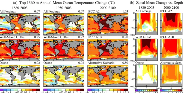
Submarine ice shelves around Antarctica and Greenland extend to ocean depths of 1 km and deeper (Rignot and Ja-cobs, 2002). Figure 7b shows simulated zonal mean ocean temperature change versus depth for the past century and the 21st century. Despite near absence of surface warming in the Antarctic Circumpolar Current, warming of a few tenths of a degree is found at depths from a few hundred to 1500 m, consistent with observations in the past half-century (Gille, 2002; Aoki et al., 2003). Modeled warming is due to GHGs, with less warming when all forcings are included.
Maps of simulated temperature change for the top 1360 m of the ocean (Fig. 7a) show warming around the entire cir-cumference of Greenland, despite cooling in the North At-lantic. This warming at ocean depth differs by about a fac-tor of two between the alternative and BAU scenarios, less than the factor ∼4 difference in summer surface warming over Greenland and Antarctica, consistent with the longer re-sponse time of the ocean. Although we cannot easily convert temperature increase into rate of melting and sea level rise, it is apparent that the BAU scenarios pose much greater risk of large sea level rise than the alternative scenario, as discussed in Sect. 6.
Surface and submarine temperature change are also rele-vant to the stability of methane hydrates in permafrost and in ocean sediments. Recent warming is already beginning to cause release of methane from thawing permafrost in Siberia (Walter et al., 2006; Zimov et al., 2006), with similar en-hancements due to permafrost and vegetation changes in Scandinavia (Christensen et al., 2004), but this methane re-lease is not yet large enough to yield an overall increase of atmospheric CH4, as shown in Sect. 5. Projected 21st century summer warming in the Northern Hemisphere permafrost re-gions is typically a factor of five larger in BAU scenarios than in the alternative scenario (Fig. 4), suggesting that the threat of a significant positive climate feedback is much greater in the BAU scenarios.
Fig. 7. (a) Temperature change in the top 10 layers (1360 m) of the ocean for three periods and three forcings, (b) zonal-mean ocean temperature change for these forcings. Positive and negative temperature intervals are symmetric about zero.
Methane hydrates in ocean sediments are an even larger potential source of methane emissions (Archer, 2007). It is possible that much of the temperature rise in extreme global warming events, such as the approximately 6◦C that occurred at the Paleocene-Eocene boundary about 55 million years ago (Bowen et al., 2006), resulted from catastrophic release of methane from methane hydrates in ocean sediments. It may require many centuries for ocean warming to substan-tially impact these methane hydrates (Archer, 2007). Cal-culations of global warming enhancement from methane hy-drates based on diffusive or upwelling-diffusion ocean mod-els suggest that the methane hydrate feedback is small on the century time scale (Harvey and Huang, 1995). How-ever, the positive thermal anomalies that we simulate with our dynamic ocean model at great ocean depths at high lati-tudes (Fig. 7) are much larger near the ocean bottom than we would obtain with diffusive mixing of anomalies (as in our Q-flux model), suggesting that further attention to the pos-sibility of methane hydrate release is warranted. With our present lack of understanding, we can perhaps only say with reasonable confidence that the chance of significant methane hydrate feedback is greater with BAU scenarios than with the alternative scenario, and that empirical evidence from prior interglacial periods suggests that large methane hydrate re-lease is unlikely if global warming is kept within the range of recent interglacial periods.
5 Actual GHG trends versus scenarios
Global and regional climate changes simulated for IPCC sce-narios in the 21st century are large in comparison with
ob-served climate variations in the 20th century. This raises the question: is it plausible for global climate forcing to follow a path with a smaller forcing than those in the IPCC scenarios? 5.1 Ambient GHG amounts
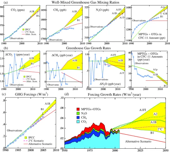
Figure 8a compares GHG scenarios and observations, the lat-ter being an update of Hansen and Sato (2004) (see http: //data.giss.nasa.gov/modelforce/ghgases/), who define the data sources and methods of obtaining global means from station measurements. Figure 8b shows the corresponding annual growth rates. Figures 8c and d compare observed cli-mate forcings and their growth rates with the IPCC, 2◦C, and alternative scenarios.
Observed CO2 falls close to all scenarios, which do not differ much in early years of the 21st century. CO2has large year-to-year variations in its growth rate due to variations in terrestrial and ocean sinks, as well as biomass burning and fossil fuel sources. However, we are able to draw conclu-sions in Sect. 5.3 about the realism of CO2scenarios by com-paring emission scenarios with real world data on fossil fuel CO2emission trends, for which there are reasonably accurate data.
Overall, growth rates of the well-mixed non-CO2forcings fall below IPCC scenarios (Figs. 8a, b). Growth of CH4 falls below any IPCC scenario and even below the alterna-tive scenario. Observed N2O falls slightly below all scenar-ios. The sum of MPTGs (Montreal Protocol Trace Gases) and OTGs (Other Trace Gases) falls between the IPCC sce-narios and the alternative scenario (which was defined at a later time than the IPCC scenarios, when more observational data were available). The estimated forcing by MPTGs is
1990 2000 2010 360 370 380 390 IPCC IPCC 2°C Scen. Alter. Scen. CO2 (ppm) A1B ↑ B1 Observations (a) 1990 2000 2010 360 370 380 390 1990 2000 2010 1700 1750 1800 1850 CH4 (ppb) Observations A1B B1
Well-Mixed Greenhouse Gas Mixing Ratios
1990 2000 2010 1700 1750 1800 1850 1990 2000 2010 310 315 320 325 N2O (ppb) Observations A1FI A1T ↑ A1B → 1990 2000 2010 310 315 320 325 1990 2000 2010 1100 1200 1300 1400 MPTGs + OTGs in CFC-11 Amount (ppt) A1p ↑ A1B ↑ B1 Observations 1990 2000 2010 1100 1200 1300 1400 1990 2000 2010 1.0 1.5 2.0 2.5 3.0 IPCC 2°C Scen. Alter. Scen. ∆CO2 (ppm/year) A1B B1 Observations (b) 1990 2000 2010 1.0 1.5 2.0 2.5 3.0 1990 2000 2010 0 5 10 15 ∆CH 4 (ppb/year) Observatns A1B B1
Greenhouse Gas Growth Rates
1990 2000 2010 0 5 10 15 1990 2000 2010 .0 .5 1.0 ∆N2O (ppb/year) Observations A1FI A1T A1B 1990 2000 2010 .0 .5 1.0 1990 2000 2010 -10 0 10 20 30 40 MPTGs + OTGs in CFC-11 Amounts (ppt/year) A1p A1B B1 Observations 1990 2000 2010 -10 0 10 20 30 40 1990 1995 2000 2005 2010 .0 .2 .4 .6 .8 IPCC 2°C Scenario Alternative Scenario GHG Forcings (W/m2) (c) A1B B1 Observations ↓ 1990 1995 2000 2005 2010 .0 .2 .4 .6 .8 1950 1975 2000 2025 2050 .00 .02 .04 .06 .08 .10 MPTGs+OTGs N2O CH4 CO2
Forcing Growth Rates (W/m2/year) (d) A1B A1FI B1 2°C Alternative Scenario A2 1950 1975 2000 2025 2050 .00 .02 .04 .06 .08 .10
Fig. 8. (a) Greenhouse gas amounts, (b) growth rates, and (c) resulting forcings and (d) forcing growth rates for IPCC (2001), “alternative”, and “2◦C” scenarios (Hansen et al., 2000; Hansen and Sato, 2004). Observations in (d) are 5-year running means of data described by Hansen and Sato (2004) and in the text. Data for recent decades are those reported by the NOAA Earth System Research Laboratory, Global Monitoring Division (http://www.cmdl.noaa.gov/). MPTGs and OTGs without available observations (4.9% of the MPTG + OTG estimated forcing in 2000) were assumed to follow IPCC scenario A1B, which probably exaggerates their forcing, as all measured MPTGs and OTGs are currently falling below their IPCC scenarios.
based on measurements of 10 of these gases, as delineated by Hansen and Sato (2004), all of which are growing more slowly than in the IPCC scenarios, with the few significant unmeasured MPTGs assumed to follow the lowest IPCC sce-nario. OTGs with reported data include HFC-134a and SF6, for which measurements are close to or slightly below IPCC scenarios.
Figures 8c and d show that the net forcing by well-mixed GHGs for the past few years has been following a course close to that of the alternative scenario. However, it should not be assumed that forcings will remain close to the alter-native scenario, because, as shown below, fossil fuel CO2 emissions now substantially exceed those in the alternative scenario.
The alternative scenario was defined (Hansen et al., 2000) as a potential goal under the assumption of concerted global efforts to simultaneously (1) reduce air pollution (for hu-man health, climate and other reasons), and (2) stabilize CO2
emissions initially and begin to achieve significant emission reductions before mid-century, such that added CO2forcing is held to ∼1 W/m2in 50 years and ∼1.5 W/m2in 100 years. Thus the alternative scenario assumes that CH4amount will peak within a decade and then decline enough to balance continued growth of N2O. It also assumes that the decline of CH4 and other O3precursors will decrease tropospheric O3enough to balance the small increase in forcing (several hundredths of a W/m2)expected due to recovery of halogen-induced stratospheric O3depletion.
The most demanding requirement of the alternative sce-nario is that added CO2forcing be held to ∼1 W/m2 in 50 years and ∼1.5 W/m2 in 100 years. The scenario in our present climate simulations, for example, has annual mean CO2growth of 1.7 ppm/year at the end of the 20th century declining to 1.3 ppm/year by 2050. The plausibility of the alternative scenario thus depends critically upon fossil fuel CO2emissions.
0 20 40 60 80 100 0 20 40 60 80
100 (a) Decay of Pulse CO2 Emission
Year
Remaining Fraction (%)
Carbon Cycle Constraints
Fit to Bern Carbon Cycle Model
CO2(t) = 18 + 14 exp(-t/420) + 18 exp(-t/70) + 24 exp(-t/21) + 26 exp(-t/3.4) 33% ↓ Remaining Airborne 22% at 500 years 19% at 1000 years 0 200 400 600 800 1000 1200 1400 Reserve Growth Proven Reserves Emissions (1750-2005)
(b) Fossil Fuel Reservoirs
Gt C
Oil Gas Coal Other
IPCC EIA ? Methane Hydrates Shale Oil Tar Sands 0 100 200 300 400 500 600 CO 2 (ppm)
Fig. 9. (a) Decay of a small pulse of CO2added to today’s atmosphere, based on analytic approximation to the Bern carbon cycle model (Joos et al., 1996; Shine et al., 2005), (b) fossil fuel emissions to date based on sources in Fig. 9, and proven reserves and estimated economically recoverable reserve growth based on EIA (2005) and, in the case of coal, IPCC (2001).
5.2 Fossil fuel CO2emissions
Global fossil fuel CO2emissions change by only a few per-cent per year and are known with sufficient accuracy that we can draw conclusions related to atmospheric CO2trends, despite large year-to-year variability in atmospheric CO2 growth. In recent decades the increase of atmospheric CO2, averaged over several years, has been ∼58% of fossil fuel emissions (IPCC, 2001; Hansen, 2005b). Carbon cycle mod-els suggest that this “airborne fraction” of CO2 is unlikely to decrease this century if emissions increase, indeed, most models yield an increasing airborne fraction as terrestrial CO2uptake is likely to decrease (Cox et al., 2000; Friedling-stein, et al., 2003; Fung et al., 2005; Matthews et al., 2005; Jones et al., 2005).
Carbon cycle facts sketched in Fig. 9 aid discussion of the role of fossil fuel CO2emissions in determining future cli-mate forcing, and specifically help define constraints on CO2 emissions that are needed if the alternative scenario is to be achieved. Figure 9a shows the decay of a small pulse CO2 emission based on a simple analytic fit to the Bern carbon cycle model (Joos et al., 1996)
CO2(%)=18+14e−t /420+18e−t /70+24e−t /21+26e−t /3.4. (1) In Eq. (1), t is time, and we slightly rounded coefficients calculated by Joos (Shine et al., 2005).
In this approximation of the carbon cycle, about one-third of anthropogenic CO2 emissions remain in the atmosphere after 100 years (Fig. 9a) and one-fifth after 1000 years. Pro-cesses not accounted for by the model, including burial of carbon in ocean sediments from perturbation of the CaCO3 cycle and silicate weathering, remove CO2 on longer time scales (Archer, 2005), but for practical purposes 500–1000 years is “forever”, as it is long enough for ice sheets to re-spond and it is many human generations. Indeed, Eq. (1) should be viewed as an approximate lower bound for the portion of fossil fuel CO2 emissions that remain airborne.
The uptake capacity of the ocean decreases as the amount of dissolved carbon increases (the buffer factor increases) and there are uncertain but potentially large climate feedbacks that may add CO2to the air, e.g. carbon emissions from for-est dieback (Cox et al., 2000), melting permafrost (Walter et al., 2006; Zimov et al., 2006), and warming ocean bottom (Archer, 2007).
Integration over the period 1750–2005 of the product of Eq. (1) and fossil fuel emissions yields a present airborne fossil fuel CO2amount of ∼80 ppm. (Kharecha and Hansen, 2007) The observed atmospheric CO2increase is ∼100 ppm, the difference presumably due to the net consequence of de-forestation and biospheric uptake not incorporated in the car-bon cycle model, and, in part, imprecision of the carcar-bon cycle model. This calculation provides a check on the reasonable-ness of the carbon cycle model approximation of Eq. (1), which should continue to provide useful estimates for the moderate fossil fuel emissions inherent in the alternative sce-nario. As mentioned above, for the greater CO2emissions of BAU scenarios Eq. (1) may begin to substantially underes-timate airborne CO2, as it excludes the nonlinearity of the ocean carbon cycle and anticipated climate feedbacks on at-mospheric CO2and CH4, the latter being eventually oxidized to CO2.
Figure 9b suggests the key role that coal and unconven-tional fossil fuels (labeled “other”) will play in determining future CO2 levels and the attainment or non-attainment of the alternative scenario. If growth of oil and gas reserves estimated by the Energy Information Administration (EIA, 2005) is realistic, full exploitation of oil and gas will take air-borne atmospheric CO2to ∼450 ppm, assuming that coal use is phased out over the next several decades except for uses where the CO2 produced can be captured and sequestered. (Kharecha and Hansen, 2007) Achievement of this CO2limit also requires that the massive amounts of unconventional fos-sil fuels (labeled “other” in Fig. 9) are exploited only if the resulting CO2is captured and sequestered.