Lecture Notes
Erich Miersemann Department of Mathematics
Leipzig University Version October, 2012
Contents
1 Introduction 9 1.1 Problems in Rn . . . . 9 1.1.1 Calculus . . . 9 1.1.2 Nash equilibrium . . . 10 1.1.3 Eigenvalues . . . 101.2 Ordinary differential equations . . . 11
1.2.1 Rotationally symmetric minimal surface . . . 12
1.2.2 Brachistochrone . . . 13
1.2.3 Geodesic curves . . . 14
1.2.4 Critical load . . . 15
1.2.5 Euler’s polygonal method . . . 20
1.2.6 Optimal control . . . 21
1.3 Partial differential equations . . . 22
1.3.1 Dirichlet integral . . . 22
1.3.2 Minimal surface equation . . . 23
1.3.3 Capillary equation . . . 26
1.3.4 Liquid layers . . . 29
1.3.5 Extremal property of an eigenvalue . . . 30
1.3.6 Isoperimetric problems . . . 31
1.4 Exercises . . . 33
2 Functions of n variables 39 2.1 Optima, tangent cones . . . 39
2.1.1 Exercises . . . 45 2.2 Necessary conditions . . . 47 2.2.1 Equality constraints . . . 49 2.2.2 Inequality constraints . . . 52 2.2.3 Supplement . . . 56 2.2.4 Exercises . . . 58 3
2.3 Sufficient conditions . . . 59 2.3.1 Equality constraints . . . 61 2.3.2 Inequality constraints . . . 62 2.3.3 Exercises . . . 64 2.4 Kuhn-Tucker theory . . . 65 2.4.1 Exercises . . . 71 2.5 Examples . . . 72 2.5.1 Maximizing of utility . . . 72 2.5.2 V is a polyhedron . . . 73 2.5.3 Eigenvalue equations . . . 73
2.5.4 Unilateral eigenvalue problems . . . 77
2.5.5 Noncooperative games . . . 79
2.5.6 Exercises . . . 83
2.6 Appendix: Convex sets . . . 90
2.6.1 Separation of convex sets . . . 90
2.6.2 Linear inequalities . . . 94
2.6.3 Projection on convex sets . . . 96
2.6.4 Lagrange multiplier rules . . . 98
2.6.5 Exercises . . . 101
2.7 References . . . 103
3 Ordinary differential equations 105 3.1 Optima, tangent cones, derivatives . . . 105
3.1.1 Exercises . . . 108
3.2 Necessary conditions . . . 109
3.2.1 Free problems . . . 109
3.2.2 Systems of equations . . . 120
3.2.3 Free boundary conditions . . . 123
3.2.4 Transversality conditions . . . 125
3.2.5 Nonsmooth solutions . . . 129
3.2.6 Equality constraints; functionals . . . 134
3.2.7 Equality constraints; functions . . . 137
3.2.8 Unilateral constraints . . . 141
3.2.9 Exercises . . . 145
3.3 Sufficient conditions; weak minimizers . . . 149
3.3.1 Free problems . . . 149
3.3.2 Equality constraints . . . 152
3.3.3 Unilateral constraints . . . 155
3.3.4 Exercises . . . 162
3.4.1 Exercises . . . 169
3.5 Optimal control . . . 170
3.5.1 Pontryagin’s maximum principle . . . 171
3.5.2 Examples . . . 171
3.5.3 Proof of Pontryagin’s maximum principle; free endpoint176 3.5.4 Proof of Pontryagin’s maximum principle; fixed end-point . . . 179
Preface
These lecture notes are intented as a straightforward introduction to the calculus of variations which can serve as a textbook for undergraduate and beginning graduate students.
The main body of Chapter 2 consists of well known results concerning necessary or sufficient criteria for local minimizers, including Lagrange mul-tiplier rules, of real functions defined on a Euclidean n-space. Chapter 3 concerns problems governed by ordinary differential equations.
The content of these notes is not encyclopedic at all. For additional reading we recommend following books: Luenberger [36], Rockafellar [50] and Rockafellar and Wets [49] for Chapter 2 and Bolza [6], Courant and Hilbert [9], Giaquinta and Hildebrandt [19], Jost and Li-Jost [26], Sagan [52], Troutman [59] and Zeidler [60] for Chapter 3. Concerning variational prob-lems governed by partial differential equations see Jost and Li-Jost [26] and Struwe [57], for example.
Introduction
A huge amount of problems in the calculus of variations have their origin in physics where one has to minimize the energy associated to the problem under consideration. Nowadays many problems come from economics. Here is the main point that the resources are restricted. There is no economy without restricted resources.
Some basic problems in the calculus of variations are:
(i) find minimizers,
(ii) necessary conditions which have to satisfy minimizers,
(iii) find solutions (extremals) which satisfy the necessary condition, (iv) sufficient conditions which guarantee that such solutions are minimizers, (v) qualitative properties of minimizers, like regularity properties,
(vi) how depend minimizers on parameters?,
(vii) stability of extremals depending on parameters.
In the following we consider some examples.
1.1
Problems in R
n1.1.1 Calculus
Let f : V 7→ R, where V ⊂ Rn is a nonempty set. Consider the problem x∈ V : f(x) ≤ f(y) for all y ∈ V.
If there exists a solution then it follows further characterizations of the solution which allow in many cases to calculate this solution. The main tool
for obtaining further properties is to insert for y admissible variations of x. As an example let V be a convex set. Then for given y∈ V
f (x)≤ f(x + ²(y − x))
for all real 0≤ ² ≤ 1. From this inequality one derives the inequality h∇f(x), y − xi ≥ 0 for all y ∈ V,
provided that f ∈ C1(Rn).
1.1.2 Nash equilibrium
In generalization to the above problem we consider two real functions fi(x, y),
i = 1, 2, defined on S1× S2, where Si⊂ Rmi. An (x∗, y∗)∈ S1× S2 is called
a Nash equilibrium if
f1(x, y∗) ≤ f1(x∗, y∗) for all x∈ S1
f2(x∗, y) ≤ f2(x∗, y∗) for all y∈ S2.
The functions f1, f2 are called payoff functions of two players and the sets
S1and S2 are the strategy sets of the players. Under additional assumptions
on fi and Si there exists a Nash equilibrium, see Nash [46]. In Section 2.4.5
we consider more general problems of noncooperative games which play an important role in economics, for example.
1.1.3 Eigenvalues
Consider the eigenvalue problem
Ax = λBx,
where A and B are real and symmetric matrices with n rows (and n columns). Suppose thathBy, yi > 0 for all y ∈ Rn\ {0}, then the lowest eigenvalue λ
1 is given by λ1= min y∈Rn\{0} hAy, yi hBy, yi.
The higher eigenvalues can be characterized by the maximum-minimum principle of Courant, see Section 2.5.
In generalization, let C⊂ Rnbe a nonempty closed convex cone with vertex
at the origin. Assume C 6= {0}. Then, see [37], λ1 = min
y∈C\{0}
hAy, yi hBy, yi
is the lowest eigenvalue of the variational inequality
x∈ C : hAx, y − xi ≥ λhBx, y − xi for all y ∈ C.
Remark. A set C ⊂ Rn is said to be a cone with vertex at x if for any
y∈ C it follows that x + t(y − x) ∈ C for all t > 0.
1.2
Ordinary differential equations
Set
E(v) = Z b
a
f (x, v(x), v0(x)) dx
and for given ua, ub ∈ R
V ={v ∈ C1[a, b] : v(a) = ua, v(b) = ub},
where −∞ < a < b < ∞ and f is sufficiently regular. One of the basic problems in the calculus of variation is
(P ) minv∈V E(v).
That is, we seek a
u∈ V : E(u) ≤ E(v) for all v ∈ V.
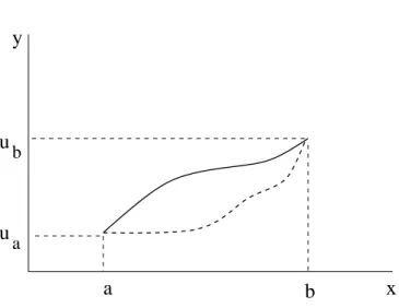
Euler equation. Let u ∈ V be a solution of (P) and assume additionally u∈ C2(a, b), then d dxfu0(x, u(x), u 0(x)) = f u(x, u(x), u0(x)) in (a, b).
Proof. Exercise. Hints: For fixed φ ∈ C2[a, b] with φ(a) = φ(b) = 0 and
real ², |²| < ²0, set g(²) = E(u + ²φ). Since g(0)≤ g(²) it follows g0(0) = 0.
Integration by parts in the formula for g0(0) and the following basic lemma
y
x
b
a
u
u
b aFigure 1.1: Admissible variations
Basic lemma in the calculus of variations. Let h∈ C(a, b) and Z b
a
h(x)φ(x) dx = 0
for all φ∈ C1
0(a, b). Then h(x)≡ 0 on (a, b).
Proof. Assume h(x0) > 0 for an x0 ∈ (a, b), then there is a δ > 0 such that
(x0− δ, x0+ δ)⊂ (a, b) and h(x) ≥ h(x0)/2 on (x0− δ, x0+ δ). Set
φ(x) = ½ ¡ δ2− |x − x 0|2¢2 if x∈ (x0− δ, x0+ δ) 0 if x∈ (a, b) \ [x0− δ, x0+ δ] . Thus φ∈ C1 0(a, b) and Z b a h(x)φ(x) dx≥ h(x0) 2 Z x0+δ x0−δ φ(x) dx > 0,
which is a contradiction to the assumption of the lemma. 2
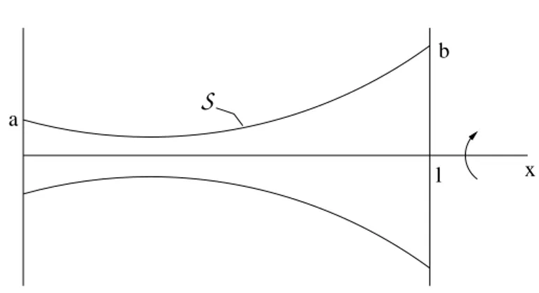
1.2.1 Rotationally symmetric minimal surface
Consider a curve defined by v(x), 0≤ x ≤ l, which satisfies v(x) > 0 on [0, l] and v(0) = a, v(l) = b for given positive a and b, see Figure 1.2. LetS(v)
a
b
l x
S
Figure 1.2: Rotationally symmetric surface
be the surface defined by rotating the curve around the x-axis. The area of this surface is |S(v)| = 2π Z l 0 v(x)p1 + (v0(x))2 dx. Set V ={v ∈ C1[0, l] : v(0) = a, v(l) = b, v(x) > 0 on (a, b)}. Then the variational problem which we have to consider is
min
v∈V |S(v)|.
Solutions of the associated Euler equation are catenoids (= chain curves), see an exercise.
1.2.2 Brachistochrone
In 1696 Johann Bernoulli studied the problem of a brachistochrone to find a curve connecting two points P1 and P2 such that a mass point moves from
P1 to P2 as fast as possible in a downward directed constant gravitional
field, see Figure 1.3. The associated variational problem is here
min (x,y)∈V Z t2 t1 p x0(t)2+ y0(t)2 p y(t)− y1+ k dt ,
where V is the set of C1[t
1, t2] curves defined by (x(t), y(t)), t1 ≤ t ≤ t2, with
x0(t)2+ y0(t)2 6= 0, (x(t1), y(t1)) = P1, (x(t2), y(t2)) = P2 and k := v12/2g,
where v1 is the absolute value of the initial velocity of the mass point, and
y P 1 m P 2 x g
Figure 1.3: Problem of a brachistochrone
and Chapter 3. These functions are solutions of the system of the Euler differential equations associated to the above variational problem.
One arrives at the above functional which we have to minimize since v = q 2g(y− y1) + v12, v = ds/dt, ds = p x1(t)2+ y0(t)2dt and T = Z t2 t1 dt = Z t2 t1 ds v ,
where T is the time which the mass point needs to move from P1 to P2.
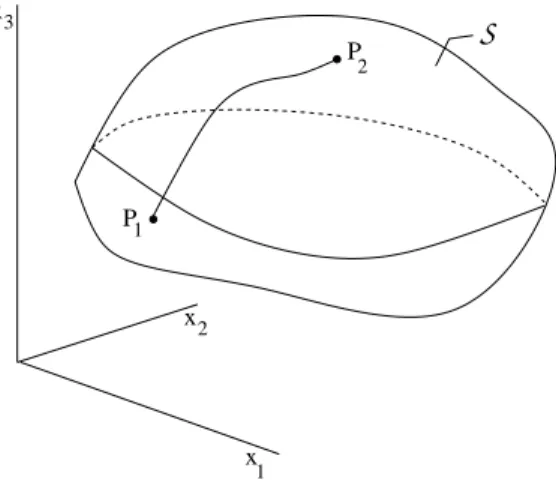
1.2.3 Geodesic curves
Consider a surface S in R3, two points P
1, P2 on S and a curve on S
connecting these points, see Figure 1.4. Suppose that the surfaceS is defined by x = x(v), where x = (x1, x2, x3) and v = (v1, v2) and v ∈ U ⊂ R2.
Consider curves v(t), t1 ≤ t ≤ t2, in U such that v∈ C1[t1, t2] and v10(t)2+
v20(t)2 6= 0 on [t1, t2], and define
V ={v ∈ C1[t1, t2] : x(v(t1)) = P1, x(v(t2)) = P2}.
The length of a curve x(v(t)) for v∈ V is given by L(v) = Z t2 t1 r dx(v(t)) dt · dx(v(t)) dt dt.
Set E = xv1 · xv1, F = xv1 · xv2, G = xv2 · xv2. The functions E, F and G are called coefficients of the first fundamental form of Gauss. Then we get for the length of the cuve under consideration
L(v) = Z t2 t1 q E(v(t))v0 1(t)2+ 2F (v(t))v01(t)v20(t) + G(v(t))v02(t)2 dt
P P 1 2 S x 1 x2 x3
Figure 1.4: Geodesic curves
and the associated variational problem to study is here
min
v∈V L(v).
For examples of surfaces (sphere, ellipsoid) see [9], Part II.
1.2.4 Critical load
Consider the problem of the critical Euler load P for a beam. This value is given by P = min V \{0} a(v, v) b(v, v), where a(u, v) = EI Z l 0 u00(x)v00(x) dx b(u, v) = Z 2 0 u0(x)v0(x) dx and E modulus of elasticity,
I surface moment of inertia, EI is called bending stiffness,
V is the set of admissible deflections defined by the prescribed conditions at the ends of the beam. In the case of a beam simply supported at both ends, see Figure 1.5(a), we have
P (a) (b) P v v l l
Figure 1.5: Euler load of a beam
V ={v ∈ C2[0, l] : v(0) = v(l) = 0}
which leads to the critical value P = EIπ2/l2. If the beam is clamped at the lower end and free (no condition is prescribed) at the upper end, see Figure 1.5(b), then
V ={v ∈ C2[0, l] : v(0) = v0(0) = 0}, and the critical load is here P = EIπ2/(4l2).
Remark. The quotient a(v, v)/b(v, v) is called Rayleigh quotient (Lord Rayleigh, 1842-1919).
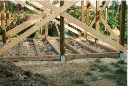
Example: Summer house
As an example we consider a summer house based on columns, see Fig-ure 1.6:
9 columns of pine wood, clamped at the lower end, free at the upper end, 9 cm× 9 cm is the cross section of each column,
2,5 m length of a column,
9 - 16· 109 N m−2 modulus of elasticity, parallel fiber,
0.6 - 1· 109 N m−2 modulus of elasticity, perpendicular fiber,
I = Z Z
Ω
I = 546.75· 10−8m4,
E := 5× 10⁹ N m−2,
P=10792 N, m=1100 kg (g:=9.80665 ms−2),
9 columns: 9900 kg, 18 m2 area of the flat roof, 10 cm wetted snow: 1800 kg.
Figure 1.6: Summer house construction
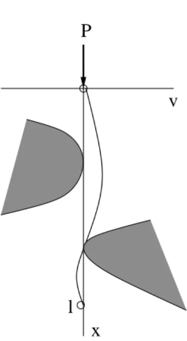
Unilateral buckling
If there are obstacles on both sides, see Figure 1.7, then we have in the case of a beam simply supported at both ends
V ={v ∈ C2[0, l] : v(0) = v(l) = 0 and φ1(x)≤ v(x) ≤ φ2(x) on (0, l)}.
The critical load is here
P = inf
V \{0}
a(v, v) b(v, v).
It can be shown, see [37, 38], that this number P is the lowest point of bifurcation of the eigenvalue variational inequality
v
P
l
x
Figure 1.7: Unilateral beam
A real λ0 is said to be a point of bifurcation of the the above inequality if
there exists a sequence un, un6≡ 0, of solutions with associated eigenvalues
λn such that un→ 0 uniformly on [0, l] and λn→ λ0.
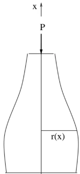
Optimal design of a column
Consider a rotationally symmetric column, see Figure 1.8. Let l be the length of the column,
r(x) radius of the cross section,
I(x) = π(r(x))4/4 surface moment of inertia, ρ constant density of the material,
E modulus of elasticity. Set a(r)(u, v) = Z l 0 r(x)4u00(x)v00(x) dx−4ρ E Z l 0 µZ l x r(t)2dt ¶ u0(x)v0(x) dx b(r)(v, v) = Z l 0 u0(x)v0(x) dx.
Suppose that ρ/E is sufficiently small to avoid that the column is unstable without any load P . If the column is clamped at the lower end and free at
P x
r(x)
Figure 1.8: Optimal design of a column
the upper end, then we set
V ={v ∈ C2[0, l] : v(0) = v0(0) = 0} and consider the Rayleigh quotient
q(r, v) = a(r)(v, v) b(r)(v, v).
We seek an r such that the critical load P (r) = Eπλ(r)/4, where λ(r) = min
v∈V \{0}q(r, v),
approaches its infimum in a given set U of functions, for example
U ={r ∈ C[a, b] : r0 ≤ r(x) ≤ r1, π
Z l 0
r(x)2 dx = M},
where r0, r1 are given positive constants and M is the given volume of the
column. That is, we consider the saddle point problem
max r∈U µ min v∈V \{0}q(r, v) ¶ .
Let (r0, v0) be a solution, then
q(r, v0)≤ q(r0, v0)≤ q(r0, v)
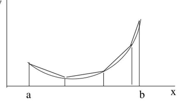
1.2.5 Euler’s polygonal method
Consider the functional
E(v) = Z b a f (x, v(x), v0(x)) dx, where v∈ V with V ={v ∈ C1[a, b] : v(a) = A, v(b) = B} with given A, B. Let
a = x0 < x1 < . . . < xn< xn+1= b
be a subdivision of the interval [a, b]. Then we replace the graph defined by v(x) by the polygon defined by (x0, A), (x1, v1), ... , (xn, vn), (xn+1, B),
where vi = v(xi), see Figure 1.9. Set hi = xi− xi−1 and v = (v1, . . . , vn),
v
x
a
b
Figure 1.9: Polygonal method
and replace the above integral by
e(v) = n+1X i=1 f µ xi, vi, vi− vi−1 hi ¶ hi.
The problem minv∈Rne(v) is an associated finite dimensional problem to minv∈V E(v). Then one shows, under additional assumptions, that the finite
dimensional problem has a solution which converges to a solution to the original problem if n→ ∞.
Remark. The historical notation ”problems with infinitely many variables” for the above problem for the functional E(v) has its origin in Euler’s polyg-onal method.
1.2.6 Optimal control
As an example for problems in optimal control theory we mention here a problem governed by ordinary differential equations. For a given function v(t)∈ U ⊂ Rm, t
0 ≤ t ≤ t1, we consider the boundary value problem
y0(t) = f (t, y(t), v(t)), y(t0) = x0, y(t1) = x1,
where y ∈ Rn, x0, x1 are given, and
f : [t0, t1]× Rn× Rm7→ Rn.
In general, there is no solution of such a problem. Therefore we consider the set of admissible controls Uad defined by the set of piecewise continuous
functions v on [t0, t1] such that there exists a solution of the boundary value
problem. We suppose that this set is not empty. Assume a cost functional is given by E(v) = Z t1 t0 f0(t, y(t)), v(t)) dt, where f0 : [t0, t1]× Rn× Rm7→ R,
v ∈ Uad and y(t) is the solution of the above boundary value problem with
the control v.
The functions f, f0 are assumed to be continuous in (t, y, v) and contin-uously differentiable in (t, y). It is not required that these functions are differentiable with respect to v.
Then the problem of optimal control is
max
v∈Uad E(v).
A piecewise continuous solution u is called optimal control and the solution x of the associated system of boundary value problems is said to be optimal trajectory.
The governing necessary condition for this type of problems is the Pon-tryagin maximum principle, see [48] and Section 3.5.
1.3
Partial differential equations
The same procedure as above applied to the following multiple integral leads to a second-order quasilinear partial differential equation. Set
E(v) = Z Ω F (x, v,∇v) dx, where Ω ⊂ Rn is a domain, x = (x 1, . . . , xn), v = v(x) : Ω 7→ R, and
∇v = (vx1, . . . , vxn). It is assumed that the function F is sufficiently regular in its arguments. For a given function h, defined on ∂Ω, set
V ={v ∈ C1(Ω) : v = h on ∂Ω}.
Euler equation. Let u ∈ V be a solution of (P), and additionally u ∈ C2(Ω), then n X i=1 ∂ ∂xi Fuxi = Fu in Ω.
Proof. Exercise. Hint: Extend the above fundamental lemma of the calculus of variations to the case of multiple integrals. The interval (x0− δ, x0+ δ) in
the definition of φ must be replaced by a ball with center at x0 and radius
δ. 2
1.3.1 Dirichlet integral
In two dimensions the Dirichlet integral is given by
D(v) = Z
Ω
¡
vx2+ vy2¢ dxdy
and the associated Euler equation is the Laplace equation4u = 0 in Ω. Thus, there is natural relationship between the boundary value problem
4u = 0 in Ω, u = h on ∂Ω and the variational problem
min
But these problems are not equivalent in general. It can happen that the boundary value problem has a solution but the variational problem has no solution. For an example see Courant and Hilbert [9], Vol. 1, p. 155, where h is a continuous function and the associated solution u of the boundary value problem has no finite Dirichlet integral.
The problems are equivalent, provided the given boundary value function h is in the class H1/2(∂Ω), see Lions and Magenes [35].
1.3.2 Minimal surface equation
The non-parametric minimal surface problem in two dimensions is to find a minimizer u = u(x1, x2) of the problem
min v∈V Z Ω q 1 + v2 x1 + v 2 x2 dx,
where for a given function h defined on the boundary of the domain Ω V ={v ∈ C1(Ω) : v = h on ∂Ω}.
Suppose that the minimizer satisfies the regularity assumption u∈ C2(Ω),
S
Ω
Figure 1.10: Comparison surface
then u is a solution of the minimal surface equation (Euler equation) in Ω ∂ ∂x1 Ã ux1 p 1 +|∇u|2 ! + ∂ ∂x2 Ã ux2 p 1 +|∇u|2 ! = 0.
In fact, the additional assumption u∈ C2(Ω) is superfluous since it follows
from regularity considerations for quasilinear elliptic equations of second order, see for example Gilbarg and Trudinger [20].
Let Ω = R2. Each linear function is a solution of the minimal surface equation. It was shown by Bernstein [4] that there are no other solutions of the minimal surface equation. This is true also for higher dimensions n≤ 7, see Simons [56]. If n≥ 8, then there exists also other solutions which define cones, see Bombieri, De Giorgi and Giusti [7].
The linearized minimal surface equation over u≡ 0 is the Laplace equa-tion 4u = 0. In R2 linear functions are solutions but also many other
functions in contrast to the minimal surface equation. This striking differ-ence is caused by the strong nonlinearity of the minimal surface equation.
More general minimal surfaces are described by using parametric rep-resentations. An example is shown in Figure 1.111. See [52], pp. 62, for example, for rotationally symmetric minimal surfaces, and [47, 12, 13] for more general surfaces. Suppose that the surface S is defined by y = y(v),
Figure 1.11: Rotationally symmetric minimal surface
where y = (y1, y2, y3) and v = (v1, v2) and v ∈ U ⊂ R2. The area of the
surfaceS is given by |S(y)| = Z U p EG− F2 dv,
where E = yv1 · yv1, F = yv1 · yv2, G = yv2 · yv2 are the coefficients of the first fundamental form of Gauss. Then an associated variational problem is
min
y∈V |S(y)|,
where V is a given set of comparison surfaces which is defined, for example, by the condition that y(∂U ) ⊂ Γ, where Γ is a given curve in R3, see Figure 1.12. Set V = C1(Ω) and
x
1
x2 x3
S
Figure 1.12: Minimal surface spanned between two rings
E(v) = Z Ω F (x, v,∇v) dx − Z ∂Ω g(x, v) ds,
where F and g are given sufficiently regular functions and Ω ⊂ Rn is a
bounded and sufficiently regular domain. Assume u is a minimizer of E(v) in V , that is,
u∈ V : E(u) ≤ E(v) for all v ∈ V, then Z Ω ¡Xn i=1 Fuxi(x, u,∇u)φxi + Fu(x, u,∇u)φ ¢ dx − Z ∂Ω gu(x, u)φ ds = 0
for all φ∈ C1(Ω). Assume additionally that u∈ C2(Ω), then u is a solution
of the Neumann type boundary value problem
n X i=1 ∂ ∂xi Fuxi = Fu in Ω n X i=1 Fuxiνi = gu on ∂Ω,
where ν = (ν1, . . . , νn) is the exterior unit normal at the boundary ∂Ω. This
follows after integration by parts from the basic lemma of the calculus of variations. Set E(v) = 1 2 Z Ω |∇v| 2 dx−Z ∂Ω h(x)v ds,
then the associated boundary value problem is
4u = 0 in Ω ∂u
∂ν = h on ∂Ω.
1.3.3 Capillary equation
Let Ω⊂ R2 and set
E(v) = Z Ω p 1 +|∇v|2 dx + κ 2 Z Ω v2 dx− cos γ Z ∂Ω v ds.
Here is κ a positive constant (capillarity constant) and γ is the (constant) boundary contact angle, that is, the angle between the container wall and the capillary surface, defined by v = v(x1, x2), at the boundary. Then the
related boundary value problem is
div (T u) = κu in Ω ν· T u = cos γ on ∂Ω, where we use the abbreviation
T u = p ∇u 1 +|∇u|2,
div (T u) is the left hand side of the minimal surface equation and it is twice the mean curvature of the surface defined by z = u(x1, x2), see an exercise.
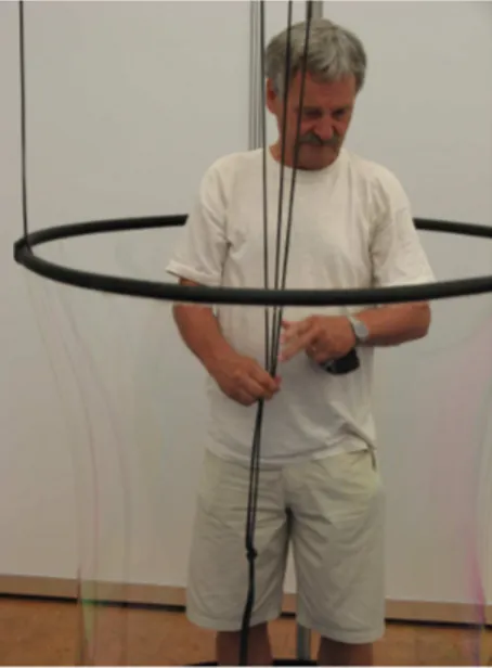
The above problem describes the ascent of a liquid, water for example, in a vertical cylinder with constant cross section Ω. It is assumed that the gravity is directed downwards in the direction of the negative x3 axis.
Figure 1.13 showsthat liquid can rise along a vertical wedge. This is a conse-quence of the strong nonlinearity of the underlying equations, see Finn [16]. This photo was taken from [42].
Figure 1.13: Ascent of liquid in a wedge
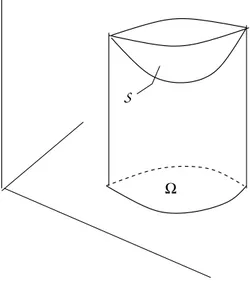
The above problem is a special case (graph solution) of the following problem. Consider a container partially filled with a liquid, see Figure 1.14. Suppose that the associate energy functional is given by
E(S) = σ|S| − σβ|W (S)| + Z
Ωl(S)
Y ρ dx,
where
Y potential energy per unit mass, for example Y = gx3, g = const.≥ 0,
ρ local density,
σ surface tension, σ = const. > 0,
β (relative) adhesion coefficient between the fluid and the container wall, W wetted part of the container wall,
Ωl domain occupied by the liquid.
Additionally we have for given volume V of the liquid the constraint
Ω Ω Ω l v s
S
liquid vapour (solid) x 3 gFigure 1.14: Liquid in a container
It turns out that a minimizerS0 of the energy functional under the volume
constraint satisfies, see [16],
2σH = λ + gρx3 on S0
cos γ = β on ∂S0,
where H is the mean curvature ofS0 and γ is the angle between the surface
S0 and the container wall at ∂S0.
Remark. The term−σβ|W | in the above energy functional is called wetting energy.
Liquid can pilled up on a glass, see Figure 1.15. This picture was taken from [42]. Here the capillary surface S satisfies a variational inequality at ∂S where S meets the container wall along an edge, see [41].
1.3.4 Liquid layers
Porous materials have a large amount of cavities different in size and geom-etry. Such materials swell and shrink in dependence on air humidity. Here we consider an isolated cavity, see [54] for some cavities of special geometry. Let Ωs∈ R3 be a domain occupied by homogeneous solid material. The
question is whether or not liquid layers Ωl on Ωs are stable, where Ωv is
the domain filled with vapour and S is the capillary surface which is the interface between liquid and vapour, see Figure 1.16.
N
Ω
sΩ
vΩ
l liquid vapoursolid
S
Figure 1.16: Liquid layer in a pore
Let
E(S) = σ|S| + w(S) − µ|Dl(S)| (1.1)
be the energy (grand canonical potential) of the problem, where
σ surface tension, |S|, |Ωl(S)| denote the area resp. volume of S, Ωl(S),
w(S) = − Z
Ωv(S)
F (x) dx , (1.2)
is the disjoining pressure potential, where
F (x) = c Z
Ωs dy
|x − y|p . (1.3)
Here is c a negative constant, p > 4 a positive constant (p = 6 for nitrogen) and x∈ R3\ Ω
Ωs with its boundary ∂Ωs. Finally, set
µ = ρkT ln(X) , where
ρ density of the liquid, k Boltzmann constant, T absolute temperature,
X reduced (constant) vapour pressure, 0 < X < 1.
More precisely, ρ is the difference between the number densities of the liquid and the vapour phase. However, since in most practical cases the vapour density is rather small, ρ can be replaced by the density of the liquid phase.
The above negative constant is given by c = H/π2, where H is the
Hamaker constant, see [25], p. 177. For a liquid nitrogen film on quartz one has aboutH = −10−20N m.
Suppose thatS0 defines a local minimum of the energy functional, then
−2σH + F − µ = 0 on S0 , (1.4)
where H is the mean curvature ofS0.
A surfaceS0 which satisfies (1.4) is said to be an equilibrium state. An
existing equilibrium stateS0 is said to be stable by definition if
· d2 d²2E(S(²)) ¸ ²=0 > 0
for all ζ not identically zero, where S(²) is an appropriate one-parameter family of comparison surfaces.
This inequality implies that
−2(2H2− K) + 1 σ
∂F
∂N > 0 onS0, (1.5)
where K is the Gauss curvature of the capillary surfaceS0, see Blaschke [5], p. 58,
for the definition of K.
1.3.5 Extremal property of an eigenvalue
Let Ω⊂ R2 be a bounded and connected domain. Consider the eigenvalue
problem
−4u = λu in Ω u = 0 on ∂Ω.
It is known that the lowest eigenvalue λ1(Ω) is positive, it is a simple
eigen-value and the associated eigenfunction has no zero in Ω. Let V be a set of sufficiently regular domains Ω with prescribed area |Ω|. Then we consider the problem
min
Ω∈V λ1(Ω).
The solution of this problem is a disk BR, R =
p
|Ω|/π, and the solution is uniquely determined.
1.3.6 Isoperimetric problems
Let V be a set of all sufficiently regular bounded and connected domains Ω⊂ R2 with prescribed length |∂Ω| of the boundary. Then we consider the problem
max
Ω∈V |Ω|.
The solution of this problem is a disk BR, R =|∂Ω|/(2π), and the solution
is uniquely determined. This result follows by Steiner’s symmetrization, see [5], for example. From this method it follows that
|∂Ω|2− 4π|Ω| > 0 if Ω is a domain different from a disk.
Remark. Such an isoperimetric inequality follows also by using the
in-equality Z R2 |u| dx ≤ 1 4π Z R2 |∇u| 2 dx for all u ∈ C1
0(R2). After an appropriate definition of the integral on the
right hand side this inequality holds for functions from the Sobolev space H01(Ω), see [1], or from the class BV (Ω), which are the functions of bounded variation, see [15]. The set of characteristic functions for sufficiently regular domains is contained in BV (Ω) and the square root of the integral of the right hand defines the perimeter of Ω. Set
u = χΩ = ½ 1 : x∈ Ω 0 : x6∈ Ω then |Ω| ≤ 1 4π|∂Ω| 2.
The associated problem in R3 is max
Ω∈V |Ω|,
where V is the set of all sufficiently regular bounded and connected domains Ω⊂ R3 with prescribed perimeter |∂Ω|. The solution of this problem is a
ball BR, R =
p
|∂Ω|/(4π), and the solution is uniquely determined, see [5], for example, where it is shown that the isoperimetric inequality
|∂Ω|3− 36π|Ω|2 ≥ 0
1.4
Exercises
1. Let V ⊂ Rn be nonempty, closed and bounded and f : V 7→ R lower
semicontinuous on V . Show that there exists an x ∈ V such that f (x)≤ f(y) for all y ∈ V .
Hint: f : V 7→ Rn is called lower semicontinuous on V if for every
sequence xk → x, xk, x∈ V , it follows that
lim inf
k→∞ f (x
k)≥ f(x).
2. Let V ⊂ Rnbe the closure of a convex domain and assume f : V 7→ R
is in C1(Rn). Suppose that x∈ V satisfies f(x) ≤ f(y) for all y ∈ V . Prove
(i) h∇f(x), y − xi ≥ 0 for all y ∈ V ,
(ii) ∇f(x) = 0 if x is an interior point of V .
3. Let A and B be real and symmetric matrices with n rows (and n columns). Suppose that B is positive, i. e., hBy, yi > 0 for all y ∈ Rn\ {0}.
(i) Show that there exists a solution x of the problem
min
y∈Rn\{0}
hAy, yi hBy, yi.
(ii) Show that Ax = λBx, where λ =hAx, xi/hBx, xi.
Hint: (a) Show that there is a positive constant such that hBy, yi ≥ chy, yi for all y ∈ Rn.
(b) Show that there exists a solution x of the problem minyhAy, yi,
where hBy, yi = 1. (c) Consider the function
g(²) = hA(x + ²y), x + ²yi hB(x + ²y, x + ²yi,
where |²| < ²0, ²0 sufficiently small, and use that g(0)≤ g(²).
4. Let A and B satisfy the assumption of the previous exercise. Let C be a closed convex nonempty cone in Rn with vertex at the origin.
Assume C 6= {0}.
(i) Show that there exists a solution x of the problem
min
y∈C\{0}
hAy, yi hBy, yi.
(ii) Show that x is a solution of
x∈ C : hAx, y − xi ≥ λhx, y − xi for all y ∈ C, where λ =hAx, xi/hBx, xi.
Hint: To show (ii) consider for x y ∈ C the function g(²) = hA(x + ²(y − x)), x + ²(y − x)i
hB(x + ²(y − x)), x + ²(y − x)i,
where 0 < ² < ²0, ²0 sufficiently small, and use g(0) ≤ g(²) which
implies that g0(0)≥ 0.
5. Let A be real matrix with n rows and n columns, and let C ⊂ Rn be a nonempty closed and convex cone with vertex at the origin. Show that
x∈ C : hAx, y − xi ≥ 0 for all y ∈ C is equivalent to
hAx, xi = 0 and hAx, yi ≥ 0 for all y ∈ C. Hint: 2x, x + y ∈ C if x, y ∈ C.
6. R. Courant. Show that
E(v) := Z 1
0
¡
1 + (v0(x))2¢1/4dx does not achieve its infimum in the class of functions
V ={v ∈ C[0, 1] : v piecewise C1, v(0) = 1, v(1) = 0}, i. e., there is no u∈ V such that E(u) ≤ E(v) for all v ∈ V . Hint: Consider the family of functions
v(²; x) = ½
(²− x)/² : 0 ≤ x ≤ ² < 1 0 : x > ²
7. K. Weierstraß, 1895. Show that
E(v) = Z 1
−1
does not achieve its infimum in the class of functions V =©v∈ C1[−1, 1] : v(−1) = a, v(1) = bª, where a6= b. Hint: v(x; ²) = a + b 2 + b− a 2 arctan(x/²) arctan(1/²)
defines a minimal sequence, i. e., lim²→0E(v(²)) = infv∈V E(v).
8. Set
g(²) := Z b
a
f (x, u(x) + ²φ(x), u0(x) + ²φ0(x)) dx,
where ²,|²| < ²0, is a real parameter, f (x, z, p) in C2 in his arguments
and u, φ∈ C1[a, b]. Calculate g0(0) and g00(0).
9. Find all C2-solutions u = u(x) of
d dxfu0 = fu, if f =p1 + (u0)2. 10. Set E(v) = Z 1 0 ¡ v2(x) + xv0(x)¢ dx and V ={v ∈ C1[0, 1] : v(0) = 0, v(1) = 1}. Show that minv∈V E(v) has no solution.
11. Is there a solution of minv∈V E(v), where V = C[0, 1] and
E(v) = Z 1 0 ÃZ v(x) 0 (1 + ζ2) dζ ! dx ?
12. Let u ∈ C2(a, b) be a solution of Euler’s differential equation. Show
that u0fu0 − f ≡ const., provided that f = f(u, u0), i. e., f depends not explicitly on x.
13. Consider the problem of rotationally symmetric surfaces minv∈V |S(v)|, where |S(v)| = 2π Z l 0 v(x)p1 + (v0(x))2 dx and V ={v ∈ C1[0, l] : v(0) = a, v(l) = b, v(x) > 0 on (a, b)}. Find C2(0, l)-solutions of the associated Euler equation.
Hint: Solutions are catenoids (chain curves, in German: Kettenlinien). 14. Find solutions of Euler’s differential equation to the Brachistochrone
problem minv∈VE(v), where
V ={v ∈ C[0, a]∩C2(0, a] : v(0) = 0, v(a) = A, v(x) > 0 if x∈ (0, a]}, that is, we consider here as comparison functions graphs over the x-axis, and E(v) = Z a 0 √ 1 + v02 √ v dx .
Hint: (i) Euler’s equation implies that
y(1 + y02) = α2, y = y(x),
with a constant α. (ii) Substitution
y = c
2(1− cos u), u = u(x),
implies that x = x(u), y = y(u) define cycloids (in German: Rollkur-ven).
15. Prove the basic lemma in the calculus of variations: Let Ω⊂ Rn be a domain and f ∈ C(Ω) such that
Z
Ω
f (x)h(x) dx = 0
for all h∈ C1
0(Ω). Then f ≡ 0 in Ω.
16. Write the minimal surface equation as a quasilinear equation of second order.
17. Prove that a minimizer in C1(Ω) of E(v) = Z Ω F (x, v,∇v) dx − Z ∂Ω g(v, v) ds,
is a solution of the boundary value problem, provided that additionally u∈ C2(Ω), n X i=1 ∂ ∂xi Fuxi = Fu in Ω n X i=1 Fuxiνi = gu on ∂Ω,
Functions of n variables
In this chapter, with only few exceptions, the normed space will be the n-dimensional Euclidean space Rn. Let f be a real function defined on a nonempty subset X ⊆ Rn. In the conditions below where derivatives occur,
we assume that f ∈ C1 or f ∈ C2 on an open set X⊆ Rn.
2.1
Optima, tangent cones
Let f be a real-valued functional defined on a nonempty subset V ⊆ X. Definition. We say that an element x ∈ V defines a global minimum of f in V , if
f (x)≤ f(y) for all y∈ V,
and we say that x∈ V defines a strict global minimum, if the strict inequal-ity holds for all y ∈ V, y 6= x.
For a ρ > 0 we define a ball Bρ(x) with radius ρ and center x:
Bρ(x) ={y ∈ Rn; ||y − x|| < ρ},
where ||y − x|| denotes the Euclidean norm of the vector x − y. We always assume that x∈ V is not isolated i. e., we assume that V ∩ Bρ(x)6= {x} for
all ρ > 0.
Definition. We say that an element x∈ V defines a local minimum of f in V if there exists a ρ > 0 such that
f (x)≤ f(y) for all y ∈ V ∩ Bρ(x),
and we say that x∈ V defines a strict local minimum if the strict inequality holds for all y∈ V ∩ Bρ(x), y6= x.
That is, a global minimum is a local minimum. By reversing the direc-tions of the inequality signs in the above definidirec-tions, we obtain definidirec-tions of global maximum, strict global maximum, local maximum and strict local maximum. An optimum is a minimum or a maximum and a local optimum is a local minimum or a local maximum. If x defines a local maximum etc. of f , then x defines a local minimum etc. of−f, i. e., we can restrict ourselves to the consideration of minima.
In the important case that V and f are convex, then each local minimum defines also a global minimum. These assumptions are satisfied in many applications to problems in microeconomy.
Definition. A subset V ⊆ X is said to be convex if for any two vectors x, y∈ V the inclusion λx + (1 − λ)y ∈ V holds for all 0 ≤ λ ≤ 1.
Definition. We say that a functional f defined on a convex subset V ⊆ X is convex if
f (λx + (1− λ)y) ≤ λf(x) + (1 − λ)f(y)
for all x, y∈ V and for all 0 ≤ λ ≤ 1, and f is strictly convex if the strict inequality holds for all x, y∈ V , x 6= y, and for all λ, 0 < λ < 1.
Theorem 2.1.1. If f is a convex functional on a convex set V ⊆ X, then any local minimum of f in V is a global minimum of f in V .
Proof. Suppose that x is no global minimum, then there exists an x1 ∈ V such that f (x1) < f (x). Set y(λ) = λx1+ (1− λ)x, 0 < λ < 1, then
f (y(λ))≤ λf(x1) + (1− λ)f(x) < λf(x) + (1 − λ)f(x) = f(x). For each given ρ > 0 there exists a λ = λ(ρ) such that y(λ) ∈ Bρ(x) and
f (y(λ)) < f (x). This is a contradiction to the assumption. 2
Concerning the uniqueness of minimizers one has the following result.
Theorem 2.1.2. If f is a strictly convex functional on a convex set V ⊆ X, then a minimum (local or global) is unique.
see Theorem 2.1.1. Assume x1 6= x2, then for 0 < λ < 1
f (λx1+ (1− λ)x2) < λf (x1) + (1− λ)f(x2) = f (x1) = f (x2).
This is a contradiction to the assumption that x1, x2 define global minima. 2
Theorem 2.1.3. a) If f is a convex function and V ⊂ X a convex set, then the set of minimizers is convex.
b) If f is concave, V ⊂ X convex, then the set of maximizers is convex. Proof. Exercise.
In the following we use for (fx1(x), . . . , fxn) the abbreviations f
0(x),∇f(x)
or Df (x).
Theorem 2.1.4. Suppose that V ⊂ X is convex. Then f is convex on V if and only if
f (y)− f(x) ≥ hf0(x), y− xi for all x, y ∈ V.
Proof. (i) Assume f is convex. Then for 0≤ λ ≤ 1 we have f (λy + (1− λ)x) ≤ λf(y) + (1 − λ)f(x)
f (x + λ(y− x)) ≤ f(x) + λ(f(y) − f(x)) f (x) + λhf0(x), y− xi + o(λ) ≤ f(x) + λ(f(y) − f(x)), which implies that
hf0(x), y− xi ≤ f(y) − f(x). (ii) Set for x, y∈ V and 0 < λ < 1
x1:= (1− λ)y + λx and h := y − x1. Then
x = x1−1− λ λ h.
Since we suppose that the inequality of the theorem holds, we have f (y)− f(x1) ≥ hf0(x1), y− x1i = hf0(x1), hi
f (x)− f(x1) ≥ hf0(x1), x− x1i = −1− λ λ hf
After multiplying the first inequality with (1−λ)/λ we add both inequalities and get 1− λ λ f (y)− 1− λ λ f (x 1) + f (x)− f(x1) ≥ 0 (1− λ)f(y) + λf(x) − (1 − λ)f(x1)− λf(x1) ≥ 0. Thus (1− λ)f(y) + λf(x) ≥ f(x1)≡ f((1 − λ)y − λx) for all 0 < λ < 1. 2
Remark. The inequality of the theorem says that the surfaceS defined by z = f (y) is above of the tangent plane Txdefined by z =hf0(x), y−xi+f(x),
see Figure 2.1 for the case n = 1.
x y
z
Tx
S
Figure 2.1: Figure to Theorem 2.1.4
The following definition of a local tangent cone is fundamental for our considerations, particularly for the study of necessary conditions in con-strained optimization. The tangent cone plays the role of the tangent plane in unconstrained optimization.
Definition. A nonempty subset C⊆ Rnis said to be a cone with vertex at
z∈ Rn, if y∈ C implies that z + t(y − z) ∈ C for each t > 0.
Definition. For given x∈ V we define the local tangent cone of V at x by T (V, x) = {w ∈ Rn: there exist sequences xk ∈ V, tk∈ R, tk > 0,
such that xk→ x and tk(xk− x) → w as k → ∞}.
This definition implies immediately
T(V,x) V
x
Figure 2.2: Tangent cone
Corollaries. (i) The set T (V, x) is a cone with vertex at zero.
(ii) A vector x∈ V is not isolated if and only if T (V, x) 6= {0}. (iii) Suppose that w 6= 0, then tk→ ∞.
(iv) T (V, x) is closed.
(v) T (V, x) is convex if V is convex.
In the following the Hesse matrix (fxixj)
n
i,j=1is also denoted by f00(x), fxx(x)
or D2f (x).
Theorem 2.1.5. Suppose that V ⊂ Rn is nonempty and convex. Then
(i) If f is convex on V , then the Hesse matrix f00(x), x ∈ V , is positive semidefinite on T (V, x). That is,
for all x∈ V and for all w ∈ T (V, x).
(ii) Assume the Hesse matrix f00(x), x ∈ V , is positive semidefinite on Y = V − V , the set of all x − y where x, y ∈ V . Then f is convex on V . Proof. (i) Assume f is convex on V . Then for all x, y ∈ V , see Theo-rem 2.1.4, f (y)− f(x) ≥ hf0(x), y− xi. Thus hf0(x), y− xi + 1 2hf 00(x)(y − x), y − xi + o(||y − x||2) ≥ hf0(x), y− xi hf00(x)(y− x), y − xi + ||y − x||2η(||y − x||) ≥ 0,
where limt→0η(t) = 0. Suppose that w ∈ T (V, x) and that tk, xk → x are
associated sequences, i. e., xk∈ V , tk> 0 and
wk:= tk(xk− x) → w.
Then
hf00(x)wk, wki + ||wk||2η(||xk− x||) ≥ 0, which implies that
hf00(x)w, wi ≥ 0. (ii) Since
f (y)− f(x) − hf0(x), y− xi = 1 2hf
00(x + δ(y− x))(y − x), y − xi,
where 0 < δ < 1, and the right hand side is nonnegative, it follows from
2.1.1 Exercises
1. Assume V ⊂ Rn is a convex set. Show that Y = V − V := {x − y :
x, y∈ V } is a convex set in Rn, 0∈ Y and if y ∈ Y then −y ∈ Y . 2. Prove Theorem 2.1.3.
3. Show that T (V, x) is a cone with vertex at zero.
4. Assume V ⊆ Rn. Show that T (V, x)6= {0} if and only if x ∈ V is not
isolated.
5. Show that T (V, x) is closed.
6. Show that T (V, x) is convex if V is a convex set. 7. Suppose that V is convex. Show that
T (V, x) = {w ∈ Rn; there exist sequences xk∈ V, tk∈ R, tk> 0,
such that tk(xk− x) → w as k → ∞}.
8. Assume if w ∈ T (V, x), w 6= 0. Then tk → ∞, where tk are the reals
from the definition of the local tangent cone.
9. Let p∈ V ⊂ Rn and|p|2= p21+ . . . + p2n. Prove that f (p) =p1 +|p|2
is convex on convex sets V .
Hint: Show that the Hesse matrix f00(p) is nonnegative by calculating
hf00(p)ζ, ζi, where ζ ∈ Rn.
10. Suppose that f00(x), x ∈ V , is positive on (V − V ) \ {0}. Show that f (x) is strictly convex on V .
Hint: (i) Show that f (y)−f(x) > hf0(x), y−xi for all x, y ∈ V , x 6= y.
(ii) Then show that f is strictly convex by adapting part (ii) of the proof of Theorem 2.1.4.
11. Let V ⊂ X be a nonempty convex subset of a linear space X and f : V 7→ R. Show that f is convex on V if and only if Φ(t) := f (x + t(y− x)) is convex on t ∈ [0, 1] for all (fixed) x, y ∈ V .
Hint: To see that Φ is convex if f is convex we have to show Φ(λs1+ (1− λ)s2))≤ λΦ(s1) + (1− λ)Φ(s2),
0≤ λ ≤ 1, si∈ [0, 1]. Set τ = λs1+ (1− λ)s2), then
Φ(τ ) = f (x + τ (y− x)) and
x + τ (y− x) = x + (λs1+ (1− λ)s2) (y− x)
2.2
Necessary conditions
The proof of the following necessary condition follows from assumption f ∈ C1(X) and the definition of the tangent cone.
We recall that f is said to be differentiable at x∈ X ⊂ Rn, X open, if all partial derivatives exist at x. In contrast to the case n = 1 it does not follow that f is continuous at x if f is differentiable at that point.
Definition. f is called totally differentiable at x if there exists an a ∈ Rn
such that
f (y) = f (x) +ha, y − xi + o(||x − y||) as y → x.
We recall that
(1) If f is totally differentiable at x, then f is differentiable at x and a = f0(x).
(2) If f ∈ C1(Bρ), then f is totally differentiable at every x∈ Bρ.
(3) Rademacher’s Theorem. If f is locally Lipschitz continuous in Bρ, then
f is totally differentiable almost everywhere in Bρ, i. e., up to a set of
Lebesgue measure zero.
For a proof of Rademacher’s Theorem see [15], pp. 81, for example.
Theorem 2.2.1 (Necessary condition of first order). Suppose that f ∈ C1(X) and that x defines a local minimum of f in V . Then
hf0(x), wi ≥ 0 for all w ∈ T (V, x).
Proof. Let tk, xk be associated sequences to w ∈ T (V, x). Then, since x
defines a local minimum, it follows
0≤ f(xk)− f(x) = hf0(x), xk− xi + o(||xk− x||), which implies that
where limt→0η(t) = 0. Letting n → ∞ we obtain the necessary condition.
2
Corollary. Suppose that V is convex, then the necessary condition of The-orem 1.1.1 is equivalent to
hf0(x), y− xi ≥ 0 for all y ∈ V.
Proof. From the definition of the tangent cone it follows that the corollary implies Theorem 2.2.1. On the other hand, fix y ∈ V and define xk :=
(1−λk)y+λkx, λk∈ (0, 1), λk→ 1. Then xk ∈ V , (1−λk)−1(xk−x) = y−x.
That is, y− x ∈ T (V, x). 2
The variational inequality above is equivalent to a fixed point equation, see Theorem 2.2.2 below.
Let pV(z) be the projection of z∈ H, where H is a real Hilbert space, onto
a nonempty closed convex subset V ⊆ H, see Section 2.6.3 of the appendix. We have w = pV(z) if and only if
hpV(z)− z, y − pV(z)i ≥ 0 for all y ∈ V. (2.1)
Theorem 2.2.2 (Equivalence of a variational inequality to an equation). Suppose that V is a closed convex and nonempty subset of a real Hilbert space H and F a mapping from V into H. Then the variational inequality
x∈ V : hF (x), y − xi ≥ 0 for all y ∈ V. is equivalent to the fixed point equation
x = pV(x− qF (x)) ,
where 0 < q <∞ is an arbitrary fixed constant.
Proof. Set z = x− qF (x) in (2.1). If x = pV(x− qF (x)) then the variational
inequality follows. On the other hand, the variational inequality x∈ V : hx − (x − qF (x)), y − xi ≥ 0 for all y ∈ V
implies that the fixed point equation holds and the above theorem is shown. 2
Remark. This equivalence of a variational inequality with a fixed point equation suggests a simple numerical procedure to calculate solutions of variational inequalities: xk+1 := p
V(xk− qF (xk)). Then the hope is that
the sequence xk converges if 0 < q < 1 is chosen appropriately. In these notes we do not consider the problem of convergence of this or of related numerical procedures. This projection-iteration method runs quite well in some examples, see [51], and exercises in Section 2.5.
In generalization to the necessary condition of second order in the un-constrained case, hf00(x)h, hi ≥ 0 for all h ∈ Rn, we have a corresponding
result in the constrained case.
Theorem 2.2.3 (Necessary condition of second order). Suppose that f ∈ C2(X) and that x defines a local minimum of f in V . Then for each w ∈ T (V, x) and every associated sequences tk, xk the inequality
0≤ lim inf k→∞ tkhf 0(x), wki +1 2hf 00(x)w, wi holds, where wk:= tk(xk− x). Proof. From f (x) ≤ f(xk) = f (x) +hf0(x), xk− xi + 1 2hf 00(x)(xk− x), xk− xi +||xk− x||2η(||xk− x||), where limt→0η(t) = 0, we obtain
0 ≤ tkhf0(x), wki +
1 2hf
00(x)wk, wki + ||wk||2η(||xk− x||).
By taking lim inf the assertion follows. 2
In the next sections we will exploit the explicit nature of the subset V . When the side conditions which define V are equations, then we obtain under an additional assumption from the necessary condition of first order the classical Lagrange multiplier rule.
2.2.1 Equality constraints
Here we suppose that the subset V is defined by
Let gj ∈ C1(Rn), w∈ T (V, x) and tk, xk associated sequences to w. Then
0 = gj(xk)− gj(x) =hg0j(x), xk− xi + o(||xk− x||),
and from the definition of the local tangent cone it follows for each j that
hg0j(x), wi = 0 for all w ∈ T (V, x). (2.2)
Set Y = span{g0
1(x), . . . , g0m(x)} and let Rn= Y⊕Y⊥be the orthogonal
decomposition with respect to the standard Euclidean scalar productha, bi. We recall that dim Y⊥= n− k if dim Y = k.
Equations (2.2) imply immediately that T (V, x)⊆ Y⊥. Under an
addi-tional assumption we have equality.
Lemma 2.2.1. Suppose that dim Y = m (maximal rank condition), then T (V, x) = Y⊥.
Proof. It remains to show that Y⊥ ⊆ T (V, x). Suppose that z ∈ Y⊥, 0 < ²≤ ²0, ²0 sufficiently small. Then we look for solutions y = o(²), depending
on the fixed z, of the system gj(x + ²z + y) = 0, j = 1, . . . , m. Since z∈ Y⊥
and the maximal rank condition is satisfied, we obtain the existence of a y = o(²) as ² → 0 from the implicit function theorem. That is, we have x(²) := x + ²z + y∈ V , where y = o(²). This implies that z ∈ T (V, x) since x(²)→ x, x(²), x ∈ V and ²−1(x(²)− x) → z as ² → 0.
2
From this lemma follows the simplest version of the Lagrange multiplier rule as a necessary condition of first order.
Theorem 2.2.4 (Lagrange multiplier rule, equality constraints). Suppose that x defines a local minimum of f in V and that the maximal rank con-dition of Lemma 2.1.1 is satisfied. Then there exists uniquely determined λj ∈ R, such that f0(x) + m X j=1 λjgj0(x) = 0.
Proof. From the necessary conditionhf0(x), wi ≥ 0 for all w ∈ T (V, x) and
from Lemma 2.2.1 it follows thathf0(x), wi = 0 for all w ∈ Y⊥ since Y⊥ is
a linear space. This equation implies that
Uniqueness of the multipliers follow from the maximal rank condition. 2
There is a necessary condition of second order linked with a Lagrange func-tion L(x, λ) defined by L(x, λ) = f (x) + m X j=1 λjgj(x).
Moreover, under an additional assumption the sequence tkhf0(x), wki, where
wk := tk(xk−x), is convergent, and the limit is independent of the sequences
xk, t
k associated to a given w∈ T (V, x).
We will use the following abbreviations:
L0(x, λ) := f0(x) + m X j=1 λjgj0(x) and L00(x, λ) := f00(x) + m X j=1 λjg00j(x).
Theorem 2.2.5 (Necessary condition of second order, equality constraints). Suppose that f, gj ∈ C2(Rn) and that the maximal rank condition of Lemma 2.2.1
is satisfied. Let x be a local minimizer of f in V and let λ = (λ1, . . . , λm)
be the (uniquely determined) Lagrange multipliers of Theorem 2.2.4 Then (i) hL00(x, λ)z, zi ≥ 0 for all z ∈ Y⊥ (≡ T (V, x)),
(ii) lim k→∞tkhf 0(x), wki =1 2 m X j=1 λjhg00j(x)w, wi, wk:= tk(xk− x),
for all w∈ T (V, x) and for all associated sequences xk, tk
to w ∈ T (V, x) (≡ Y⊥).
Proof. (i) For given z ∈ Y⊥, ||z|| = 1, and 0 < ² ≤ ²
0, ²0 > 0 sufficiently
small, there is a y = o(²) such that gj(x + ²z + y) = 0, j = 1, . . . , m, which
follows from the maximal rank condition and the implicit function theorem. Then f (x + ²z + y) = L(x + ²z + y, λ) = L(x, λ) +hL0(x, λ), ²z + yi +1 2hL 00(x, λ)(²z + y), ²z + yi + o(²2) = f (x) +1 2hL 00(x, λ)(²z + y), ²z + yi + o(²2),
since L0(x, λ) = 0 and x satisfies the side conditions. Hence, since f (x) ≤ f (x + ²z + y), it follows thathL00(x, λ)z, zi ≥ 0.
(ii) Suppose that xk∈ V, tk> 0, such that wk:= tk(xk− x) → w. Then
L(xk, λ) ≡ f(xk) + m X j=1 λjgj(xk) = L(x, λ) + 1 2hL 00(x, λ)(xk− x), xk− xi + o(||xk− x||2). That is, f (xk)− f(x) = 1 2hL 00(x, λ)(xk− x), xk− xi + o(||xk− x||2).
On the other hand,
f (xk)− f(x) = hf0(x), xk− xi + 1 2hf 00(x)(xk− x), xk− xi + o(||xk− x||2). Consequently hf0(x), xk− xi = 1 2 m X j=1 λjhgj00(x)(xk− x, xk− xi + o(||xk− x||2),
which implies (ii) of the theorem. 2
2.2.2 Inequality constraints
We define two index sets by I ={1, . . . , m} and E = {m + 1, . . . , m + p} for integers m≥ 1 and p ≥ 0. If p = 0 then we set E = ∅, the empty set. In this section we assume that the subset V is given by
V ={y ∈ Rn; gj(y)≤ 0 for each j ∈ I and gj(y) = 0 for each j∈ E}
and that gj ∈ C1(Rn) for each j ∈ I ∪ E. Let x ∈ V be a local minimizer
of f in V and let I0 ⊆ I be the subset of I where the inequality constraints
are active, that is, I0 ={j ∈ I; gj(x) = 0}. Let w ∈ T (V, x) and xk, tk are
associated sequences to w, then for k≥ k0, k0 sufficiently large, we have for
each j∈ I0
It follows that for each j∈ I0 hgj0(x), wi ≤ 0 for all w ∈ T (V, x). If j ∈ E, we obtain from 0 = gj(xk)− gj(x) =hg0j(x), xk− xi + o(||xk− x||) and if j∈ E, then hgj0(x), wi = 0 for all w ∈ T (V, x).
That is, the tangent cone T (V, x) is a subset of the cone
K ={z ∈ Rn: hgj0(x), zi = 0, j ∈ E, and hgj0(x), zi ≤ 0, j ∈ I0}.
Under a maximal rank condition we have equality. By |M| we denote the number of elements of a finite set M , we set|M| = 0 if M = ∅ .
Definition. A vector x∈ V is said to be a regular point if dim¡span {g0j(x)}j∈E∪I0
¢
=|E| + |I0|.
It means that in a regular point the gradients of functions which de-fine the active constraints (equality constraints are included) are linearly independent.
Lemma 2.2.2. Suppose that x∈ V is a regular point, then T (V, x) = K. Proof. It remains to show that K ⊆ T (V, x). Suppose that z ∈ K, 0 < ² ≤ ²0, ²0 sufficiently small. Then we look for solutions y ∈ Rn of the system
gj(x + ²z + y) = 0, j ∈ E and gj(x + ²z + y) ≤ 0, j ∈ I0. Once one has
established such a y = o(²), depending on the fixed z ∈ K, then it follows that z ∈ T (V, x) since x(²) := x + ²z + y ∈ V, x(²) → x, x(²), x ∈ V and ²−1(x(²)− x) → z as ² → 0.
Consider the subset I00 ⊆ I0 defined by I00 = {j ∈ I0; hgj0(x), zi = 0}.
Then, the existence of a solution y = o(²) of the system gj(x + ²z + y) =
0, j ∈ E and gj(x + ²z + y) = 0, j ∈ I00 follows from the implicit function
theorem since
dim³span{g0j(x)}j∈E∪I0 0
´
holds. The remaining inequalities gj(x + ²z + y)≤ 0, j ∈ I0\I00, are satisfied
for sufficiently small ² > 0 since hgj(x), zi < 0 if j ∈ I0 \ I00, the proof is
completed. 2
Thus the necessary condition of first order of Theorem 2.1.1 is here
hf0(x), wi ≥ 0 for all w ∈ K (≡ T (V, x)), (2.3) if the maximal rank condition of Lemma 2.2.2 is satisfied, that is, if x∈ V is a regular point.
In generalization of the case of equality constraints the variational in-equality (2.3) implies the following Lagrange multiplier rule.
Theorem 2.2.6 (Lagrange multiplier rule, inequality constraints). Suppose that x is a local minimizer of f in V and that x is a regular point. Then there exists λj ∈ R, λj ≥ 0 if j ∈ I0, such that
f0(x) + X
j∈E∪I0
λjg0j(x) = 0.
Proof. Since the variational inequality (2.3) with
K = {z ∈ Rn: hgj0(x), zi ≥ 0 and h−g0j(x), zi ≥ 0 for each j ∈ E, and h−g0j(x), zi ≥ 0 for each j ∈ I0}
is satisfied, there exists nonnegative real numbers µj if j∈ I0, µ(1)j if j∈ E
and µ(2)j if j∈ E such that f0(x) = X j∈I0 µj¡−g0j(x) ¢ +X j∈E µ(1)j g0j(x) +X j∈E µ(2)j ¡−gj0(x) ¢ = −X j∈I0 µjgj0(x) + X j∈E ³ µ(1)j − µ(2)j ´g0j(x).
This follows from the Minkowski–Farkas Lemma, see Section 2.6: let A be a real matrix with m rows and n columns and let b ∈ Rn, then hb, yi ≥ 0
∀y ∈ Rn with Ay≥ 0 if and only if there exists an x ∈ Rm, such that x≥ 0
and ATx = b. 2
The following corollary says that we can avoid the consideration whether the inequality constraints are active or not.
Kuhn–Tucker conditions. Let x be a local minimizer of f in V and suppose that x is a regular point. Then there exists λj ∈ R, λj ≥ 0 if j ∈ I,
such that f0(x) + X j∈E∪I λjgj0(x) = 0 , X j∈I λjgj(x) = 0 .
As in the case of equality constraints there is a necessary condition of second order linked with a Lagrange function.
Theorem 2.2.7 (Necessary condition of second order, inequality constraints). Suppose that f, gj ∈ C2(Rn). Let x be a local minimizer of f in V which is
regular and λj denote Lagrange multipliers such that
f0(x) + X
j∈E∪I0
λjgj0(x) = 0,
where λj ≥ 0 if j ∈ I0. Let I0+ ={j ∈ I0; λj > 0}, V0 ={y ∈ V ; gj(y) =
0 for each j ∈ I0+}, Z = {y ∈ Rn: hg0j(x), yi = 0 for each j ∈ E ∪ I0+} and
L(y, λ)≡ f(y) +Pj∈E∪I0λjgj(y). Then
(i) T (V0, x) = Z,
(ii) hL00(x, λ)z, zi ≥ 0 for all z ∈ T (V0, x) (≡ Z),
(iii) lim k→∞tkhf 0(x), w ki = 1 2 X j∈E∪I0 λjhg00j(x)w, wi, wk:= tk(xk− x),
for all w∈ T (V0, x) and for all associated sequences xk, tk
to w∈ T (V0, x) (≡ Z).
Proof. Assertion (i) follows from the maximal rank condition and the im-plicit function theorem. Since f (y) = L(y, λ) for all y ∈ V0, we obtain
f (y)− f(x) = hL0(x, λ), y− xi + 1 2hL
00(x, λ)(y− x), y − xi + o(||x − y||2)
= 1
2hL
On the other hand
f (y)− f(x) = hf0(x), y− xi + 1 2hf
00(x)(y− x), y − xi + o(||y − x||2).
Since f (y)≥ f(x) if y is close enough to x, we obtain (ii) and (iii) by the
same reasoning as in the proof of Theorem 2.2.5. 2
2.2.3 Supplement
In the above considerations we have focused our attention on the necessary condition that x ∈ V is a local minimizer: hf0(x), wi ≥ 0 for all w ∈
C(V, x). Then we asked what follows from this inequality when V is defined by equations or inequalities. Under an additional assumption (maximal rank condition) we derived Lagrange multiplier rules.
In the case that V is defined by equations or inequalities there is a more general Lagrange multiplier rule where no maximal rank condition is assumed. Let
V ={y ∈ Rn: gj(y)≤ 0 for each j ∈ I and gj(y) = 0 for each j∈ E} .
The case where the side conditions are only equations is included, here I is empty.
Theorem 2.2.8 (General Lagrange multiplier rule). Suppose that x defines a local minimum or a local maximum of f in V and that |E| + |I0| < n.
Then there exists λj ∈ R, not all are zero, such that
λ0f0(x) +
X
j∈E∪I0
λjgj0(x) = 0 .
Proof. We will show by contradiction that the vectors f0(x), gj0(x), j ∈ E∪ I0, must be linearly dependent if x defines a local minimum.
By assumption we have gj(x) = 0 if j ∈ E ∪I0 and gj(x) < 0 if j ∈ I \I0.
Assume that the vectors f0(x), g10(x), . . . , g0m(x), g0m+l1(x), . . . , g0m+l
k(x) are linearly independent, where I0 ={m + l1, . . . , m + lk}. Then there exists a
regular quadratic submatrix of N = 1 + m + k rows (and columns) of the associated matrix to the above (column) vectors. One can assume, after renaming of the variables, that this matrix is
fx1(x) g1,x1(x) · · · gN −1,x1(x) fx2(x) g1,x2(x) · · · gN −1,x2(x) . . . . fxN(x) g1,xN(x) · · · gN −1,xN(x) .
Here gi,xj denote the partial derivative of giwith respect to xj. Set h = f (x), then we consider the following system of equations:
f (y1, . . . , yN, xN +1, . . . , xn) = h + u
gj(y1, . . . , yN, xN +1, . . . , xn) = 0 , j∈ E ∪ I0,
where y1, . . . , yN are unknowns. The real number u is a given parameter in a
neighbourhood of zero, say|u| < u0 for a sufficiently small u0. From the
im-plicit function theorem it follows that there exists a solution yi= φi(u), i =
1, . . . , N , where φi(0) = xi. Set x∗ = (φ1(u), . . . , φN(u), xN +1, . . . , xn).
Then f (x∗) > f (x) if u > 0 and f (x∗) < f (x) if u < 0, i. e., x defines
no local optimum. 2
From this multiplier rule it follows immediately:
1. If x is a regular point, then λ0 6= 0. After dividing by λ0 the new
coef-ficients λ0
j = λj/λ0, j ∈ E ∪ I0, coincide with the Lagrange multipliers
of Theorem 2.7.
2.2.4 Exercises
1. Suppose that f∈ C1(B
ρ). Show that
f (y) = f (x) +hf0(x), y− xi + o(||y − x||) for every x∈ Bρ, that is, f is totally differentiable in Bρ.
2. Assume g maps a ball Bρ(x) ⊂ Rn in Rm and let g ∈ C1(Bρ).
Sup-pose that g(x) = 0 and dim Y = m (maximal rank condition), where Y = span{g0
1(x), . . . , gm0 }. Prove that for fixed z ∈ Y⊥ there
ex-ists y(²) which maps (−²0, ²0), ²0 > 0 sufficiently small, into Rm,
y ∈ C1(−²
0, ²0) and y(²) = o(²) such that g(x + ²z + y(²)) ≡ 0 in
(−²0, ²0).
Hint: After renaming the variables we can assume that the matrix gi,xj, i, j = 1, . . . , m is regular. Set y := (y1, . . . , ym, 0, . . . , 0) and f (², y) := (g1(x + ²z + y), . . . , gm(x + ²z + y)). From the implicit
function theorem it follows that there exists a C1 function y = y(²), |²| < ²1, ²1 > 0 sufficiently small, such that f (², y(²))≡ 0 in |²| < ²1.
Since gj(x + ²z + y(²)) = 0, j = 1, . . . , m and y(²) = ²a + o(²), where
a = (a1, . . . , am, 0, . . . , 0) it follows that a = 0 holds.
3. Find the smallest eigenvalue of the variational inequality
x∈ C : hAx, y − xi ≥ λhx, y − xi for all y ∈ C , where C ={x ∈ R3; x1 ≥ 0 and x3≤ 0} and A is the matrix
A = 2 −1 0 −1 2 −1 0 −1 2 .
2.3
Sufficient conditions
As in the unconstrained case we will see that sufficient conditions are close to necessary conditions of second order. Let x be a local minimizer of f ∈ C2
in the unconstrained case V ≡ Rn, then f0(x) = 0 and hf00(x)z, zi ≥ 0 for all z ∈ Rn. That means, the first eigenvalue λ
1 of the Hessian matrix f00(x)
is nonnegative. If λ1 > 0, then from expansion (1.2) follows that x defines
a strict local minimum of f in V .
Let V ⊆ Rn be a nonempty subset and suppose that x∈ V satisfies the
necessary condition of first order, see Theorem 2.2.1:
(?) hf0(x), wi ≥ 0 for all w∈ T (V, x).
We are interested in additional assumptions under which x then defines a local minimum of f in V . For the following reasoning we will need an assumption which is stronger then the necessary condition (?).
Assumption A. Let w∈ T (V, x) and xkand tkassociated sequences. Then
there exists an M >−∞ such that lim inf
k→∞ t 2
khf0(x), xk− xi ≥ M .
Remarks. (i) Assumption A implies that the necessary condition (?) of first order holds.
(ii) Assume the necessary condition (?) is satisfied and V is convex, then assumption A holds with M = 0.
The following subcone of T (V, x) plays an important role in the study of sufficient conditions, see also Chapter 3, where the infinitely dimensional case is considered.
Definition. Let Tf0(V, x) be the set of all w∈ T (V, x) such that, if xk and tk=||xk−x||−1are associated sequences to w, then lim supk→∞t2khf0(u), xk−
xi < ∞. Set
f0(x)⊥={y ∈ Rn; hf0(x), yi = 0} .
![Figure 1.5: Euler load of a beam V = { v ∈ C 2 [0, l] : v(0) = v(l) = 0 }](https://thumb-eu.123doks.com/thumbv2/123doknet/14828663.618709/16.892.274.718.134.472/figure-euler-load-beam-v-v-c-l.webp)