On the generation mechanism of terminator times in subionospheric VLF/LF propagation and its possible application to seismogenic effects

HAL Id: hal-00299492

https://hal.archives-ouvertes.fr/hal-00299492

Submitted on 25 Feb 2008

HAL is a multi-disciplinary open access

archive for the deposit and dissemination of

sci-entific research documents, whether they are

pub-lished or not. The documents may come from

teaching and research institutions in France or

abroad, or from public or private research centers.

L’archive ouverte pluridisciplinaire HAL, est

destinée au dépôt et à la diffusion de documents

scientifiques de niveau recherche, publiés ou non,

émanant des établissements d’enseignement et de

recherche français ou étrangers, des laboratoires

publics ou privés.

On the generation mechanism of terminator times in

subionospheric VLF/LF propagation and its possible

application to seismogenic effects

M. Yoshida, T. Yamauchi, T. Horie, M. Hayakawa

To cite this version:

M. Yoshida, T. Yamauchi, T. Horie, M. Hayakawa. On the generation mechanism of terminator times

in subionospheric VLF/LF propagation and its possible application to seismogenic effects. Natural

Hazards and Earth System Science, Copernicus Publications on behalf of the European Geosciences

Union, 2008, 8 (1), pp.129-134. �hal-00299492�

www.nat-hazards-earth-syst-sci.net/8/129/2008/ © Author(s) 2008. This work is licensed under a Creative Commons License.

and Earth

System Sciences

On the generation mechanism of terminator times in subionospheric

VLF/LF propagation and its possible application to seismogenic

effects

M. Yoshida, T. Yamauchi, T. Horie, and M. Hayakawa

Department of Electronic Engineering and Research Station on Seismo Electromagnetics, University of Electro-Communications, 1-5-1 Chofugaoka, Chofu Tokyo 182-8585, Japan

Received: 29 November 2007 – Revised: 22 January 2008 – Accepted: 22 January 2008 – Published: 25 February 2008

Abstract. The signals from VLF/LF transmitters are known

to propagate in the Earth-ionosphere waveguide, so that the subionospheric propagation characteristics are very sensitive to the condition of the lower ionosphere. We know that there appear the terminator times just around the sunrise and sun-set in the diurnal variation of subionospheric VLF/LF sig-nal (amplitude and phase). These terminator times are found to shift significantly just around an earthquake, which en-ables us to infer the change in the ionosphere during the earthquake. In this paper we try to understand the physi-cal mechanism on the generation of those terminator times for relatively short propagation path (less than 2000 km) by means of wave-hop method. It is found that the lowering of the ionosphere boundary during an earthquake decreases the path length of the sky wave and this alters the interference condition of this wave with the ground wave, which lead to an appearance of terminator times as the destructive interfer-ence between the ground and sky waves. Finally, we sug-gest a possible use of terminator time shifts to investigate the lower ionospheric plasma changes during the earthquakes.

1 Introduction

Extensive studies have been recently performed on the pos-sible use of electromagnetic effects in the earthquake pre-diction (Hayakawa and Fujinawa, 1994; Hayakawa, 1999; Hayakawa and Molchanov, 2002). Among different elec-tromagnetic effects, the detection of seismo-ionospheric VLF/LF propagation anomaly, has attracted a lot of attention. Since VLF/LF signals propagate in the Earth-ionosphere waveguide, the amplitude (and/or phase) of the signal

re-Correspondence to: M. Hayakawa

(hayakawa@whistler.ee.uec.ac.jp)

ceived at a station is highly influenced by plasma condi-tion of the lower ionosphere. There have been proposed two methods to analyze such VLF/LF diurnal variations for the study of seismo-ionospheric perturbations; (1) termina-tor time method (Hayakawa et al., 1996; Molchanov and Hayakawa, 1990; Molchanov et al., 1998) and (2) nighttime fluctuation method (Shvets et al., 2004; Rozhnoi et al., 2004; Maekawa et al., 2006). In the former method, we pay at-tention to the terminator times in subionospheric VLF/LF di-urnal variation, which are defined as the times of minimum in amplitude (or phase) around sunrise and sunset. These terminator times are found to shift significantly just around the earthquake. In the case of Kobe earthquake, Hayakawa et al. (1996) found significant shifts in both morning and evening terminator times and these authors interpreted the shift in terminator time in terms of the lowering of lower ionosphere by using the full-wave mode theory. In the latter method of nighttime fluctuation, we estimate the difference between the nighttime variation in amplitude (or phase) and the corresponding average (e.g. monthly average). By us-ing this nighttime fluctuation method, Maekawa et al. (2006) have found that there are two significant effects in the night-time ionosphere associated with earthquakes; (1) decrease in the average amplitude and (2) enhancement in the fluctua-tion.

In this paper, we pay attention to the former effect on the terminator time associated with earthquakes. By using the wave-hop method (unlike the previous method of mode the-ory in Hayakawa et al., 1996 and Molchanov et al., 1998), we try to interpret the generation mechanism of terminator times in subionospheric VLF/LF diurnal pattern in a physical way. Then, the possible use of the shift in terminator times is suggested to indicate the seismogenic effect in the lower ionosphere by using the relationship of possible terminator time shift to the change in the lower ionosphere.

130 M. Yoshida et al.: On the generation mechanism of terminator times in subionospheric

ionosphere

ground

1hop

2hop

T

R

X

R

R

R

F

D

R

L

L

F

sky wave

F

ground wave

ψ

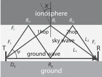
Fig. 1. VLF/LF propagation modeling (ground wave and sky waves).

2 Subionospheric VLF/LF propagation in terms of wave-hop method

The wave-hop method used in this paper is principally based on ray theory, but it takes into account the wave intensity as well as the wave ray-path computation. The wave-hop method is described briefly here. The wave received at a receiver is composed of ground wave and sky waves prop-agated in the Earth-ionosphere waveguide. The computation of sky waves is principally based on the ray theory, and the ground wave is calculated by the full-wave Sommerfeld inte-grations. More details are given in ITU (1992, 2002), Wakai et al. (2004) and its successful use has been given in Biagi et al. (2006). The configuration of our problem is given in Fig. 1, in which you can notice a 1-hop sky wave and a 2-hop sky wave. Generally, we can include many higher-2-hop waves, such as n-hop wave (n: the number of reflection from the ionosphere). In the case of 1-hop wave, the reflection point of the ionosphere is located just in the middle between the transmitter and receiver. The reflection coefficient at the ionosphere is defined by Ri. The ionospheric height is a function of the solar zenith angle (χ ), so that the launch-ing elevation angle (ψ) and path length (L) are determined by the distance between the transmitter and receiver (d) and ionospheric height (h). Though Fig. 1 is illustrated for a flat configuration, the real situation is for curved Earth and iono-sphere, and this results in an additional effect of focussing expressed by Fi (focussing at the ionosphere). With taking all effects into account, the electric field at the receiving point is given by, E1= 600 √ Ptcos ψ RiFiFtFr L1 (1) where Pt is the transmission power, Ft, Fr are transmitting and receiving antenna coefficients, respectively, which are

φ

φ

E

E

E

E

Fig. 2. Phasor diagram to have the resultant wave (as the

superposi-tion of ground wave and sky waves 1-hop and 2-hop waves). Etotal

is the total resultant wave, while Es1and Es2are the 1-hop and

2-hop waves, with φ₁and φ₂being their phase delay with respect to

the ground wave.

determined by the frequency and elevation angle (ψ). These antenna coefficients are just those converting the electric field into the voltage. L1is the total path length.

When we consider a 2-hop wave, the wave suffers from the ionospheric reflections twice and one ground reflection. The reflection coefficients for this case are given by Ri1, Ri2,

and Rg. In contrast to the focussing at the ionosphere, we expect the divergence at the ground, which is expressed by another coefficient, Dg. L2is the total path length for this

2-hop wave. The electric field at the receiver is given by the following equation for the 2-hop wave.

E2=600 √

Ptcos ψRi1Ri2Fi1Fi2RgDgFtFr

L2

(2) Generally speaking, the reflection and focussing coefficients of the ionosphere are not constant. On the assumption that the ionosphere is uniform over a relatively short distance, we assume that the ionosphere is uniform over a relatively short distance, and we assume that the ionospheric reflection coef-ficients are equal (Ri1=Ri2)and constant and also the

iono-spheric height (h) is also constant. Further, we can assume the relationship of Fi. ·Dg=1, and Eq. (2) is reduced to,

E2=

600√Ptcos ψR2iFiRgFtFr L2

(3) Generally the n-hop wave is also expressed by,

En=

600√Ptcos ψ RniFiRn−1g FtFr Ln

(4) We have to sum up the 1-hop, . . . . and n-hop waves to have a resultant field. In this paper we assume a relatively short

0 20 40 60 80 100 0 500 1000 1500 2000 Amplitude [ dB ] distance [ km ] hop1 hop1,2 hop1-3 ground wave 0 20 40 60 80 100 0 500 1000 1500 2000 Amplitude [ dB ] distance [ km ] hop1 hop1,2 hop1-3 ground wave 0 20 40 60 80 100 0 500 1000 1500 2000 Amplitude [ dB ] distance [ km ] hop1 hop1,2 hop1-3 ground wave

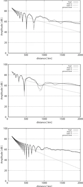
Fig. 3. Subionospheric electric field at the receiver as a function of propagation distance from the transmitter. (a) 40 kHz, (b) 20 kHz and (c) 100 kHz.

propagation distance of 1000–2000 km, so that it is found that we have to consider only up to a few-hop waves.

Figure 2 illustrates the phasor diagram, in which the total resultant wave (Etotal) is a sum of the ground wave (Eg) and

0 20 40 60 80 100 0 6 12 18 24 Amplitude [ dB ] L.T. Resultant wave ground wave sky wave 0 20 40 60 80 100 0 6 12 18 24 Amplitude [ dB ] L.T. Resultant wave ground wave sky wave

Fig. 4. (a) Diurnal variations of the electric field intensity for the ground wave (broken line), sky waves (dot-broken line) and resul-tant wave (full line) for the JJY-Kochi path. (b) Durnal variation of reflection height (full line) and phase delay of the 1-hop wave

with respect to the ground wave (φ₁). The bottom is the resultant

terminator time.

two sky waves (1-hop wave Es1and 2-hop wave Es2). Here, φ1and φ2are their phase delays relative to the ground wave

(Eg), which are resulted from the optical path difference and from the reflection at the iohosphere. However, when the propagation distance (d) is relatively small, the phase shift in the ionosphere is negligible, so that the phase delay of the sky wave with respect to the ground wave (L: total path length) is given by,

φ ∼₌ 2π

λ (L − d) (5)

3 Computational results on terminator times

Our Japanese VLF/LF network is consisted of seven receiv-ing stations (Moshiri (Hokkaido), Chofu, Chiba (Tateyama), Shimizu, Kasugai, Maizuru, and Kochi). We observe,

132 M. Yoshida et al.: On the generation mechanism of terminator times in subionospheric 0 20 40 60 80 100 0 6 12 18 24 Amplitude [ dB ] L.T. 20kHz 40kHz 100kHz

Fig. 5. Diurnal variation of the resultant electric field intensity for different frequencies (20, 40 and 100 kHz) for a fixed distance of 780 km. 0 20 40 60 80 100 0 6 12 18 24 Amplitude [ dB ] L.T. 800km 140km 2000km

Fig. 6. Diurnal variation of the resultant electric field intensity at f=40 kHz (JJY case) with changing the propagation distance (800, 140 and 2000 km).

at each station, simultaneously several VLF/LF transmit-ters; (i) NWC (Australia, f=19.8 kHz), (ii) NPM (Hawaii, 21.4 kHz), (iii) NLK (USA, 24.8 kHz), (iv) JJI (Kyushi, Ebino, f=22.2 kHz) and (v) Japanese standard wave trans-mission, JJY (f=40 kHz) (in Fukushima prefecture). This VLF/LF network is established for the study of seismo-ionospheric perturbations (Hayakawa et al., 2004). In the following we pay our main attention to the JJY transmitter, because this transmitter is located approximately in the mid-dle of Japan and the distance from this transmitter to each observing station is at close distances.

Figure 3a illustrates the distance dependence of the elec-tric field intensity in a test direction from JJY (geographic cooridinates: 37◦₂₂′_{N, 140}◦₅₁′_{E) to Kochi station (the} az-imuthal direction from JJY to Kochi station is 242◦_{from the}

0 20 40 60 80 100 0 6 12 18 24 Amplitude [ dB ] L.T. 40kHz hr+0 40kHz hr-3 40kHz hr+3 20kHz hr+0 20kHz hr-3 20kHz hr+3 0 20 40 60 80 100 0 6 12 18 24 Amplitude [ dB ] L.T. 0 20 40 60 80 100 0 6 12 18 24 Amplitude [ dB ] L.T. 100kHz hr+0 100kHz hr-3 100kHz hr+3

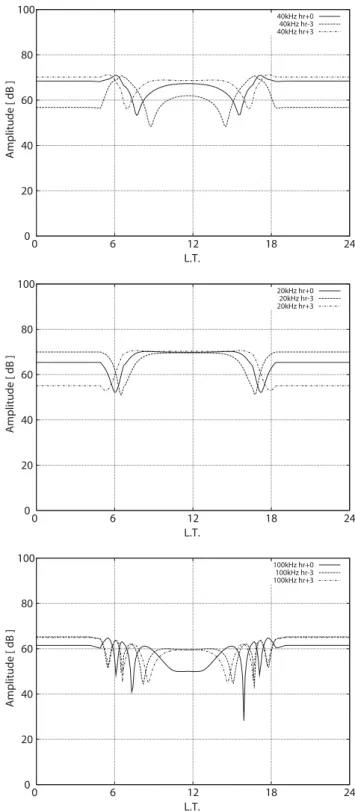
Fig. 7. Effects of shift in ionospheric reflection height on the diurnal amplitude variation. (a) 40 kHz, (b) 20 kHz and (c) 100 kHz.

North). The Earth’s magnetic field effect is also included in this computation. When we specify the location (lati-tude and longi(lati-tude) of the mid-point between the transmit-ter and receiver (in the case of 1-hop ray), relevant month

and local time, solar activity etc., we can determine the iono-spheric profile. So that we are ready to compute the matrix ionospheric reflection coefficients for our relevant frequency and incident direction (incident and azimuthal angles) at the relevant mid-point of reflection, with taking into accout the Earth’s magnetic field effect (Budden, 1961). The coefficient of reflection Ri in Eqs. (1), (3) and (4) is approximated by that ofqRq(TM incident, TM reflected) in the matrix iono-spheric reflection coefficients. The Rg is computed by the Fresnel coefficient. The frequency of JJY is 40 kHz, and its radiation power is 50 kW. The ionospheric height h is a function of solar zenith angle (Belrose, 1968) and it is about 75 km at day and 95 km at night. The coefficients Ri, Fi, and Dgare parameters depending on frequency and distance. For example, Fi∼_{=1.13, F}t∼_{=0.9, F}r∼_{=0.9 are used in the} compu-tations. Figures 3a–c are the figures of electric field inten-sity as a function of distance up to d=2000 km. The full line refers to 1-hop wave, the dotted lines, the results for up to 2 hops (i.e. 1-hop+2-hop), and the dot-full lines, those up to 3-hop wave. The ground wave is expressed by the broken line in these figures. Figure 3a refers to the JJY case (40 kHz), while Figs. 3b and 3c correspond to the lower transmission frequencies of 20 kHz and 100 kHz, but at the same place of transmission. It is found from a comparison of these figures that the effect of higher-hop sky waves increases with the in-crease in propagation distance. This is easily understood.

4 Generation mechanism of terminator times in subionospheric VLF/LF diurnal variation

We here consider a short-distance propagation condition, in which the transmitter is JJY station (frequency=40 kHz) and the receiver is located at Kochi (geographic coordi-nates; 33.55◦_{N, 133.53}◦_{E). So the propagation distance is} d=786 km. With taking into account the results in the pre-vious section, we have taken into consideration up to 2-hop waves. Figure 4a is the computed diurnal variation of the electric field intensity at the receiver. The broken line refers to the ground wave, the dot-broken line, to the sky waves, and the full line is the resultant wave. We notice clearly the presence of so-called terminator times with amplitude min-ima. We will show how these terminator times are formed. As is shown in Fig. 4a, the amplitudes of the ground and sky waves do not exhibit any significant diurnal changes. While, Fig. 4b illustrates the corresponding diurnal variations of re-flection height and phase delay of only 1-hop sky wave with respect to the ground wave (φ1in Fig. 2) (middle panel)

(be-cause the 2-hop wave is much weaker than the 1-hop wave, so that it is not considered here). It is found that when the phase delay φ1is 180◦, we have terminator times in the

di-urnal variation. So that, we can conclude that the terminator time is formed as an interference between the ground wave and sky wave.

-2.5 -2 -1.5 -1 -0.5 0 0.5 1 1.5 2 2.5 -6 -4 -2 0 2 4 6

terminator time shift [ hour ]

TTM TTE

variation of ionospheric reflection height [ km ]

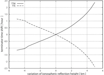
Fig. 8. The relationship between the terminator time shift and the change of ionospheric height. – means lowering, while + indicates upward shift of the lower ionosphere. Both terminator time evening (TTE) and terminator time morning (TTM).

For the fixed propagation distance from the JJY transmit-ter to Kochi (d=786 km), we have changed the frequency and Fig. 5 is the result on the terminator times. At lower frequen-cies of 20 and 40 kHz, we have one minimum around sunrise and sunset, while we have two terminator times around sun-rise and sunset for 100 kHz, simply due to a smaller wave-length of 100 kHz.

While, in Fig. 6 we have fixed the frequency of 40 kHz (JJY case) and for a fixed azimuth from the JJY to Kochi, but we have changed propagation distance (from 800 km to two values smaller and greater than 800 km i.e., 140 km and 2000 km). Figure 6 indicates that the terminator time appears very clearly for shorter distances of 800 km. When the dis-tance becomes smaller (140 km), we can espect some termi-nator time effect even though the ground wave is much more dominant than the sky wave. But, no terminator time appears for 2000 km.

5 Application of the terminator time to seismogenic study

As is already shown by Hayakawa et al. (1996) and Molchanov et al. (1998), the significant shift in termina-tor time for the Kobe earthquake over a short distance of

∼1000 km was interpreted in terms of a few km depletion of

the lower ionosphere before the earthquake by using the full-wave method. We assume the propagation path from JJY to Kochi. The frequency is widely varied from 40 kHz of our main interest to 20 and 100 kHz. The lower ionosphere is shifted in height by −3 km, −2 km, −1 km (these three, downward shifting), +1 km, +2 km and +3 km (upward shift-ing). Figure 7 illustrates the effect of shift in ionospheric reflection height on the diurnal variation. Figure 7a refers to

134 M. Yoshida et al.: On the generation mechanism of terminator times in subionospheric 40 kHz (JJY case), in which the full line refers to the case

of no perturbation and the broken line refers to the lowering the ionospheric and the dot-broken line corresponds to the upward shift of the ionosphere. When the ionosphere is low-ered, the morning terminator time shifts to early hours and the evening terminator time to later evening. That is, we can say that the daytime felt by the waves becomes longer. This is in excellent agreement with former experimental results (Hayakawa et al., 1996; Maekawa et al., 2006). The similar tendency can be confirmed for other frequencies in Figs. 7b and 7c.

Finally, we show the quantitative estimation on the rela-tionship between the shift in terminator time (terminator time morning TTM and terminator time evening TTE) and the change in ionospheric height. The transmitter and receiver are fixed to JJY (f=40 kHz) and Kochi, and Fig. 8 illustrates the corresponding results. When the ionosphere is lowered as in the case of earthquakes (Hayakawa et al., 1996), TTE shifts to later hours and TTM shifts to earlier hours. When

1_{h=−2 km, the shifts in both TTE and TTM are found to be}

of the order of 0.5 h (30 min), which are usually observed in the experiments. This figure will enable us to infer the in-formation on the perturbation of lower ionosphere before the earthquake. Hence, short (but not too short) distances (from a few hundred to 2000 km) offer a higher sensitivity for detect-ing the ionospheric modifications includdetect-ing those originatdetect-ing from seismic activity.

6 Conclusions

The generation mechanism of terminator times in subiono-spheric VLF/LF propagation has been studied for relatively short distances (less than 2000 km), and it is found that the terminator time is formed as an interference between the ground wave and sky wave. Finally, the relationship be-tween the terminator time shift and change in the ionospheric height, has been investigated, which suggests its possible use in inferring the lowering of the ionosphere before the earth-quakes.

Acknowledgements. The authors would like to thank NiCT for its

support (R and D promotion scheme funding international joint research).

Edited by: M. Contadakis

Reviewed by: P. F. Biagi and A. Nickolaenko

References

Belrose, J. S.: Low and very low frequency radio wave propaga-tion, in Radio Wave Propagapropaga-tion, AGARD Lecture Ser., 29, 97– 115, Advisory Group for Aerospace Research and Development, NATO, France, 1968.

Biagi, P. F., Castella, L., Maggipinto, T., Ermini, A., Perna, G., and Capozzi, V.: Electric field strength analysis of 216 and 270 kHz broadcast signals recorded during 9 years, Radio Sci., 41, RS4013, doi:10.1029/2005RS003296, 2006.

Budden, K. G.: The Wave-Guide Mode Theory of Wave Propaga-tion, Logos Press, London, 325 pp., 1961.

Hayakawa, M. and Molchanov, O. A.: Seismo Electromagnetics: Lithosphere – Atmosphere – Ionosphere Coupling, TERRAPUB, Tokyo, 477 pp., 2002.

Hayakawa, M. and Fujinawa, Y.: Electromagnetic Phenomena Re-lated to Earthquake Prediction, Terra Sci. Pub. Co., Tokyo, 667 pp., 1994.

Hayakawa, M., Molchanov, O. A., Ondoh, T., and Kawai, E.: The precursory signature effect of the Kobe earthquake on VLF subionospheric signals, J. Comm. Res. Lab., Tokyo, 43, 169– 180, 1996.

Hayakawa, M.: Atmospheric and Ionospheric Electromagnetic Phenomena Associated with Earthquakes, Terra Sci. Pub. Co., Tokyo, 996 pp., 1999.

Hayakawa, M. and Molchanov, O. A.: NASDA/UEC team, Sum-mary report of NASDA’s earthquake remote sensing frontier project, Phys. Chem. Earth, 29, 617–625, 2004.

International Telecommunication Union, Recommendation ITU-R, Ground wave propagation curves for frequencies between 10 kHz and 3 DMHz,Geneva, Switzerland, P. Series, p. 368–7,1992. International Telecommunication Union, Recommendation

ITU-R, Prediction of field strength at frequencies below 150 kHz, Geneva, Switzerland, P. Series, p. 684-3, 2002.

Maekawa, S., Horie, T., Yamauchi, T., Sawaya, T., Ishikawa, M., Hayakawa, M., and Sasaki, H.: A statistical study on the effect of earthquakes on the ionosphere, based on the subionospheric LF propagation data in Japan, Ann. Geophys., 24, 2219–2225, 2006,

http://www.ann-geophys.net/24/2219/2006/.

Molchanov, O. A. and Hayakawa, M.: Subionospheric VLF signal perturbations possibly related to earthquakes, J. Geophys. Res., 103, 17 489–17 504, 1998.

Molchanov, O. A., Hayakawa, M., Ondoh, T., and Kawai, E.: Pre-cursory effects in the subionospheric VLF signals for the Kobe earthquake, Phys. Earth Planet. In., 105, 239–248, 1998. Rozhnoi, A., Solovieva, M. S., Molchanov, O. A., and Hayakawa,

M.: Middle latitude LF (40 kHz) phase variations associated with earthquakes for quiet and disturbed geomagnetic conditions, Phys. Chem. Earth, 29, 589–598, 2004.

Shvets, A. V., Hayakawa, M., Molchanov, O. A., and Ando, Y.: A study of ionospheric response to regional seismic activity by VLF radio sounding, Phys. Chem. Earth, 29, 627–637, 2004. Wakai, N., Kurihara, N., Otsuka, A., and Imamura, K.:

Predic-tion method of LF/MF field strangths, Inst. Electr. InformaPredic-tion Comm. Engrs. Japan, Technical Report, AP-2003-271, 35–40, 2004.