HAL Id: hal-00304649
https://hal.archives-ouvertes.fr/hal-00304649
Submitted on 1 Jan 2002HAL is a multi-disciplinary open access archive for the deposit and dissemination of sci-entific research documents, whether they are pub-lished or not. The documents may come from teaching and research institutions in France or abroad, or from public or private research centers.
L’archive ouverte pluridisciplinaire HAL, est destinée au dépôt et à la diffusion de documents scientifiques de niveau recherche, publiés ou non, émanant des établissements d’enseignement et de recherche français ou étrangers, des laboratoires publics ou privés.
a Genetic Algorithm approach
A. V. M. Ines, P. Droogers
To cite this version:
A. V. M. Ines, P. Droogers. Inverse modelling in estimating soil hydraulic functions: a Genetic Algorithm approach. Hydrology and Earth System Sciences Discussions, European Geosciences Union, 2002, 6 (1), pp.49-66. �hal-00304649�
Inverse modelling in estimating soil hydraulic functions: a Genetic
Algorithm approach
Amor V.M. Ines
1and Peter Droogers
1,a1 International Water Management Institute P.O. Box 2075 Colombo, Sri Lanka
1,a Water Engineering and Management Program, School of Civil Engineering,Asian Institute of Technology P.O. Box 4 Klong Luang 12120 Pathumthani, Thailand
Email for corresponding author: [email protected]
Abstract
The practical application of simulation models in the field is sometimes hindered by the difficulty of deriving the soil hydraulic properties of the study area. The procedure so-called inverse modelling has been investigated in many studies to address the problem where most of the studies were limited to hypothetical soil profile and soil core samples in the laboratory. Often, the numerical approach called forward-backward simulation is employed to generate synthetic data then added with random errors to mimic the real-world condition. Inverse modelling is used to backtrack the expected values of the parameters. This study explored the potential of a Genetic Algorithm (GA) to estimate inversely the soil hydraulic functions in the unsaturated zone. Lysimeter data from a wheat experiment in India were used in the analysis. Two cases were considered: (1) a numerical case where the forward-backward approach was employed and (2) the experimental case where the real data from the lysimeter experiment were used. Concurrently, the use of soil water, evapotranspiration (ET) and the combination of both were investigated as criteria in the inverse modelling. Results showed that using soil water as a criterion provides more accurate parameter estimates than using ET. However, from a practical point of view, ET is more attractive as it can be obtained with reasonable accuracy on a regional scale from remote sensing observations. The experimental study proved that the forward-backward approach does not take into account the effects of model errors. The formulation of the problem is found to be critical for a successful parameter estimation. The sensitivity of parameters to the objective function and their zone of influence in the soil column are major determinants in the solution. Generally, their effects sometimes lead to non-uniqueness in the solution but to some extent are partly handled by GA. Overall, it was concluded that the GA approach is promising to the inverse problem in the unsaturated zone.
Keywords: Genetic Algorithm, inverse modelling, Mualem-Van Genuchten parameters, unsaturated zone, evapotranspiration, soil water
Introduction
In developing improved water management alternatives, physically-based simulation models could be helpful. These simulation models can be used as tools to understand the current system better since they provide information over an unrestricted spatial and temporal resolution. Models are also strong in providing information about processes that are difficult to measure in the field such as capillary rise, soil evaporation and crop transpiration. Most important is their ability to do scenario analysis as they can integrate easily the impacts of any changes to the system. However, an obstacle to their practical application in the field is the difficulty of deriving the soil hydraulic functions θ(h) and
K(h) of the study sites, where θ is the soil water, h is the hydraulic head and K is the unsaturated hydraulic conductivity. This seems to be of minor concern in conventional thinking but inevitably the veracity of the input data will be reflected in the end. According to Xevi et al. (1996) proper evaluation of the water balance in the unsaturated zone depends strongly on the appropriate characterisation of the soil hydraulic functions. Therefore, proper definition of the soil hydraulic parameters under field conditions should be taken into consideration.
Direct measurement in the laboratory using soil core samples is the classic way to determine the soil hydraulic functions (Van Genuchten et al., 1991). Although this is
relatively easy in principle, in practice it is difficult and time-consuming. To obtain sets of soil water at different hydraulic heads also needs specialised apparatus; likewise for conductivity values. The major concern with this approach is the question of whether the parameters derived in a soil core sample with pre-defined boundary conditions are representative of the field situation (Kool and Parker, 1988; Van Dam, 2000). A broad range of field methods was also developed to determine the soil hydraulic functions (Dirksen, 1991).
Using pedo-transfer functions is another approach, where soil texture, bulk density and organic matter content are used to estimate soil hydraulic parameters (e.g. Vereecken et al., 1989, 1990; Wösten et al., 1998; Droogers et al., 2000; Antonopolous, 2000). These are very useful functions if limited information is available about the soil. However, Wösten et al. (1998) stressed the need for further research to develop a more robust and efficient methodology that could estimate soil hydraulic parameters practically for real-world applications.
The potential of a heuristic approach to estimate the Mualem-Van Genuchten parameters has been investigated recently. Schaap et al. (1998) studied 19 Hierarchical Neural Network (HNN) models (based on the input data) and found that the accuracy of the prediction improved when more input data were used. They concluded that the developed HNN models performed better than the published pedo-transfer functions in predicting soil water and hydraulic conductivity parameters. The use of the HNN models developed is claimed to be attractive because of the considerable flexibility toward available input data.
The inverse modelling approach is also applied where the measured soil hydraulic data are used as fitting criteria to estimate the soil hydraulic parameters by inverting the governing equation of the soil water movement. The inverse approach has been implemented extensively in groundwater studies (e.g. Yeh, 1986). The obvious reason is that direct measurement of aquifer characteristics is far more difficult than in the vadoze zone. Using observed pressure heads and measured discharges, the transmissivity, specific yield, storage coefficient and other aquifer parameters could be determined by the inverse solution of the groundwater flow equation. Yeh (1986) reviewed the common techniques to solve the inverse problem in the saturated zone. The review showed that the problem could be solved using either a direct (equation error criterion) or an indirect approach (output error criterion). The indirect approach is more attractive because it does not require spatial and temporal data at regular intervals, hence avoiding the interpolation of data from sparse observations which could increase the noise in the dataset. Gradient-dependent search algorithms are
widely used in this case. Non-linear regression is also adopted, e.g. MODFLOWP (Hill, 1992), the ModGA_P used a Genetic Algorithm (Zheng, 1997).
Kool and Parker (1988) solved the inverse problem in unsaturated transient flows using the indirect approach with the Levenberg-Marquardt algorithm. The Richards’ equation was solved inversely during infiltration and redistribution in a hypothetical soil profile to determine the soil hydraulic functions simultaneously. The soil water and hydraulic head were used as fitting criteria. Based on their works (Kool et
al., 1985; Kool and Parker, 1988), several studies were
conducted to investigate the inverse problem in unsaturated flows further. The method has been applied with reasonable success in the laboratory using outflow experiments such as the one-step (e.g. Van Dam et al., 1992) and multi-step outflow approach (e.g. Van Dam et al. 1994; Zurmühl and Durner, 1998) where the measured outflow and soil water (in some cases) were used as fitting criteria in estimating the soil hydraulic parameters. In contrast, Šimùnek et al. (1998) and Romano and Santini (1999) among others approached the inverse problem using the evaporation method (which is the opposite of the outflow experiments) where the soil water and hydraulic heads were usually used as criteria. In general, most of the literature about the inverse approach always emphasised the ill-posed nature of the solution. This is caused mainly by (1) the non-uniqueness problem and (2) instability in the solution. The non-uniqueness problem occurs when the parameters under study have low sensitivity to the criteria being investigated. This could happen in the solution because at some point in the search space, the parameter(s) may not be sensitive any longer. This problem is also caused by local optima and is a threat to gradient-dependent search algorithms. The instability problem, on the other hand, is caused by the high sensitivity of the parameters (Yeh, 1986; Kool and Parker, 1988; Van Dam et al., 1992).
The inverse modelling approach seems to be a very promising way to estimate soil hydraulic functions in the unsaturated zone where most plant activities are concentrated. However, the fitting criteria used in previous studies are mostly the soil water, hydraulic head and bottom flux. Soil water can be monitored easily in the field but bottom fluxes are more difficult to measure. Hydraulic heads can be measured using tensiometers. It seems that broader application of the methodology in the field depends strongly on the practicality of the criteria being used in terms of spatial and temporal dimensions. Evapotranspiration could be explored in this case because: (1) it can be estimated or measured easily (Kite and Droogers, 2000) and (2) it has an advantage in larger scale applications (e.g. an irrigation system) using remote sensing data e.g. SEBAL
(Bastiaanssen et al., 1998). In a recent study (Jhorar et al., 2002), the use of evapotranspiration as a criterion was investigated in inverse modelling using SWAP (Van Dam
et al., 1997) and a parameter estimation package, PEST
(Watermark Computing, 1994). The actual evapotranspiration and actual transpiration were used as criteria, separately. The benchmark values of the criteria were established using forward simulation by assuming some base values of the Mualem-Van Genuchten parameters and then backward simulations were done to obtain the parameters again. To emulate the real-world situation, random errors were included in the benchmark values. In reality, actual transpiration is difficult to obtain separately from evapotranspiration. Therefore, evapotranspiration alone is more realistic to explore as a criterion in inverse modelling. On this basis, robust search algorithms are needed to investigate this option further. A heuristic yet powerful search technique like Genetic Algorithms could be suitable in this case.
In summary, the objectives of this paper are: (1) to explore the inverse problem in the unsaturated zone using evapotranspiration, soil water and the combination of both, as fitting criteria, numerically, (2) the same, but using measured evapotranspiration and soil water from lysimeter data, and (3) to investigate the potential of Genetic Algorithms in the solution of the inverse problem and how the technique handles the issues of non-uniqueness and instability.
Methodology
SIMULATION MODELThe Soil Water Atmosphere and Plant model generally known as SWAP (Van Dam et al., 1997) is a physically based, detailed agro-hydrological model that simulates the relationships of the soil, water, weather and plants. The core of the model is the Richards’ equation (Eqn. 1) where the transport of soil water is modelled by combining Darcy’s law and the law of continuity:
( )
( )
S( )
h z z h h K t h h C t ∂ − + ∂ ∂ ∂ = ∂ ∂ = ∂ ∂θ 1 (1)where θ is the soil water content (cm3 cm-3), h the hydraulic
head (cm), C the water capacity (cm-1), t the time (d), z the
vertical distance taken positive upward (cm), K the unsaturated hydraulic conductivity (cm d-1) and S is the sink
term (d-1). SWAP models the soil water movement by
considering the spatial and temporal differences of the soil water potentials in the soil profile. The governing equation
is solved numerically with the implicit scheme of Belmans
et al. (1983), which can be applied effectively in saturated
and unsaturated conditions.
In SWAP, the soil hydraulic functions are described by the analytical functions of Van Genuchten (1980) and Mualem (1976) for the soil water retention (Eqn. 2) and hydraulic conductivity (Eqn. 3) referred hereafter as MVG:
( )
[
n]
m res sat res h h α θ θ θ θ + − + = 1 (2)( )
2 1 1 1 − − = m m e e satS S K h K λ (3) where θres is the residual soil water content (cm3 cm-3), θsatthe saturated soil water content (cm3 cm-3), α (cm-1), n (–),
m (–) and λ (–) are empirical shape parameters and Ksat is
the saturated hydraulic conductivity (cm d-1). Equations 4a
and 4b define the relative saturation, Se (–) and parameter m (–):
( )
res sat res e h S θ θ θ θ − − = (4a) n m=1−1 (4b)SWAP does not only simulate the quantity of soil water but also the quality and considers the effect of heat on the fate of solutes. Hysteresis, water repellency, soil swelling and shrinkage can be also assumed to affect soil water and solute transport. For this study these options were not employed. The water balance is solved by considering two boundary conditions, the top and bottom boundaries. These boundaries can be either flux or head controlled. The Penman-Monteith equation is used to estimate evapotranspiration. SWAP uses the leaf area index (LAI) or soil cover fraction (SC) to calculate the potential transpiration and evaporation of a partly covered soil. The model separates firstly the potential transpiration (Tp) and potential evaporation (Ep) then subsequently calculates the reduction of Tp in a more physically based approach (Feddes et al., 1978; Maas and Hoffman, 1977). The compounded effect of salt and water/ oxygen stress to the actual transpiration (Ta) is considered multiplicative. In the case of wet soil, the soil evaporation is determined by the atmospheric demand and is equal to
Ep.However, as the soil dries, the soil hydraulic conductivity also decreases and the evaporation is decreased to actual evaporation (Ea). The maximum evaporation (Emax) is calculated using Darcy’s law at the top boundary, then Ea is
computed as the minimum of Ep and Emax. Alternatively, the soil evaporation can be estimated using the empirical equations of Black et al. (1969) or Boesten and Stroosnijder (1986). In general, the actual evaporation is calculated as the minimum of Ep, Emax and the Ea using the empirical functions.
The surface runoff is calculated as the ratio of the difference between the depth of ponding water and the maximum sill (embankment) height to the resistance of the soil to surface runoff. The surface detention is accounted for in the resistance term. Field drainage can be simulated using the Hooghoudt and Ernst equations in homogenous and heterogeneous soil profiles. Drainage systems can be modelled as a single or multi-level system. Bottom flux is calculated according to the bottom boundary condition adopted in the model.
A simple crop model and detailed crop model WOFOST can simulate crop growth in SWAP. The simple crop model is based on the linear production function of Doorenbos and Kassam (1979). WOFOST (Supit et al., 1994) is a generic crop model, capable of simulating the growth and development of most crops. In this study, the detailed crop model was used.
Several water management scenarios can be modelled in SWAP. Irrigation scheduling can be considered as fixed time or according to a number of criteria. A combination of irrigation prescription and scheduling is also possible. The scheduling criteria define the timing and depth of irrigation in the growth process.
GENETIC ALGORITHMS
Genetic Algorithms (GAs) are mathematical models of natural genetics where the power of nature to develop, destroy, improve and annihilate life is abstracted and used to solve complex optimisation problems. Holland (1975) developed this powerful technique and it has been applied in various fields of science. GA is termed a global optimum-seeking algorithm (Zheng, 1997). The algorithm works by mimicking the mechanisms of natural selection to explore decision search space for optimal solutions (Goldberg, 1989).
Goldberg (1989) identified four unique attributes of GA (binary) among the more traditional optimization methods: (1) GA works with a coding of the parameter set (string), not with the parameters themselves, (2) GA searches from a population of points, not a single point, (3) GA uses objective function information, not derivatives or other auxiliary knowledge and (4) GA uses probabilistic transition rules, not deterministic rules.
GA consists of three basic operators: the selection,
crossover and mutation (Cieniawski et al., 1995). First, an initial set of individuals (strings) is generated. This population is a representative set of solutions to the problem under investigation. Each individual is evaluated on its performance with respect to some fitness function which represents the environment. Using this measure, the individual competes in a selection process where the fittest survives and is selected to enter the mating pool; the lesser-fit individual dies. The selected individuals (parents) are assigned a mate randomly. Genetic information is exchanged between the two parents by crossover to form offspring. The parents are then killed and replaced in the population by the offspring to keep the population size stable. Reproduction between the individuals takes place with a probability of crossover. If a random number generated is less than the probability of crossover, crossover happens, otherwise not, and the parents enter into the new population. GAs are very aggressive search techniques; they tend to converge quickly to a local optimum if the only genetic operators used are selection and crossover. The reason is that GA eliminates rapidly those individuals with poor measures until all the individuals in the population are identical. Without a fresh influx of new genetic materials, the solution stops there. To maintain diversity, some of the genes are subjected to mutation to keep the population from premature convergence (Goldberg, 1989; Cieniawski et al., 1995). Selection, crossover and mutation are repeated for many generations, with the expectation of producing the best individual(s) that could represent the optimal or near optimal solution to the problem under study.
In this study, a modified-µGA was developed and used in the inverse modelling. This is a slight modification of the securGA (small-elitist-creep-uniform-restarting GA) of Carroll (in Yang et al., 1998). The µGA technique (Krishnakumar, 1989; Caroll, 1996, 1998) was extended to enable creep mutation to take place in the solution (securGA). In complex problems, however, more individuals might be needed to arrive at the best solution. In the securGA, the innate nature of convergence of a µGA is still being used, i.e. 95% uniformity of the genes which suppressed the restarting power of a µGA in larger populations. For this reason, a 90% convergence is used in the modified-µGA.
SWAP-GA LINKAGE
Figure 1 shows the linkage between SWAP and GA. The fitness function serves as an environment for the thriving population in each generation. The fitter individuals (represented by a high value of fitness) that survived the test of the environment tend to reproduce and produce
offspring that are expected to express better genetic traits in the next generation, to cope up with the environmental demands. In this study, the fitness function used is expressed as follows:
(5)
where ξ is a weighting factor (–), θSWAP and θOBS are the soil
water content simulated and observed, respectively (cm3 cm-3), ET
aSWAP and ETaOBS the actual evapotranspiration
simulated and observed, respectively (cm d-1), T is an index
of year, i is for day, j is for soil compartment, k represents an individual in the GA, N and M are indices of the number of observations of θ and ETa and fitness is the measure of
an individual.
The θ and ETa are the criteria in the parameter estimation
and their contributions to the fitness function is determined by the weighting factor ξ. The observed and simulated soil water and ET values used in evaluating the fitness function are normalized using the observed minimum and maximum values of θ and ETa.
The Mualem-Van Genuchten (MVG) parameters in the SWAP-GA linkage are represented as binaries (0s and 1s), similar to the standard GA approach of multi-parameter representation (see Fig. 2), where P stands for parameter. The real value of a parameter is defined as:
(6)
where Cmax is the maximum value of the parameter and Cmin the minimum value, a represents alleles or bit value (0 or 1), i is an index of bit position (referred as gene), L is length of the (sub) string, and j, the index for parameter.
LYSIMETER
Lysimeter data (Tyagi et al., 2000) from a wheat (Triticum
aestivum) experiment in India (Karnal, Haryana) during the
1991–1992 rabi season were used in the study. The lysimeter is a weighing type, with a surface area of 4 m2 and depth of
2 m. Daily changes in lysimeter weight were recorded in a data logger and retrieved regularly. These weight changes were subsequently converted to equivalent actual ET. Accurate daily ET data could be generated from this experiment except when there is excessive rainfall or irrigation application. Weather data were monitored using a manual and an automatic weather station adjacent to the lysimeter site. In addition, data on crop, soil and water management practices were collected and recorded during the duration of the experiment. Percolation losses were collected from the sump located at the bottom of the lysimeter.
In the model set up, the soil profile was divided into two layers: 0-60 cm (31% sand, 50% silt, 19% clay) and 60–200 cm (29% sand, 49% silt, 22% clay). Soil water monitoring was done mostly in the first layer at four depths (0–15, 15–30, 30–45 and 45–60 cm) using a Time Domain Reflectometer (TDR). Soil water measurements were taken frequently at irregular intervals and a total of 31 observations were available. In the simulations, the soil column was assumed to be well drained.
Using the data on soil texture, bulk density and organic matter content, the estimates of the MVG parameters were derived with pedo-transfer functions (PTF) (Wösten et al., 1998; Droogers, 1999). These estimates (see Table 1) were used in the numerical study as parameter base values where the performance of GA to handle the non-uniqueness and instability issues was tested.
SENSITIVITY ANALYSES
The sensitivity of a parameter to the fitness function determines the success of the estimation of the parameter involved. A straightforward method was applied by first setting the MVG parameters at an initial value as close as + − =
∑∑∑
T i j SWAP OBSTij N k fitness 1 1 ) ( θ θ ξ(
)
− − +∑∑
T i ETaSWAP ETaOBSTi M 1 1 1 ξ ( ) ( )[
C ( )j C ( )j]
a j C j C j j L L i i i min max 1 1 1 min 2 2 − + = = − −∑
Table 1
. Summary of results in inverse modeling using a Genetic Algorithm.
A
verage Error
b
R
2, %
Predicted parameter values
Criteria Fitness θ ET a θ ET a Soil layer 1 (0-60 cm) Soil layer 2 (60-200 cm) Numerical case α nK sat θsat c α nK sat θsat Base values a 0.02100 1.2080 15.28 0.384 0.01800 1.1370 10.19 0.365
Daily data 4 parameters
ET a 1435.9 6.9E-3 3.9E-4 99.22 99.99 0.02010 1.2168 -0.02753 1.1678 -θ 14586.0 1.1E-5 1.7E-5 99.99 99.99 0.02099 1.2081 -0.01801 1.1370 -θ+ET a 2665.9 3.0E-3 1.1E-4 99.93 99.99 0.02023 1.2069 -0.02049 1.1468 -8 parameters ET a 3375.9 1.3E-1 1.7E-4 97.93 99.99 0.01678 1.1479 22.28 0.587 0.02318 1.1517 10.63 0.355 θ 284.1 5.5E-4 8.6E-4 99.97 99.99 0.02779 1.1881 28.09 0.391 0.03289 1.1080 34.55 0.372 θ+ET a 1522.1 5.3E-2 1.9E-4 99.30 99.99 0.02587 1.1580 36.87 0.449 0.04509 1.1 173 39.33 0.340 W eekly Data 4 parameters ET a 1500.6 1.3E-2 3.1E-4 99.34 99.99 0.01669 1.1957 -0.02721 1.1676 -θ 301.6 4.6E-4 3.4E-4 99.95 99.99 0.02125 1.2033 -0.01679 1.1372 -θ+ET a 1980.2 2.3E-2 1.2E-4 95.88 99.99 0.01668 1.1920 -0.03695 1.2145 -8 parameters ET a 6252.4 1.9E-2 7.4E-5 99.19 99.99 0.03396 1.1609 52.45 0.364 0.03517 1.0921 45.55 0.347 θ 61.2 2.3E-3 3.4E-3 97.20 99.98 0.02462 1.1987 21.04 0.392 0.04172 1.1496 35.14 0.403 θ+ET a 783.8 8.1E-2 2.9E-4 91.78 99.99 0.01666 1.1451 29.68 0.430 0.05683 1.1709 26.75 0.529
Experimental case Lysimeter data 4 parameters
ET a 8.4 1.7E-1 7.4E-2 54.67 77.73 0.04521 1.6285 -0.05778 1.2533 -θ 8.2 2.6E-2 7.5E-2 66.13 77.15 0.00782 1.7956 -0.01283 1.0813 -θ+ET a 8.3 2.6E-2 7.5E-2 67.20 77.18 0.00758 1.7976 -0.01089 1.0813 -8 parameters ET a 8.5 7.0E-2 7.4E-2 0.41 77.93 0.01703 2.1562 1.25 0.575 0.04317 1.1707 0.87 0.461 θ 8.7 2.4E-2 7.7E-2 62.37 77.79 0.00585 2.1493 54.42 0.407 0.01983 1.081 1 4.13 0.323 θ+ET a 8.1 2.8E-2 7.4E-2 57.02 77.52 0.01316 1.7818 2.55 0.568 0.04330 1.4522 4.66 0.587
a from pedo-transfer function (Wösten
et al
., 1998; Droogers, 1999);
θres
= 0.000 for both layers;
λ
= 2.523 and –3.997 for layer 1 and 2 respectively
. bθ(cm 3 cm -3); ET a (cm d -1)
c in the experimental case, predefined
θsat
possible to the expected value and then running the SWAP model. Subsequently, MVG parameters are changed from their initial values by a certain percentage and model output is compared to the output from the initial runs. A parameter change resulting in an insignificant change in output of the model indicates that the parameter considered is less important in the analysis. Moreover, such a parameter is very unlikely to be estimated successfully, as it is not affecting the fitness function used in the inverse modelling. The initial values of the parameters were set to the values obtained from the PTF as described above.
All six MVG parameters were subjected to this sensitivity analysis. Actual ET was selected as a criterion because it is included in the fitness function and ET can be considered as an integrated output from the complex soil-water-plant-atmosphere processes. A second criterion used was the flux at the bottom of the soil profile. The bottom flux also reflects the soil-water-plant interactions and can be considered as an integrated representation of the soil water status in the entire profile, which is the other component of the fitness function. Only the MVG parameters at the first soil layer were set as variables during the sensitivity analysis.
PARAMETER ESTIMATION CASES
Two main cases were considered to estimate the MVG parameters: (1) whether generated observations were used (the numerical case) and (2) whether real-life observations from the lysimeter experiment were used (the experimental case).
To evaluate the performance of GA, model-generated output was used first instead of actual field measurements, i.e. the numerical case. Such an approach is common in many studies, often extended with the incorporation of random errors in the generated “observations”. The MVG parameters as estimated from the PTF were considered for the numerical case as the real parameter values. The SWAP model was run with these parameters and the generated output was assumed in the inverse modelling as the “measured” values. The results from the sensitivity analyses, as presented later, were used to determine which parameters have to be estimated. However, it is well known that the inclusion of too many parameters in inverse modelling tends to result in non-uniqueness; therefore, the number of parameters for the first test was limited to two per soil layer (4-parameter problem) and in the second stage, four parameters per soil layer were considered (8-parameter problem).
In addition to these 4- and 8-parameter problems, two other cases were considered. First, the daily model output was used as the “measured” values and second, the daily model outputs were aggregated into weekly values. The
latter can be seen as a first step towards the experimental case where daily measurements are usually scarce, especially for soil water data.
The fitness function was constructed in such a way that different weights could be given to ET and soil water. For this study three options were considered: (1) only ET (ETa) was used in the fitness function (ξ = 0), (2) only soil water (θ) was used (ξ = 1) and (3) equal weights to soil water and ET (ξ = 0.5), a multi-objective situation (θ + ETa). Obviously,
additional values between 0 and 1 could be used but were not considered in this study.
For the experimental case, actual ET data as well as measured soil water contents were used in the fitness function. As in the numerical case, two different sets of parameters were estimated per soil layer: (1) α and n and (2) α, n, Ksat and θsat. Obviously, the situation is different
from the numerical case as the exact parameter values are unknown for the lysimeter experiment.
To summarize, 18 different cases were considered, based on the combinations of generated or measured data, two or four MVG parameters per soil layer, daily or weekly data and weights on ET and soil water (see Table 1).
Results and conclusions
SENSITIVITY ANALYSESA summary of the output generated by SWAP using the parameter values derived from PTF is presented in Fig. 3. The amounts of rainfall and irrigation were derived from the recorded daily changes of lysimeter weight. These were compared to the measured rainfall and irrigation during the experiment; the lysimeter was able to produce highly comparable values. The high sensitivity of the lysimeter allows the accurate measurements of the crop ET and thus increases the level of confidence in the analysis.
SWAP is able to partition the actual soil evaporation and plant transpiration. In the figure, the interception by the canopy during a rainfall event is incorporated in the evaporation. The crops were well watered during the experiment, no significant water stress is evident along the crop growth; only the minimal water stress experienced by the crops before the third irrigation (day 22) is apparent. The abrupt reduction in relative transpiration is mainly due to oxygen stress when the soil is saturated during an irrigation or rainfall. At some stages the crop could not recover immediately from oxygen deficiency, which can be noticed after the fourth irrigation followed by the succeeding rainfall events. This increase in water input is evident in the subsequently increased bottom flux during and after these periods. In the figure, the high quantity of bottom flux at
Fig. 3. Daily output of the SWAP model for the base case using pedo-transfer functions
the onset of simulation is due mainly to the initial condition used in the soil profile. All soil compartments were initialized at field capacity (h = –100 cm).
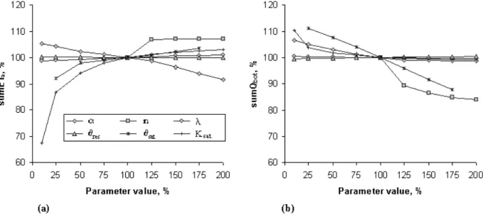
Before the start of the inverse modelling, the sensitivity of parameters was assessed to define the most applicable parameters to be optimised. The situation in Fig. 3 was used as a base scenario where the sum of the daily actual ET (sumETa) and bottom flux (sumQbot) were used as sensitivity
criteria. The results of the sensitivity analysis (Fig. 4a and b) indicate clearly that θres and λ are non-sensitive parameters
and can be ignored in further analyses: a change in one of these parameters does not affect the model output substantially. The other four parameters are sensitive in changing the model output; therefore, these could be included in the inverse modelling. Parameter n could be tested only for values higher than the original 100% as n
has a lower limit of 1 in the MVG equations. The sensitivity of Ksat was clearly limited to lower values, indicating that the parameter estimation by inverse modelling will yield reliable results only when the predicted Ksat values along the search are lower than the expected value. Interestingly, the θsat mainly affects the bottom flux while ET is only partly
affected. The results of the sensitivity analyses were used to select the number of parameters to be estimated as explained before, as shown in Table 1.
GENETIC ALGORITHM
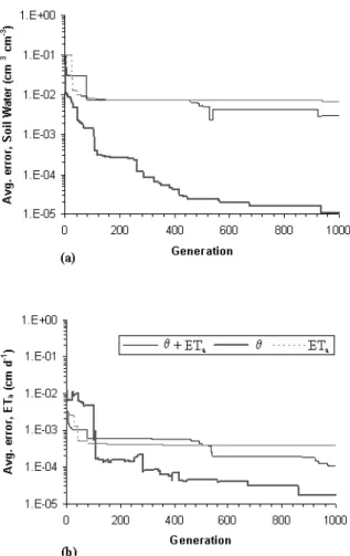
An example of a typical parameter estimation using GA is shown in Fig. 5a and b. The figures present the GA solutions of the 4-parameter problem using daily data in the numerical case with the three criteria being used (ETa, θ and θ + ETa).
The maximum and the average fitness show the typical behaviour of GA in comparison to other parameter estimation techniques. A maximum fitness value in a generation corresponds to the measure of the best individual in that instantaneous population for any of the fitting criterion mentioned above. The average value corresponds to the average fitness of the population. Fig. 5a shows that an elitist GA is not gradually moving to an optimum, but a stepwise improvement can be observed. After finding a new maximum fitness value, the corresponding parameter combination (individual) is tagged as elite and carries this identity along the generations until a new elite is found in the search. The GA continues the process of selection, crossover and mutation (creep) to search for new parameter combination that gives the best possible value of the fitness function until the end of the generations. In the numerical
Fig. 4 (a) Sensitivity analysis of the soil hydraulic parameters to ET. (b) Sensitivity analysis of the soil hydraulic parameters to bottom flux.
Fig. 5. (a) Maximum fitness values in a generation with the
modified-µGA solution (daily, 4-parameter). ETa indicates ET alone
as criterion, θ, soil water alone and θ + ETa, the combination.
(b) Average fitness values in a generation with the modified-µGA
case, the maximum number of generations was limited to 1000 while in the experimental case it was 2000. The longer timeline in the experimental case was intended to produce the best possible solution with the real-world condition. Further, the average fitness (Fig. 5b) shows how the GA exploited the micro population to explore the search space under each fitting criterion. When the average fitness is high and nearly touching the maximum fitness line, the population is composed of highly measured individuals and is near convergence. On the other hand, when the value is low, some or even the majority of the population are lowly measured individuals (as compared to the elite). This contrast, however, is necessary in the search because diversity means more genetic traits to be introduced in the generations, which is induced by the mutation and population restart mechanism. The crossover operation will exchange these genetic traits with the selected individuals.
The scope of the study is limited to the use of GA in the inverse problem. As such, the computational efficiency and accuracy of results were not compared with other methods. The computational efficiency, however, can be gauged by the GA parameters used in the search such as the number of individuals in a population and maximum number of generations. With the present computing capabilities, doing the GA processes (selection, crossover and mutation) alone is not as computationally intensive as compared with the time the integrated model SWAP takes to do the simulations for the evaluation of individual fitness. As observed, when the parameter combination is extreme, the model takes a long time to finish the simulation. As regards accuracy, the results to be discussed show that, in theory, GA is able to match the solution with high accuracy. In the study, the 4-and 8-parameter problems had a population size of 20 4-and 30, respectively. A 0.5 probability of crossover was used in all cases and the probability of creep mutation was taken as the reciprocal of the population size. In all cases, a random number seed of –1000 was used in the search.
NUMERICAL CASE
The results of the 12 cases considered in testing the performance of GA for the generated “observations” are given in Table 1. Considering the ability to match the “measured” and simulated values, the GA performance was thought to be excellent, with R2 in all cases higher than 91%
and in most cases even higher than 99%. The average error in ET was always lower than 0.003 cm d-1. However, average
deviations in soil water contents for the whole soil profile varied between 0.13 and almost 0 cm3 cm-3. In this study,
the soil profile is discretised into 33 compartments, i.e. 20 and 13 compartments for the first and second soil layers, respectively.
Figure 6a and b shows the reduction in the average errors between the “observed” and simulated ET and soil water contents during the GA search for the 4-parameter problem using daily data. In the case where only the soil water (θ) was included in the fitness function, the average error between the “observed” and simulated soil water contents was reduced rapidly during the first 400 generations. Interestingly, simultaneous reduction of the average error in ET was also substantial, particularly during the first 100 generations, then eventually decreasing with the soil water along the remaining generations. For the cases where only ET or soil water and ET (θ +ETa) were included in the fitness
function, the reduction in the average errors in soil water and ET are still very satisfactory: 0.007 and 0.003 cm3
cm-3, and 0.004 and 0.001 mm d-1, respectively. It is
interesting that optimising the fitness function using the soil water contents only also improved the ET solution.
Fig. 6.(a) Average error of soil water (q) in a generation with a
modified-µGA solution (daily, 4-parameter). ETa indicates ET alone
as criterion, θ, soil water alone and θ + ETa, the combination.
(b) Average error of actual evapotranspiration (ETa) in a generation
The ability of the GA to reproduce exactly the initial parameters gave a somewhat mixed result but some clear trends could be observed. First of all, parameters of the second soil layer were more difficult to estimate than those in the topsoil layer. Second, α and n were, in general, better estimated than Ksat and θsat. Third, including daily values in
the fitness function gave better results than using weekly values. Finally, the inclusion of ET or soil water content or a combination of both in the fitness function gave some diverse results; there is a tendency that using soil water only is the best option, although in one case including ET only was better (daily, 8-parameter).
As expected, using only soil water in the fitness function was best in all cases to predict the soil water (with respect to average error). However, this was not the case for ET. Sometimes ET was predicted better by including only ET in the fitness function (daily and weekly, 8-parameter), sometimes only with soil water (daily, 4-parameter) and sometimes the combination (weekly, 4-parameter). A possible explanation for this counterintuitive result that ET in the fitness function does not improve the ET estimates might be the lack of any dry period in the simulation. Jhorar
et al. (2002) have concluded already that such a period is
essential in a successful inverse modelling approach based on ET. The inclusion of ET in the fitness function means that less weight is given to θ, making the inverse modelling more difficult.
As a conclusion: daily observations are better than weekly, four parameters are easier to estimate than eight and the case for whether to use soil water, ET or a combination, is vague but with an inclination towards soil water.
It is clear from the results that the non-unique nature of the inverse problem is to some extent partly handled by GA. The first and second observations in the preceding discussion could give some insight to this statement. The parameter n was estimated best in all cases, both in the topsoil and subsoil. This is attributed to its high sensitivity to both of the criteria included in the fitness function. For the other parameters, there are regions in the search space where they are not sensitive to either of the two components of the fitness function. GAs are very powerful in highly perturbed functions but cannot respond well to relatively flat surfaces. The algorithm is hard to narrow down for all the parameter possibilities when there is no strong response from the fitness function. The insensitivity factor in non-uniqueness is then an innate aspect of the problem that even robust search algorithms like GA cannot handle. The possible solution to this is that, when setting up the problem, narrow down as much as possible the parameter search space in the vicinity of the expected value.
Aside from the sensitivity of a parameter, the zone of
influence could also affect the solution which could explain why some parameters are more difficult to estimate in the second layer. Kool and Parker (1988) noticed this in their study: the best sampling point of the hydraulic head during infiltration is in the vicinity of the infiltration front. For the case of ET, the processes in the top 5–10 cm of soil could be described by the soil evaporation while below, until one enters the regions influenced by root water extraction, it is accounted for by plant transpiration. Probably, the defined bottom boundary condition could have influenced the inverse modelling process also.
Figure 7a–d shows the soil water simulations using the derived MVG parameters from ET as a criterion for the 4-and 8-parameter problems, daily 4-and weekly cases. The case of the 4-parameter problem (Fig. 7a and b) shows a promising fit with the base values. The minor discrepancies in the predicted parameter values compared to the originals (see Table 1) did not cause significant deviations between the simulated and “measured” soil water, both in the first and second soil layers. When the frequency of data collection is on a weekly basis, the solution is still very reasonable. On the other hand, Fig. 7c and d (daily and weekly, 8-parameter) show a different pattern, especially with the daily basis in the first soil layer. Although the predicted parameter values are reasonably better than the weekly basis (see Table 1), the soil water situation is overestimated significantly. The reason for this is the high value of θsat predicted by the
inverse modelling. Based on the sensitivity analysis, θsat has
low sensitivity to ET. Interestingly, a better estimate of θsat
was obtained using the weekly data. EXPERIMENTAL CASE
Results of the inverse modelling using the lysimeter data are also presented in Table 1. As the real parameter values are not known, as was the case in the numerical study, the only criteria to test the parameter estimation by GA are the observed soil water and ET values. The observed uniqueness in some parameters indicates the robustness of the GA. Overall, the value of the fitness function is low and the comparison between observed and simulated values shows a big discrepancy between model and measurements. Average errors between observed and simulated ET are about 0.7 mm d-1 for all cases. Errors in soil water contents
vary between 0.02 and 0.17 cm3 cm-3.
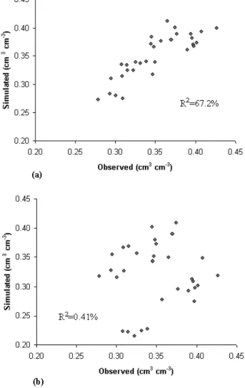
Scatter diagrams of soil water contents for the best (4-parameter, θ + ETa) and the worst (8-parameter, ETa) cases
are shown in Fig. 8a and b. The range in observed soil water contents is limited to wetter conditions (Fig. 8a), so no actual water stress has occurred in the crops. According to Jhorar
Fig. 7. (a) Simulated soil water as compared to the base values using ETa as search criterion (daily, 4-parameter). (b) Simulated soil water as
compared to the base values using ETa as search criterion (weekly, 4-parameter). (c) Simulated soil water as compared to the base values
using ETa as search criterion (daily, 8-parameter). (d) Simulated soil water as compared to the base values using ETa as search criterion
Fig. 8. (a) Scatter diagrams of the best observed and simulated soil water contents after a GA solution in the experimental study
(4-parameter, θ + ETa ). (b) Scatter diagrams of the worst observed and
simulated soil water contents after a GA solution in the experimental
study (8-parameter, ETa )
successful parameter estimation, which is lacking in this case. Ranges in observed ET are from 0.3 to 6.5 mm d-1,
where the lower values do not indicate water stress but are observations at the emergence stage of the crop or after a rainfall event or low evaporative demand (see Figs. 10 and 3). For the worst case (Fig. 8b), the simulated and observed ET values still match reasonably well (Table 1). However, the soil water contents show a big discrepancy between simulated and observed values. This shows that the soil water was not matched properly during the search process; the lower cluster suggests that the soil water was underestimated and the upper cluster along the 45o line
depicts reasonably matched data (see Fig. 9b). But the average error suggests that the prediction improved compared to the case of the 4-parameter problem where ET was used as the criterion (see Table 1). This result reveals
the danger of using only one statistical test criterion in the solutions.
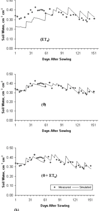
Figure 9a and b show the results of the soil water simulations at the upper soil layer using the derived MVG parameters from the 4- and 8-parameter problems, with the three search criteria being used. In the figures, it is obvious that soil water (θ) as criterion is adequate to define the soil hydraulic parameters because of its direct relationship with the parameters. The case of ET (Fig. 9a), however, is interesting to explore. In theory, for a 4-parameter problem Fig. 9a. Simulated and measured soil water using the GA derived
MVG parameters in the experimental study (4-parameter). ETa
indicates ET alone as criterion, θ, soil water alone and θ + ETa, the
with daily or weekly data, the use of ET as search criterion can define the soil hydraulic parameters adequately. This is true provided that the other (known) parameters are defined properly. Figure 9a shows that the simulated and measured soil water contents using θ as criterion have reasonable agreement with each other, meaning that the other known soil hydraulic parameters defined in this case are quite appropriate. Therefore, the prediction of the soil water using ET as search criterion was influenced by other factor(s) in the process. Along this line, it is speculated that the
uncertainty involved in ET prediction is the main cause of this discrepancy. As observed in Table 1, the R2 of ET did
not change significantly in all cases.
Figure 10 shows the observed ET from the lysimeter (ETlys) and predicted potential ET (ETpot) from the SWAP model. The effect of model and data errors to ETpot can be observed in the figure: there are times in the season when
ETpot values are lower than the ETlys and the unusual opposite trend in some days is apparent.
Discussion
Many studies presented on inverse modelling in the vadoze zone are limited to the so-called forward-backward simulation approach, referred to here as the numerical case. Generated output of a model, with or without artificial random errors, is used as “observed” values in the objective function to estimate the parameters. In most cases results were satisfactory but Jhorar et al. (2002) concluded that parameters were difficult to assess and emphasis should be put on the prediction of the terms considered in the objective function. In this study, the numerical case showed that the GA was able to represent the terms included in the fitness function very well and parameters could be estimated reasonably well, especially if only four parameters were included. It should be taken into account that in this study, periods with water stress are completely lacking, which is considered essential to produce reliable results (Feddes et
al., 1993; Van Dam, 2000; Jhorar et al., 2002). This leads
to the conclusion that the GA approach as used in this study is a powerful tool in inverse modelling.
The cases where the actual lysimeter data were used showed a different picture. Parameter estimations are less successful and the ability of the model to produce similar Fig. 9b. Simulated and measured soil water using the GA derived
MVG parameters in the experimental study (8-parameter). ETa
indicates ET alone as criterion, θ, soil water alone and
ET and soil water values as observed was worse than the numerical case, although the overall performance can be described as reasonable. In reality, better prediction of the actual ET may require parameterisation of the sensitive parameter(s) that can influence the estimate of ET from the simulation model significantly. At the point where GA could not improve the solution any more, the problem could have been controlled already by the model and data errors.
The different performances of the numerical and experimental case indicate clearly the danger of focusing only on the forward-backward approach. Such a numerical approach takes no account of the simplifications, assumptions or errors included in any simulation model. Even the inclusion of a generated random error term in the simulated “observations”, as seen as the ultimate test in many studies, does not overcome this problem. This can be revealed only by the use of real field data.
In addition, GA as a tool is very promising for the inverse problem in the unsaturated zone. Aside from its advantage of partially handling the causes of non-uniqueness and being favourable to highly perturbed functions, the setting up of parameters to be investigated can conveniently be arranged in a series of strings; no complex inversion matrix is required. The concepts of micro and restarting population minimised the problem of the too much redundant fitness function evaluations in a conventional GA and thus improved the computational time. The features of securGA and 90% convergence criterion improved the search for a solution. From other tests, however, convergence criteria lower that 90% did not improve the search; this could be explained by the reduced opportunity of the good genes in an individual being shared and expressed in a generation. For the case of 90% convergence, this disadvantage is compromised by the increased frequency of the fresh influx of new genetic materials. However, a comparison of GA with other methods is highly recommended.
Furthermore, despite the weakness of ET as a criterion in the inverse problem, its use for the practical application at regional scale is appealing because ET is so far the most practical and reliable hydrological component that can be derived from satellite imagery (Bastiaanssen et al., 1998). Setting up the inverse problem appropriately could probably circumvent its weak points. Further research is needed to address this uncertainty.
Acknowledgement
This research has been made possible through the PhD Research Grant awarded to the first author by the International Water Management Institute (IWMI), Colombo, Sri Lanka. Dr. David Carroll of CU Aerospace,
Urbana, IL, USA is acknowledged for his discussions on Genetic Algorithms. The authors are also very grateful to Dr. N.K. Tyagi, Director of the Central Soil Salinity Research Institute (CSSRI), Karnal, Haryana, India for permitting the use of their lysimeter data for this study. The Research Committee at Asian Institute of Technology (AIT), Bangkok, Thailand namely: Prof. Ashim Das Gupta, Assoc. Prof. Rainer Loof, Dr. Roberto Clemente and Dr. Kyoshi Honda are greatly acknowledged for their continued support.
References
Antonopolous, V.Z., 2000. Modeling of soil water dynamics in an irrigated corn field using direct and pedo-transfer functions for hydraulic properties. Irrig. Drainage Syst., 14, 325–342. Bastiaanssen, W.G.M., Menenti, M., Feddes, R.A. and Holtslag,
A.A.M., 1998. A remote sensing energy balance algorithm for land (SEBAL) 1: Formulation. J. Hydrol., 212–213, 198–212. Belmans, C., Wesseling, J.G. and R.A. Feddes., 1983. Simulation of water balance of a cropped soil: SWATRE. J. Hydrol., 63, 271–286.
Black, T.A., Gardner, W.R. and Thurtell, G.W., 1969. The prediction of evaporation, drainage and soil water storage for a bare soil. Soil Sci. Soc. Amer. J., 33, 655–660.
Boesten, J.J.T.I. and Stroosnijder, L., 1986. Simple model for daily evaporation from follow tilled soil under spring conditions in a temperate climate. Neth. J. Agric. Sci., 34, 75–70.
Carroll, D. L., 1996. Genetic Algorithms and optimizing chemical Oxygen-Iodine lasers. In: Developments in theoretical and
applied mechanics, H.B. Wilson, R.C.Batra, C.W. Bert, A.M.J.
Davis, R.A. Schapery, D.S. Stewart and F.F. Swinson (Eds.), Vol. XVIII. School of Engineering, The University of Alabama. 411–424.
Carroll, D. L., 1998. GA Fortran Driver version 1.7. http:// www.cuaerospace.com/carroll/ ga.html
Cieniawski, S. E., Eheart, J. W. and Ranjithan, S., 1995. Using genetic algorithms to solve a multiobjective groundwater monitoring problem. Water Resour. Res., 31, 399–409. Dirksen, C., 1991. Unsaturated hydraulic conductivity. In: Soil
analysis: physical methods, K.A. Smith and C.E. Mullins (Eds.).
Marcel Dekker, New York. 209–269.
Doorenbos, J. and Kassam, A.H., 1979. Yield response to water. Report No. 33. FAO, Rome.
Droogers, P., 1999. PTF: Pedo-transfer function Version 0.1. International Water Management Institute, Colombo, Sri Lanka. Droogers, P., Bastiaanssen, W.G.M., Beyazgül, M., Kayam, Y., Kite, G.W. and Murray-Rust, H., 2000. Distributed agro-hydrological modeling of an irrigation system in Western Turkey. Agric. Water Manage., 43, 183–202.
Feddes, R.A., Kowalik, P.J. and Zarandy, H., 1978. Simulation of
field water use and crop yield: Simulation Monographs. Pudoc,
Wageningen, The Netherlands.
Feddes, R.A., Menenti, M., Kabat, P. and Bastiaanssen, W.G.M., 1993. Is large-scale inverse modeling of unsaturated flow with areal evaporation and soil moisture as estimated from remote sensing feasible? J. Hydrol., 143, 25–152.
Goldberg, D. E. 1989. Genetic algorithms in search, optimization
and machine learning. Addison-Wesley, Reading, Mass.
Hill, M.C., 1992. A computer program (MODFLOWP) for
estimating parameters of a transient, three-dimensional, ground-water flow model using nonlinear regression. U.S. Geological
Holland, J. H., 1975. Adaptation in natural and artificial systems. University of Michigan Press, Ann Arbor.
Jhorar, R.K., Bastiaanssen, W.G.M., Feddes, R.A. and Van Dam, J.C., 2002. Inversely estimating soil hydraulic functions using evapotranspiration fluxes. J. Hydrol. (in press).
Kite, G. and Droogers, P., 2000. Comparing evapotranspiration estimates from satellites, hydrological models and field data. J.
Hydrol., 229, 3–18.
Kool, J.B. and Parker, J.C., 1988. Analysis of the inverse problem for transient unsaturated flows. Water Resour. Res. 24, 817–830. Kool, J.B., Parker, J.C. and Van Genuchten M.Th., 1985.
Determining soil hydraulic properties from one-step outflow experiments by parameter estimation: I. Theory and numerical studies. Soil Sci. Soc. Amer. J., 49, 1348–1354.
Krishnakumar, K., 1989. Micro-Genetic Algorithms for stationary
and non-stationary function optimization. SPIE: Intelligent
Control and Adaptive Systems, Vol. 1196. Philadelphia, PA. Maas, E.V. and Hoffman, G.J., 1977. Crop salt tolerance-current
assessment. J. Irrig. Drain. Eng., ASCE, 103, 115–134. Mualem, Y., 1976. A new model for predicting the hydraulic
conductivity of unsaturated porous media. Water Resour. Res.,
12, 513–522.
Romano, N. and Santini, A., 1999. Determining soil hydraulic functions from evaporation experiments by a parameter estimation approach: Experimental verifications and numerical studies. Water Resour. Res., 35, 3343–3359.
Schaap, M.G., Leij, F.K. and Van Genuchten, M.Th., 1998. Neural network analysis for hierarchical prediction of soil hydraulic properties. Soil Sci. Soc. Amer. J., 62, 847–855.
Šimùnek, J., Wendroth, O. and Van Genuchten, M.Th., 1998. Parameter estimation analysis of the evaporation method for determining soil hydraulic properties. Soil Sci. Soc. Amer. J., 6, 894–905.
Supit, I., Hooyer, A.A. and Van Diepen, C.A. (Eds.), 1994. System
description of the WOFOST 6.0 crop simulation model implemented in the CGMS Vol. 1: Theory and algorithms. EUR
publication 15956, Agricultural series, Luxemberg. 146 pp. Tyagi, N. K., Sharma, D.K. and Luthra, S.K., 2000.
Evapotranspiration and crop coefficients of wheat and sorghum.
J. Irrig. Drainage Eng., ASCE. 126, 215–222.
Van Dam, J.C., Stricker, J.N.M. and Droogers, P., 1992. Inverse method for determining soil hydraulic functions from one-step outflow experiments. Soil. Sci. Amer. J., 56, 1042–1050. Van Dam, J.C., Stricker, J.N.M. and Droogers, P., 1994. Inverse
method for determining soil hydraulic functions from multistep outflow experiments. Soil. Sci. Amer. J., 58, 647–652.
Van Dam, J.C., Huygen, J., Wesseling, J.G., Feddes, R.A., Kabat, P., Van Waslum, P.E.V., Groenendjik, P. and Van Diepen, C.A., 1997. Theory of SWAP version 2.0: Simulation of water flow
and plant growth in the Soil-Water-Atmosphere-Plant environment. Technical Document 45. Wageningen Agricultural
University and DLO Winand Staring Centre, The Netherlands. Van Dam, J.C., 2000. Field-scale water flow and solute transport.
SWAP model concepts, parameter estimation and case studies.
Doctoral Thesis. Wageningen University. The Netherlands. Van Genuchten, M.Th., Leij, F.J. and Yates, S.R., 1991. The RETC
code for quantifying the hydraulic functions of unsaturated soils.
Robert S. Kerr Environmental Research Laboratory, U.S. Environmental Protection Agency, Oklahoma, USA. 83 pp. Van Genuchten, M.Th., 1980. A closed form equation for
predicting the hydraulic conductivity of unsaturated soils. Soil
Sci. Soc. Amer. J., 44, 349–386.
Vereecken, H., Maes, J., Feyen, J. and Darius, P., 1989. Estimating the soil moisture retention characteristic from texture, bulk density and carbon content. Soil Sci., 148, 389–403.
Vereecken, H., Maes, J. and Feyen, J., 1990. Estimating unsaturated hydraulic conductivity from easily measured properties. Soil Sci., 149, 1–12.
Watermark Computing, 1994. PEST: model independent
parameter estimation. Watermark Computing, Brisbane,
Australia.
Wösten, J.H.M., Lilly, A., Nemes, A. and Le Bas, C., 1998. Using
existing soil data to derive hydraulic parameters for simulation models in environmental studies and in land use planning.
Report 156. DLO Winand Staring Centre, The Netherlands. Xevi, E., Gilley, J. and Feyen, J., 1996. Comparative study of two
crop yield simulation models. Agric. Water Manage., 30, 155– 173.
Yang, G., Reinstein, L.E., Pai, S., Xu, Z. and Carroll, D.L., 1998. A new genetic algorithm technique in optimization of permanent 125-I prostate implants. Med. Phys., 25, 2308–2315.
Yeh, W.W-G., 1986. Review of parameter identification procedures in groundwater hydrology: The inverse problem.
Water Resour. Res., 22, 95–108.
Zheng, C., 1997. ModGA_P: Using Genetic Algorithms for
parameter estimation. Technical Report to DuPont Company,
Hydrogeology Group, University of Alabama, USA.
Zurmühl, T. and Durner, W., 1998. Determination of parameters for bimodal hydraulic functions by inverse modeling. Soil Sci.