Dual lidar observations of mesoscale fluctuations of ozone and horizontal winds

HAL Id: insu-03087746

https://hal-insu.archives-ouvertes.fr/insu-03087746

Submitted on 24 Dec 2020

HAL is a multi-disciplinary open access

archive for the deposit and dissemination of

sci-entific research documents, whether they are

pub-lished or not. The documents may come from

teaching and research institutions in France or

abroad, or from public or private research centers.

L’archive ouverte pluridisciplinaire HAL, est

destinée au dépôt et à la diffusion de documents

scientifiques de niveau recherche, publiés ou non,

émanant des établissements d’enseignement et de

recherche français ou étrangers, des laboratoires

publics ou privés.

Dual lidar observations of mesoscale fluctuations of

ozone and horizontal winds

D. Gibson-Wilde, R. Vincent, Claude Souprayen, Sophie Godin, Albert

Hertzog, S. Eckermann

To cite this version:

D. Gibson-Wilde, R. Vincent, Claude Souprayen, Sophie Godin, Albert Hertzog, et al.. Dual lidar

observations of mesoscale fluctuations of ozone and horizontal winds. Geophysical Research Letters,

American Geophysical Union, 1997, 24 (13), pp.1627-1630. �10.1029/97GL01609�. �insu-03087746�

Dual lidar observations of mesoscale fluctuations

of ozone and horizontal winds

D. E. Gibson-Wilde and R. A. Vincent

Department of Physics and Mathematical Physics, University of Adelaide, S.A. 5005, Australia

C. Souprayen,

S. Godin, and A. Hertzog

S. D. Eckermann 1

Computational Physics, Inc., Fairfax, Virginia 22031

Abstract. A case study is presented of 6.5 h of simulta- neous colocated stratospheric Differential Absorption Lidar

(DIAL) measurements of ozone concentration and Rayleigh-

Mie Doppler (RD) lidar measurements of horizontal wind velocity from the Observatoire de Haute Provence (OHP),

France (44øN, 6øE). The RD lidar observations reveal a dis-

tinct gravity wave motion at •12-18 km, while the DIAL

data show laminated ozone structures in the same height

range. We combine these data to show that advection due to the gravity wave cannot produce the large ozone lamina at

•14 km.

Introduction

Stratospheric ozone abundances exhibit appreciable meso- scale variability. Large perturbations with vertical scales • 1-5 km are observed routinely in ozonesonde data [Ehhalt et al., 1983; Hofmann et al., 1989; Reid and Vaughan, 1991;

Teitelbaum et al., 1994; Mitchell et al., 1996], while mea-

surements from stratospheric aircraft show variability over a broad range of horizontal scales [Nastrom et al., 1986;

Danielsen et al., 1991; Bacmeister et al., 1996]. Since ozone

in the lower stratosphere (below •25 km) is photochemically inactive on timescales up to 5 days (in the absence of hetero- geneous processing), then such variability must in general

have a dynamical origin.

Gravity-wave-induced vertical advection was first sug- gested as a possible cause of ozone perturbations by Chiu and Ching [ 1978]. Aircraft observations during the Stratosphere- Troposphere Exchange Project (STEP) revealed inertia-grav- ity waves (IGWs) and seemingly related perturbations of

ozone and other constituents [Chan et al., 1991; Wilson et al.,

1991; Alexander and Pfister, 1995]. Danielsen et al. [ 1991 ] argued that the vertical and horizontal displacements of these IGWs produced the observed ozone perturbations, and that irreversible constituent transport resulted as these waves dis- sipated. Teitelbaum et al. [1994], Alexander and Pfister [ 1995] and Teitelbaum et al. [ 1996] argued that gravity-wave-

induced vertical advection accounted for the ozone fluctua-

tions in their data.

Conversely, Ehhalt et al. [ 1983] found that long-term vari-

ances of ozone inferred from ozonesonde releases at Hohen-

peissenberg (47ø N, 11 o E) were significantly larger than those expected on the basis of wave-induced potential temperature fluctuations alone, indicating that gravity wave vertical ad- vection cannot explain all of the structure. Later analysis of variability in a large base of ozonesonde data from middle to high northern latitudes by Reid et al. [1993] identified the largest perturbations (so-called "laminae") with differen- tial transport across the polar vortex edge. High-resolution parcel advection models of this transport have succeeded in simulating laminated vertical ozone profiles which are sim- ilar to those observed [e.g., Orsolini et al., 1995]. Indeed,

Newman and Schoeberl [ 1995] recently used such a model to

argue that quasi-horizontal flow in and out of the polar vor- tex could explain those laminar ozone structures observed in STEP data which Danielsen et al. [1991] had previously at- tributed to IGW motions. Recent analysis of a large amount of airborne stratospheric ozone data by Bacmeister et al. [1996] concluded that neither IGWs nor large-scale advec- tion alone could explain the mean mesoscale variability ev- ident in these data, and that both effects may combine and interact to produce the observed variability.

Recent studies by Reid et al. [1994] and Langford et al. [ 1996] combined velocity and ozone data to investigate IGW activity in ozone. However the poor temporal resolution of sonde data was a limiting factor in the study of Reid et al. [1994] and the spatial separation of 75 km of the radar and DIAL instrument in the experiments of Langford et al.

[1996] meant that waves observed in one data set may not always relate to those in the other. Here, we report on a

pilot experiment which was devised to avoid many of these

difficulties. Two colocated lidar instruments were used to

acquire simultaneous stratospheric velocity and ozone data with high vertical and temporal resolution. We use these velocity data to identify and characterize an IGW in the stratosphere and to predict its effect on ozone profiles, then compare these predictions with the contemporaneous ozone data to infer the processes responsible for the structure in the ozone data.

•also c/o E. O. Hulburt Center for Space Research, Code 7641,

Naval Research Laboratory, Washington, D.C. 20375 Observations Copyright 1997 by the American Geophysical Union.

Paper number 97GL01609.

0094-8534/97/97 GL-01609505.00

The DIAL ozone and RD lidars, located approximately

10 m apart within the same building at OHP, were run si- multaneously during the observation period (2230 LT on 23

October to 0500 LT on 24 October, 1995). Table 1 sum-

1628 GIBSON-WILDE ET AL.: MESOSCALE OZONE FLUCTUATIONS

Table 1. DIAL and RD lidar capabilities at OHP.

Ozone DIAL RD lidar

Beam vertical vertical + off-zenith

direction 40 ø north and east Wavelengths absorbed 308 nm 532 nm

reference 355 nm

PRF 50 Hz 30 Hz

Height resol. 600 m 115 m

Time resol. 30 min 30 min

Height range 12- 30 km 12 -45 km Major error water vapour aerosols

sources aerosols

marizes the operational specifics of both lidar systems (see

also Garnier and Chanin [1992] and Lacoste et al. [1992]). •

Measurements of lower stratospheric (12-30 km) ozone con- centration were provided by the DIAL system and zonal and meridional velocities were provided by the RD lidar.

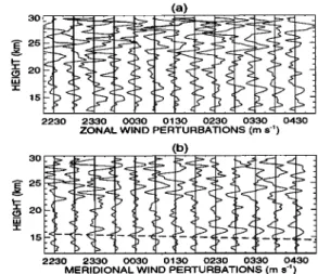
Figure 1 presents the sequence of DIAL ozone concentra- tion profiles in two consecutive plots. The estimated error in measurement is •10% in the height range 12-20 km. The RD lidar zonal and meridional velocity profiles in Figure 2 are displayed at a vertical grid spacing of 150 m, obtained from regridding using spline interpolation from the initial

115 m resolution, for compatibility with the DIAL profiles. The RD lidar data are acquired typically with a time resolu- tion of 5 min so that the 30 min profiles presented here have an estimated error of less than 5% between 12-20 km.

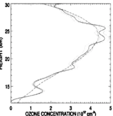
Figure 3 displays the average ozone concentration profile calculated over the 6.5 h observation period. The error asso- ciated with this average profile is •2% in the height range

12-20 km. The small-scale features evident in this average

profile must result from dynamical activity on timescales greater than 6.5 hours.

Ozone Laminae

The two local maxima in ozone concentration in Figure 3 at • 14 km and • 18 km are examples of ozone laminae. They were identified as such using the definition of Reid and Vaughan [1991] which requires large positive or negative

ozone concentrations which are limited to a layer less than

3O 25 20 15 2230 2330 0030 0130 OZONE CONCENTRATION (1012 cm '3) 25 20 15 0200 0300 0400 0500 OZONE CONCENTRATION (1012 cm '3)

Figure 1. DIAL ozone concentration profiles from 2230

LT on 23 October to 0500 LT on 24 October, 1995. Each

profile is labeled by the start time of its 30 min integration.

Successive

profiles

are

offset

by 5x 1012cm

-3.

3O • 25 3O • 25 (a) 2230 2330 0030 0130 0230 0330 0430

ZONAL WIND PERTURBATIONS (m s '1) (b)

2230 2330 0030 0130 0230 0330 0430

MERIDIONALWIND PERTURBATIONS (m s '1)

Figure 2. RD lidar profiles from 2230 LT on 23 October to 0500 LT on 24 October, 1995. The zero point of each profile is labeled with the starting time of its 30 min observational

integration.

Successive

profiles

are

offset

by 10 m s

-].

2.5 kmin vertical extent. Reidand Vaughan [ 1991 ] found that the majority of laminae in mid-latitude, northern hemispheric

ozonesonde data were within the height range 12-18 km.

The 6.5 h mean lidar ozone concentration profile (Figure 3) was compared with an ozone concentration profile from an ozonesonde launched from OHP at 1200 LT on 24 October

1995, 7 h after the final lidar profile (not shown here). The ozonesonde profile confirmed the lidar observation of the

lamina at 14 km so that a minimum lifetime of 14 h was estimated for the lamina at 14 km based on its occurrence in

both the lidar and ozonesonde profiles. The lamina at 18 km was reduced by the time of the ozonesonde flight. Thus, from

the lidar observations alone, the estimated minimum lifetime

for the 18 km lamina was 6.5 h.

An Inertia Gravity Wave

Successive vertical profiles of zonal and meridional ve- locities from the RD lidar (Figure 2) indicate a wave-like feature below 20 km with downward phase (upward energy) propagation which persists throughout the 6.5 h observation period. A hodograph analysis (Figure 4) shows mostly clock-

wise rotation of the velocity fluctuations with height and a

well-defined velocity ellipse, which suggests that this feature is a long-period upward-propagating IGW. The wave param- eters were derived from these data using a Stokes parameter analysis [e.g., Eckermann, 1996] and are presented in Table 2. The values of observed and intrinsic wave frequency were used to infer that the horizontal propagation direction of the IGW was towards the south-west.

Vertical IGW Displacements

The IGW parameters in Table 2 were used to estimate the

influence of vertical advection due to this IGW on the ozone concentration profile. For adiabatic motion and a constant

background ozone gradient, the relative ozone concentration perturbation, O•/O3, is given by [Chiu and Ching, 1978]

25 ':*'•""' ..'- "!

•2o

..-;•.-.,'""

' -'

15

,

0 1 2 3 4 5

OZONE CONCENTRATION (10 •2 cm '3)

Figure 3. Mean 6.5 h profile of ozone concentration (bold line) and fitted mean profile (dashed-dotted line). A 5% error

estimate is indicated by the dotted line.

where

iUt(z'

t) 6]_/2(c•) (2)

½'(z,

t) =

is the vertical displacement of a parcel by the IGW, & is in-

trinsic

frequency,

6_ (&) - 1 - (f/&)2, f is the inertial

fre-

quency, U•(z, t) is the horizontal velocity perturbation along

the wave

vector,

03(z) is the

background

ozone

concentra-

tion (assumed time-invariant), H is the pressure scale height, ? is the ratio of specific heats (• 1.4), and N is the Brunt-

V'fiis•il[i

frequency

(•0.02 rad s- ] based

on ozonesonde

tem-

perature

data).

The 03(z) profile

was

estimated

by a low-

pass filtered cubic polynomial fit to the mean profile, which removes the laminae (see Figure 3).

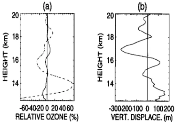
Figure

5a shows

the measured

O•(z, t)/O3(z) deviations

from the cubic polynomial-fitted profile, as well as the expected perturbation produced by the IGW in Figure 4, calculated by first converting U'(z, t) to a •'(z, t) oscilla- tion using_(2) (see Figure 5b), then using this to calculate O•(z,t)/O3(z) using (1). The relative magnitudes of the measured and calculated ozone perturbations in Figure 5a show that the vertical advection produced by the IGW in Figure 4 can drive only a 5% relative ozone fluctuation, ex- cept in the height_region below • 14.5 km where the inverse dependence on O3(z) in (1) leads to perturbations of up to 10%. The estimation of 03(z) using the smoothed profile with laminae removed is the key factor in this calculation,

Table 2. IGW parameters derived from successive RD

lidar profiles and Stokes parameters analysis.

Wave Parameter Estimated Value Vertical wavelength

Observed vertical phase speed Observed frequency Intrinsic frequency Horizontal wavelength 2.3 km -0.06 m s-] 1.6f ,-• 0.00016 rad S --1 2.2f • 0.00022 rad s -1 360 km

and gives the expected response in the absence of preexist- ing ozone lamination. Figure 5 clearly illustrates that the lamina at 14 km cannot result from vertical advection by the

coexisting IGW in Figure 4. Horizontal IGW Displacements

Horizontal IGW displacements were neglected in (1) be- cause the lidar data do not provide information on mean _

horizontal gradients in 03. However, when zonal and merid-

ional

03 gradients

are

nonzero,

additional

contributions

to (1)

arise due to the zonal (X •) and meridional (•b •) displacements

of the wave [e.g., Danielsen et al., 1991]. Since the IGW

propagates south westward, with & •2.2f and U • peaking at

,-04

m s- ], then

X • and

•b

• both

oscillate

air parcels

4-12.7

km

zonally and meridionally from their equilibrium positions. For horizontal IGW displacements to produce the lamina at 14 km, large increases in 03 must occur no more than •20 km away from the lidar sit• so that the IGW can advect these larger ozone abundances into (and then out of) the lidar field-of-view. This also means that such an IGW-produced lamina could exist over a given location for no longer than one ground-based period of the wave, which from Table 2

is • 10.8 h. Since the lamina at 14 km was observed to be

stable over at least 14 h, it is clear that horizontal advection

due to the IGW cannot explain this feature.

Since advection by the IGW cannot produce the observed lamina at 14 km, this strongly suggests that it resulted from synoptic-scale advection patterns. Initial indications from isentropic parcel advection calculations suggest that a fila- mentary structure was indeed present at approximately 14 km over OHP during this experiment [R.J. Atkinson, private com- munication]. The lamina at 18 km appeared to vary in shape and intensity from profile to profile (see Figure 1). Con- sequently, IGW-induced horizontal advection could play a more significant role in driving this feature.

, , , ! i , , , i , , ,

-2 O 2 4

ZONAL WIND PERTURBATIONS (m s -•)

Figure 4. Hodograph between 12-20 km of mean 6.5 h zonal

and meridional wind fluctuations smoothed over 600 m. The

bold line is the major axis of the gravity-wave ellipse from the Stokes parameters analysis.

Conclusions

The dual lidar measurement technique described here per- mits a more thorough study of mesoscale dynamics and tracer variability than has been possible previously. The RD lidar data revealed an upward-propagating IGW below 20 km, with a vertical wavelength of 2.3 km, an observed vertical

phase

speed

•0.06 m s -•, and a peak

horizontal

velocity

amplitude

of ~4 m"s

-• . We were

able

to show

conclusively

that the strength and pers•istence of an ozone lamina at 14 km in DIAL data, was not explained by wave advection. Con- versely, the observed variability of a lamina at 18 km was

somewhat more consistent with IGW influences.

The time-height coverage and resolution of both data sets were vital in allowing us tO form these conclusions. Further observations using this technique should be especially valu- able in investigating gravity waves, filamentary ozone struc- tures, and their interactions, which Bacmeister et al. [ 1996]

1630 GIBSON-WILDE ET AL.: MESOSCALE OZONE FLUCTUATIONS

20•

...

,

...

20

.'

•' 18 ,' '

•' 18

2

• 16

RELATIVE OZONE (%) VERT. DISPLACE. (m) Figure 5. Measured relative ozone concentration pertur- bation determined by subtracting a cubic polynomial mean profile (dotted-dashed curve in panel (a)) and calculated re- sponse of the IGW using (1) and (2) (solid curve in panels (a) and (b), respectively).

have argued may be very important in explaining observed power spectra of ozone variability in the lower stratosphere.

Acknowledgments. We thank the OHP staff and Dr. R. Atkin-

son of BMRC, Melbourne, for useful comments. DGW acknowl- edges University of Adelaide support to visit CNRS.

References

Alexander, M. J., and L. Pfister, Gravity wave momentum flux in the lower stratosphere over convection, Geophys. Res.

Lett., 22, 2029-2032, 1995.

Bacmeister, J. T., S.D. Eckermann, P. A. Newman, L. Lait, K. R.

Chan, M. Loewenstein, M. H. Profitt, and B. L. Gary, Strato- spheric horizontal wavenumber spectra of winds, potential tem-

perature and atmospheric tracers observed by high-altitude air-

craft, J. Geophys. Res., 101, 9441-9470, 1996.

Chan, K. R., S.G. Scott, S. W. Bowen, S. E. Gaines, E. F.

Danielsen, and L. Pfister, Horizontal wind fluctuations in the

stratosphere by internal waves of short vertical wavelength, J.

Geophys. Res., 96, 17,425-17,432, 1991.

Chiu, Y. T, and B. K. Ching, The response of atmospheric and lower ionospheric layer structures to gravity waves, Geophys.

Res. Lett., 5, 539-542, 1978.

Danielsen, E. F., R. S. Hipskind, W. L. Starr, J. F. Vedder, S. E.

Gaines, D. Kley, and K. K. Kelly, Irreversible transport in the stratosphere by internal waves of short vertical wavelength, J.

Geophys. Res., 96, 17,433-17,452, 1991.

Eckermann, S. D., Hodographic analysis of gravity waves: Rela- tionships among Stokes parameters, rotary spectra, and cross-

spectral methods, J. Geophys. Res., 101, 19,169-19,174, 1996.

Vhhalt, D. G., E.P. Roth, and U. Schmidt, On the temporal vari-

ance of stratospheric gas concentrations, J. Atmos. Chem., 1, 27- 51, 1983.

Gamier, A., and M. L. Chanin, Description of a Doppler Rayleigh LIDAR for measuring winds in the middle atmosphere, App.

Phys. B, 55, 35-40, 1992.

Hofmann, D. J., J.W. Harder, J. M. Rosen, J. V. Here-

ford, and J. R. Carpenter, Ozone profile measurements at Mc-

Murdo Station, Antarctica, during the spring of 1987, J. Geophys.

Res., 94, 16,527-16,536, 1989.

Lacoste, A.M., S. Godin, and G. Megie, Lidar measurements and Urnkehr observations of the ozone vertical distribution at the Observatoire de Haute Provence, J. Atmos. Terr. Phys., 54, 571- 580, 1992.

Langford, A. O., M. H. Proffitt, T E. VanZandt, and J.-F. Lamar-

que, Modulation of tropospheric ozone by a propagating gravity

wave, J. Geophys. Res., 101, 26,605-26,613, 1996.

Mitchell, N.J., A.J. McDonald, S. J. Reid, and J. D. Price,

Observations of gravity waves in the upper and lower stratosphere

by lidar and ozonesondes, Ann. Geophys., 14, 309-314, 1996. Nastrom, G. D., W. H. Jasperson, and K. S. Gage, Horizon-

tal spectra of atmospheric tracers measured during the Global Atmospheric Sampling Campaign, J. Geophys. Res., 91, 13,201-

13,209, 1986.

Newman, P. A., and M. R. Schoebed, A reinterpretation of the data from the NASA Stratosphere-Troposphere Exchange

Project, Geophys. Res. Lett., 22, 2501-2504, 1995.

Orsolini, Y., P. Simon, and D. Cariolle, Filamentation and layering

of an idealized tracer by observed winds in the lower strato- sphere, Geophys. Res. Lett., 22,839-842, 1995.

Reid, S.J., and G. Vaughan, Lamination in ozone profiles in the

lower stratosphere, Q. J. R. Meteorol. Soc., 117, 825-844, 1991.

Reid, S. J., G. Vaughan, and E. Kyro, Occurrence of ozone laminae

near the boundary of the stratospheric polar vortex, J. Geophys.

Res., 98, 8883-8890, 1993.

Reid, S.J., G. Vaughan, N.J. Mitchell, I. T Prichard, H. J. Smit, T. S.

Jorgensen, C. Varotsos, and H. de Backer, Distribution of ozone

laminae during EASOE and the possible influence of inertia-

gravity waves, Geophys. Res. Lett., 21, 1479-1482, 1994.

Teitelbaum, H., J. Ovafiez, H. Kelder, and F. Lott, Some

observations of gravity-wave-induced structure in ozone and water vapour during EASOE, Geophys. Res. Lett., 21, 1483-

1486, 1994.

Teitelbaum, H., M. Moustaoui, J. Ovafiez, and H. Kelder, The role

of atmospheric waves in the laminated structure of ozone profiles

at high latitudes, Tellus, 48A, 422-455, 1996.

Wilson, J. C., W. T. Lai, and S. D. Smith, Measurements of

condensation nuclei above the jet stream: Evidence for cross jet

transport by waves and new particle formation at high altitudes, J.

Geophys. Res., 96, 17,415-17,423, 1991.

Dorothy Gibson-Wilde and Robert Vincent, Department of Physics and Mathematical Physics, University of Adelaide, 5005,

Australia. (e-mail: [email protected])

Claude Souprayen, Sophie Godin, and Albert Hertzog, Service

d'Aeronomie, CNRS, France.

Stephen Eckermann, Computational Physics, Inc., Fairfax, Virginia. (e-mail: [email protected])