Development of the kinematic model for an ultrasound scanning machine by means of dual quaternion transformations of screw coordinates

11, 11il 1 j 111

3 9080 00580040 1

DEVELOPMENT OF THE KINEMATIC MODEL FOR AN

ULTRASOUND SCANNING MACHINE BY MEANS OF

DUAL QUATERNION TRANSFORMATIONS OF SCREW

COORDINATES

by

SCOTT EDWARD SCHWARTZ SUBMITTED TO THE DEPARTMENT OF

MECHANICAL ENGINEERING

IN PARTIAL FULFILLMENT OF THE REQUIREMENTS FOR THE DEGREE OF

BACHELOR OF SCIENCE IN MECHANICAL ENGINEERING

at the

MASSACHUSETTS INSTITUTE OF TECHNOLOGY May 1989

@

Massachusetts Institute of Technology 1989

Signature

Signature o

Certified by

Redacted

f Author

Departn t of Mechanical Engineering

Signature Redacted

May 12, 1989

Professor Robert W. Mann

Signature Redacted

Thesis Supervisor

Accepted by

Professor Peter Griffith Chairman, Department Committee

DEVELOPMENT OF THE KINEMATIC MODEL FOR AN UTRASOUND SCANNING MACHINE BY MEANS OF DUAL QUATERNION TRANSFORMATIONS OF SCREW COORDINATES

by

SCOTT EDWARD SCHWARTZ

Submitted to the Department of Mechanical Engineering on May 12, 1989 in partial fulfillment of the requirements for the Degree of Bachelor of Science in

Mechanical Engineering ABSTRACT

Dual quaternion transformations based on screw coordinates were used to develop the kinematic model for a bifurcated ultrasound scanning machine. Screw representa-tion was found to be the most efficient and simple method of defining relative posirepresenta-tions of links and joints in an open loop kinematic chain. A simple example is given to verify that the technique produces accurate results. Two methods, a computer mathematical package and an iterative nonlinear program, were used to solve the trajectory problem for the bifuraceted scanner. The mathematical package was unable to handle the com-plicated kinematic equations and obtain a closed form solution. The iterative program was developed to solve the trajectory problem for a given move.

Thesis Supervisor: Professor Robert W. Mann

Title: Whitaker Professor of Biomedical Engineering Department of Mechanical Engineering

Co-Thesis Supervisor: Mike C. Murphy Title: Doctoral Student

Acknowledgements

I would like to thank Mike Murphy for his guidance, support and encouragement.

Thanks to Mary and Elliot, my parents, for their constant support thoughout my life.

And Nancy, for her support and love.

This thesis project was conducted in the Eric P. and Evelyn E. Newman Labo-ratory for Biomechanics and Human Rehabilitation in the Department of Mechanical Engineering at the Massachusetts Institute of Technology.

Table of Contents

Abstract

1

Acknowledgements

2

Table of Contents

3

List of Figures

4

List of Tables

5

1 Introduction

6

2 Background

8

2.1 Screw Coordinates ...

8

2.2 Transform ations ...

10

2.3 Quaternion Transformations Between Lines ...

11

2.4 Screw Representation of Links and Pairs ...

13

2.5 The Kinematics of a Simple Manipulator ...

16

3 Kinematic Model

20

4 Trajectory Planning Algorithm

28

4.1 M athem atica

... 29

4.2 Iterative Programming Method

... 31

5 Conclusion

32

List of Figures

2.1 G eneral spatial triangle ... 12

2.2 A generalized link in a spatial mechanism

illustrating the parameters used to define

orientation and position of lines in space ...

13

2.3 Symbolic representation of a revolute pair ...

14

2.4 Symbolic representation of a prismatic pair ...

15

2.5 A simple two degree-of-freedom manipulator ...

16

2.6 Symbolic representation of kinematic chain of two

degree-of-freedom manipulator using screw representation ...

17

3.1 Relative orientation of kinematic pairs

in the bifurcated scanning application ...

21

3.2 Symbolic representation of the kinematic chain

of the scanning m achine ...

23

List of Tables

2.1 A summary of parameters and notation

for revolute and prismatic pairs ...

15

2.2 Manipulator link and pair parameters ...

18

3.1 Model and parameters for scanner joints ...

22

3.2 Scanner link and pair parameters ...

24

Chapter 1

Introduction

Extensive research is being conducted in the field of biomechanics to develop a mathe-matical model of the human musculoskeletal system. One of the important areas of this research is aimed the at development of a kinematic model of the knee joint. Obtaining accurate three dimensional geometric mapping of the bone and cartilage surface of this synovial joint is essential to the development of the kinematic model. Traditionally, the geometric contours have been measured using destructive techniques such as serial slicing

[16].

This technique alters the natural state of the bone and cartilage which can introduce errors in the measurements. Recently, the geometric contours of the joint have been determined using techniques such as computer tomography [8], stereopho-togrammetry [1], and pulse-echo ultrasound [12]. These techniques employ non-invasive measuring systems that produce geometric contour measurements of differing accuracy. The pulse ultrasound has been shown to produce the most precise contour measure-ments of the bone and cartilage surfaces. However, thus far this technique has been limited to the measurement of the hip joint which has a near spherical surface. Contour measurements of the knee joint require a more versatile scanning setup.

Currently in the Newman Laboratory for Biomechanics and Rehabilitation at MIT, a project is in progress to develop a scanning system that will be able to scan general surfaces. An ultrasound system that will utilize two independent kinematic branches

for the positioning of the scanning transducer was developed [7]. This machine will enable the scanning of a general surface such as the knee joint surfaces. This system also provides faster, more accurate positioning of the ultrasonic beam. Seering has developed a similar robot manipulator that is a combination of a two- and a four-degree-of-freedom manipulator systems working in parallel [13]. This configuration is seen as the future in precision robotics because of the increased speed, accuracy and stiffness that are gained. However, this bifurcated setup complicates the trajectory control of the machine.

This paper presents the formulation of the kinematic model and trajectory planning algorithm for the ultrasound scanning machine. Traditionally, a point transformation scheme would be used to control the scanner. In ultrasound scanning, it is important to position the axis of the transducer perpendicular to the surface being scanned. This enhances geometrical accuracy and is essential if the returned sound energy is used to estimate cartilage modulus. Thus, line tranformations are more applicable for the development of the kinematic model.

The scanner allows for general surface measurements by simply aligning the trans-ducer beam with the normal vector to a surface. In this thesis, line transformations based on screw coordinate representation are used to model the kinematic pairs and links of the scanning machine. Screw coordinates with a geometry based on lines are a convenient way to descibe kinematic pairs. Using the techniques of dual quater-nion transforms which Yang [18] developed to describe closed loop mechanisms, the equations describing the position of the transducer beam and normal surface line were developed. A commercial mathematical computer package was utilized to simplify and solve the complicated equations which described the motion of the machine.

This paper divided into three parts. Chapter 2 gives a brief overview of screw notation, mathematics and transformations used in the thesis. The kinematic model is developed and presented in Chapter 3. A description of two techniques that were used to solve the trajectory problem is presented in Chapter 4.

Chapter 2

Background

2.1

Screw Coordinates

Most manipulators are controlled by using a matrix based homogeneous point transfor-mation scheme [9]. The general opinion is that point transfortransfor-mations provide a reliable and tested method for describing the motion of a manipulator. Computers are also able to manipulate the matrices in a straight forward fashion. However, it is difficult to achieve closed form solutions for real time computation of displacements and ve-locities by this method because the homogeneous coordinates of points only provide information about the location of points [15]. Screw representation provides the means to describe the general motion of a rigid body. Chasles demonstated that the most general displacement of a rigid body in three-dimensional space is a combination of a rotation about and a translation along a line [6]. Screw coordinates, therefore, pro-vide a general representation of the motion of links in a mechanism allowing for easy computation of the finite and instantaneous motion of the specific links. Yang [18] and Yuan and Freudenstein [19,20] used projective transformations of screw coordinates for the analysis of spatial mechanisms and linkages. Sugimoto [15] described the kinematic analysis of manipulators by means of screw coordinates. Although highly encouraged by researchers such as Roth [11], the application of screw representation in the

devel-opment of kinematic models for manipulators is limited. In the case of the ultrasound scanning machine, the screw transformations are highly relevant because of the need to align lines in space.

The basics of screw coordinates and screw calculus were first introduced by Ball

(2].

A screw is a line in space which has an associated magnitude. This screw can be represented by six coordinates; three of the coordinates consist of the components of the vector which define the direction of the screw (L, M, N), and the other three coordinates consist of the components of the vector which define the moment of the line about the origin (L,, M, N,). The screw can, therefore, be defined as:

(L, M, N, Lo, M, No) (2.1)

The screw can be written in the dual number form. A dual number can be expressed as [4]:

a = a + Ea0 (2.2)

where a and ao are real numbers and e2

= 0. Similarly, a screw X can be expressed in the dual notation form as:

X = X + EX0 (2.3)

where X and X, are vectors with the respective components given in eqn.(2.1). There-fore, the dual screw is defined as:

(L, M, N) + E(LO, M, N) (2.4)

It is also convenient to use a screw to define general rigid body motion. Motion of a rigid body is constrained by a line in space which is defined by four parameters. Displacement from point A to point B will consist of a translation along the line, S, and a rotation about that line, 0. This screw displacement can be described using dual notation as a dual angle by:

2.2

Transformations

There are several types of transformations that can be used to define rigid body motion. Rooney presents a comparison of eight methods of representing a general spatial screw displacement, concluding that the dual unit quaternion is the best method for line transformation [10]. The quaternion which consists of four paremeters was originally developed by Hamilton [5] to represent rigid body rotation. The need to represent general screw diplacement led to the development of the dual quaternion by Clifford

[4].

A dual quaternion is basically a mix of quaternion and dual number. The dual quaternion is composed of a 4-tuple of dual numbers.

q = (a + ca., b + Eb,, c + Eco, d + Edo) (2.6)

This can be expressed in dual form as:

q = (a, b, c, d) + E(a., bo, _co, do) = q + cqo (2.7)

where q and q, are real quaternions. The dual quaternion can also be expressed in terms of the vector quantities (i, j,k):

q = (a + Eao) + (b+ ebo)i+ (c + Ec,)j+ (d + Edo)k (2.8)

It can be seen that the dual quaternion is composed of a scalar part Sq, and a vector part Vq^. The multiplication of two dual quaternions q and A turns out to be simply:

AA =VAx V^ j-V-V P+SA*Vf +S *VA-+ S?*S (2.9)

Yang first applied the transformation of line coordinates in the form of dual quater-nions to the analysis of closed loop mechanisms

[18].

The dual quaternion transforma-tion is more efficient than the conventransforma-tional matrix transformatransforma-tion. The transformatransforma-tion between two screws in space in matrix notation turns out to be a 6 x 6 array [19,20. Although matrix manipulations can be implemented effectively on a computer system,

the size of the matrix creates large computational inefficiencies. Nine of the compo-nents in the matrix are always zero while an additional nine compocompo-nents are the same. Therefore, redundant and unnecessary multiplications occur.

Dual quaternions have the advantage of requiring definition of only eight real num-bers. Considering that only four numbers are needed to represent a line in space, the eight components of the quaternion are the minimum number needed to represent the transformation between two lines in space. Dual quaternion multiplication consists of 96 multiplies whereas 216 multiplies are needed using conventional 6x6 matrices. Given the fact that a significant number of the matrix multiplies are with zero, the dual quaternion provides a more efficient representation of line transformations. In a comparison of different representations of line transformation, Rooney [101 found that dual quaternions were the best way to represent line transformation because of their simplicity and economy.

2.3

Quaternion Transformations Between Lines

To develop the quaternion transformation between lines in space consider Figure 2.1, which is a closed loop configuration of three non-intersecting and non-parallel lines in space producing a spatial triangle. The three lines, S*,

S2;,

51*, are connected by three

mutually perpendicular lines, a12, a₂₃, a&l. Dual angles specify the relative position of the lines and the common perpendiculars.

Consider the transformation between S* and S* with a* as the mutual perpendic-ular between the two line vectors. Define a12 as a12 + Ea1 where a12 is the projected

angle and a1 2 is the length of the common perpendicular between S* and S2*. Define 01

as 0₁ + ES1 where

E

1 is the projected angle between 8* and a2' and S, is the distance

along * to a12. The transformation between the two line vectors is:

S aa

Figure 2.1: General spatial triangle illustrating the parameters used to define orienta-tion and posiorienta-tion of lines in space [18].

where

Q2 = cos(& 2) + a*2sin(a1 ) (2.11)

It should be noted that this form of the transformation holds only for the case where the line a*2 is perpendicular to both Sj* and S*- Similarily, the relationship between sucessive mutual perpendiculars between the two vector lines is:

12 = Q1^* (2.12)

where

Q1 = COS(e 1) + S1*sin(01 ) (2.13)

Therefore, the transformation between sucessive line vectors in space is defined by dual angles that specify the relative position of the vectors in space. This relation-ship between lines can be compactly represented symbolicly using the dual quaternion notation.

Figure 2.2: A generalized link in a spatial mechanism (181.

2.4

Screw Representation of Links and Pairs

Using screw representation, the motion of kinematic pairs can be described. Prismatic joints are constrained by the line of translation whereas revolute joints are constrained by the axis of rotation. Denavit and Hartenberg developed a kinematic notation based on matrices to describe lower-pair mechanisms

[14].

Given the efficiency and simplic-ity of quaternion transformation notation, similar notation can be developed for me-chanical systems using the quaternion transformations. Orientation of both links and kinematic pairs can be defined in the same fashion as the lines in the spatial triangle.

A link in a mechanism is a member that connects two kinematic pairs in such a fashion that the relative position of the pairs never changes. Figure 2.2 shows a general representation of a link. The link is defined by the unit line vector, &, which is perpendicular to both * and Sj. The dimensions of the link are defined by the dual angle &,i which is equal to ai + ca,, where ai, is the projected angle and a,, is the length of the common perpendicular between S* and Sj.

3J.J

Figure 2.3: Symbolic representation of a revolute pair [18].

Representation of lower kinematic pairs follows the same principle. The pair is defined by a dual angle E, which is equal to Oe + ES where Oe is the projected angle between the two links, a:W and ak, and S is the perpendicular distance between the two links. Figure 2.3 and 2.4 shows the specific cases for a revolute and prismatic joint, respectively. In the case of the revolute joint, the distance between the links remains constant and the angle between the links is the independent variable. In a prismatic joint, the angle between the links is constant and the distance between the links is the independent variable. Table 2.1 shows the relative motions and parameters that describe the two pairs.

It is clear that the links and pairs of a mechanism are analagous to the spatial triangle. The pairs represent the sides of the triangle and the links represent the perpendicular lines that connect the sides. Although Yang [18] has used the quaternion transformations for analysis of spatial closed loop mechanisms, the technique can be easily applied to open loop mechanical systems and manipulators using the technique

Figure 2.4: Symbolic representation of a prismatic pair[18.

Table 2.1: A summary of parameters and notation for revolute and prismatic pairs

Pair Motion Independent Symbolic type permitted variable notation Revolute Rotation _{8y ,9 +} ES,₃

z

1 Z-translation

2 Rotation about

-H H

End Point

Figure 2.5: A simple two degree-of-freedom manipulator.

2.5

The Kinematics of a Simple Manipulator

The kinematics of any manipulator can be formulated by defining the screw axis of and dual quaternion transformations between the links and pairs of the manipulator. As an example of the method, a simple two degree-of-freedom manipulator will be modelled using the techniques of screw representation and quaternion transformation. This simple model will provide information about the effort needed to both model the manipulator and determine a closed form solution for the kinematics. It will also give a preliminary idea of the usefulness of the technique for developing kinematic models of higher degree manipulators. A simple two degree-of-freedom system composed of a translation and rotation will be used. The system is shown in Figure 2.5. The first pair, connected to ground, is a prismatic joint which allows vertical translation. The second

z

SS,

S

2

No a12

S35

-- L

R '023

Figure 2.6: Symbolic representation of kinematic chain using screw representation.

pair is a revolute joint connected to the prismatic joint by a straight link of length L. The end effector is attached to the revolute joint by a link of length R. This system only allows planar motion. A kinematic model to determine the position and orientation of the end effector can be formulated by defining the transformations between links and joints as a function of the link and joint variables. Figure 2.6 shows the representation of the kinematic chain using screw representation. S acts as a pseudo-pair and is used to represent the position of the end effector. Table 2.2 shows the parameters that define the links and pairs.

The dual quaternion transformations are obtained directly based on the parameters given in Table 2.2. The link transformations are given as:

Q12 = -EL + a*₂ (2.14)

Table 2.2: Manipulator link and pair parameters Link

LoL

a~3

12 900 L 23 00 R , Pair I ei Si

n a 0 S

2 e2 0

Similarly, the joint transformations are given as: Q1 = 1+ S*ES

Q2 = cos(92) + $2*sin(02)

(2.16)

(2.17)

For this system, the joint variables are 0 2 and S1. It follows, therefore, that the

transformations define the relative position between the sucessive links and pairs.

A *2 a₁₂ a2. (2.18) A = 12S1* A Q23S2 = 22*2 (2.19)

Using the relationships in eqns.(2.18) and (2.19), the in terms of 41 and S* which are fixed to ground. asi1

other parameters and can be simply expressed. The

Q12 = -EL + Qi i

transformations can be expressed and

$*

are not dependent on any transformations become:

Qi

= 1+ S*ESi 1 (2.21)

Q2 = cos(e2) + Q12S*sin(92)

It can be shown that the position of the end effector is simply:

S3 = Q23Q12S* (2.22)

Using quaternion multiplication rules given in eqn.(2.9), the position and orientation of the end effector is given by the dual vector:

S3* = 1i - E(Si + R * sin(e2))j + E(L + R + R * cos(E 2))k (2.23)

Implementation of the dual quaternion transformation for this example is fairly straight forward. However, it should be observed that the transformations are com-pletely nested within one another. This will tend to produce large equations for systems with more degrees-of-freedom. Rotational joints further complicate the equations be-cause of the fact that the joint variable is an angle. Therefore, the sines and cosines of the transformations will remain producing nonlinear transcendental equations. Ap-plication of this transformation technique to higher degree manipulators with several rotational joints can produce a complicated nonlinear equation of motion with a non-trivial solution.

Chapter 3

Kinematic Model

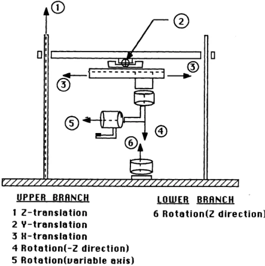
In an attempt to model the kinematic motion of the scanning machine, the transfor-mation techniques previously described were applied to the two open loop chains of the scanning machine. In the kinematic modelling of the actual scanning machine, the application of quaternion transformations provided an eloquent representation of the kinematic characteristics of the machine. The overall design of the scanner is ex-tremely compatible with this notation. Coaxial and orthogonal axes of motion allow the transformations to be greatly simplified. Figure 3.1 shows the kinematic pairs and their relative orientation in the kinematic chain. The joints were modelled by either a prismatic joint for linear motion or a revolute joint for rotational motion. This bifur-cated setup is arranged with the top branch containing three translational motions in the x, y, and z direction and two rotational motions. The lower branch contains one rotational motion (7]. Table 3.1 illustrates the actual joint design used in the scanner and the corresponding joint model and parameters. It should be noted the transducer rotations are driven by stepper motors with a microstep of 0.05'. All other pairs are driven by stepper motors with an incremental half step, A6, of 0.90. The parameters

n, through n6 correspond to the number of steps for each joint motor. The

transla-tional joint have an additransla-tional parameter that defines the pitch of the translation, p. In all, the scanner is capable of a five degrees-of-freedom because two of the motions

3_ I//// //////// /////,/// UPPER BRANCH

1 Z-translation

2 Y-translation 3 H-translation 4 Rotation(-Z direction) 5 Rotation(variable axis) LOWER BRANCH 6 Rotation(Z direction)

Figure 3.1: Relative orientation of kinematic pairs in the bifurcated scanning applica-tion.

O [ ~

/_0

Table 3.1: Model and parameters for scanner joints

3

Pair

L

Description Model Parameters

1 Ball Screw Prismatic Joint nip11,AE11

2 Lead Screw Prismatic Joint n₂,P_{2 2}, A0 2 2

3 Lead Screw Prismatic Joint n₃,P_{3 3}, A( 33

4 Floating Rotation Revolute Joint n4, A944

5 Floating Rotation Revolute Joint ns, Az5 5

6 Base Rotation Revolute Joint n6, Ae6 6

are redundant.

Applying the quaternion transformation notation directly to the kinematic chain, Figure 3.2 illustrates the values of the parameters &,i and 6, which describe the rela-tive positions between the unit screws S,* representing the axis of the kinematic pairs. Screws S* and S8* correspond to the transducer beam and surface normal vector, respec-tively. The parameters aij and Oe are given in Table 3.2. Using eqns.(2.10),(2.11),(2.12) and (2.13) which define the quaternion transformation, the transformations Qi, and Qi

between sucessive links and sucessive pairs can be determined. Applying screw calculus and simple substitution, the transformations reduce to:

Q12 = QI71 (3.1)

Q23

= -E 23 + Q2Q1 r1 Q34 = Q₃Q₂

Q

₁

a*r

₁ Q4 = 1 + Q4Q3Q2Q1&*1E 45 Q56 = Q5Q4Q3Q2Qarl Q67 = Q6Q5Q4Q3Q2Q71 ₁ Q8N = cOS(a8N) - Ea8Nsin(a8N) + *Nsin(a8N) + Ea8NCOS(a8N)

sg

a* 12 I MPM ...

_CL-f

0 4* , 23 *'i 44 s* _L 45 | * *4 a * 67 6 6 S * 5 JLTRASONI TRANSDUCE S 55 S 66 At a* 34 7

070,S:

a 23 8N R 8 KNEE BONE S ol a* 45 5* I Sagn ten

GROUND

Figure 3.2: Symbolic representation of the kinematic chain of the scanning machine.

Table 3.2: Scanner link and pair parameters Angle Length 12 900 0 23 900 a23 34 900 0 45 00 a_{4 5} 56 900 0 67 900 0 8N a8N a8N

Pair Angle Length

1 00 Sol + niplle 11 2 00 _{n 2}P2 2AE)22 3 00 n₃p33A E33 4 n4AE)4₄ S4 4 5 n₅

LeA

₅₅ S_ 6 n5ae 55 S66 7 00 S77 8 n6AEeo6 0

Q2 = 1 + Q1 2S*E(n2P2 2AE)2 2)

Q3 = 1 + Q23Q12S1 E(n3P33Ae 3 3)

Q4

= cos(n4AG44 ) - ES4 4sin(n4Ae4 4) +

(Q34Q23Q12S)sin(n4 AE 44) + ES4 4cO8(n4AE4 4)

Q

= cos(n5A05 5) - ES5 5sin(n5 AG5 5) +

(Q4sQ34Q23 Q12 *)sin(nsAE)ss) + Es5 5cOs(n5Ae)5 5)

Q6 = cos(n5AO55) - ES6 6sin(n5AE)5 5) +

(Q56Q45Q34 Q23Q 2 5*)sin(n5AE ss) + ES6 6cOs(n5AEs55)

Q 1+ Q67 Q56 Q4 Q34Q23Q12S1

Q8 = cos(n₆Ae66) + $8*sin(n6 A 6er6)

This kinematic model assumes that the normal vector to a surface is known, therefore, the link aN from the base rotation to the surface normal will also be known for the kinematic model. Inserting the numerical values from the scanning machine of the con-stant parameters into the transformations gives the final result for the transformations

(See Table 3.3 for parameter values).

Q12 = Q1a7l (3.3) Q23 = E(1.1) +

Q

₂

Q

₁

47

₁ 34= Q₃Q 2

Q

1a71 45= 1 + 94Q3Q2Q1 *1E(3.25) Q56 = QsQ4Q3Q2Q1 rl Q67 = Q6Q5Q4Q3Q2Q1* 1

Q8N = cos(a8N) - Ea8Nsin(a8N) +0 ₈Nsin{a8N) + Ea8NcoS(a8N)

Table 3.3: Values of the critical scanning machine dimensions Dimension Value 012 900 a12 0 a23 900 a23 1.1 in. C934 900 a34 0 a45 00 a45 3.25 in. f56 900 a56 0 067 900 a67 0 a8N 900 a8N 0 So1 2.66 in. S4 4 2.93 in. S55 3.00 in. See 3.15 in. S77 1.80 in. ______ 0.9 /step

Microstep AE9i 0.050/step

p11 18 threads/in.

P22 40 threads/in.

Q3 = 1 + Q23Q12 S*E(n3(.63 * 10-4)

Q4 = cos(n4(.05)) - E(2.93)sin(n4(.05)) +

(Q3 4Q23Qi12 *)sin(n4(.05)) + E(2.93)cos(n4(.05))

Q5 = cos(n5 (.05)) - E(3.00)sin(ns (.05)) + (Q4 5Q34Q23 912 &*)sin(ns (.05)) + E(3.00)cos(ns (.05)) Q6 = cos(n5(.05)) - E(3.15)sin(n5(.05)) + (Q5 6Q4 5Q34 Q2 3Q21*)sin(ns (.05)) + e(3.15)cos(ns(.05)) Q7 = 1 + Q6 7Q5 6Q4 5Q3 4Q23Q12S Q8 = cos(ne(1.8)) + $8*sin(n(.9))

Keeping in mind that the intent of all this notation is to locate the transducer beam and the surface normal line in space, these positions can be represented by combining the transformations that were just developed. The transducer position S. is given by combining subsequent transformations along the manipulator chain:

7 = (Q67Qs6Q4sQ34Q23Q12) * (3.5)

Whereas the normal line position in space SA is given by:

*= (Q8N)S8 (3.6)

The alignment of the two lines is therefore just a matter of equating the two lines. The kinematic model for this bifurcated system is:

Chapter 4

Trajectory Planning Algorithm

Eqn.(3.5) is a set of twelve equations (six real and six dual equations) that define all the solutions that will align the transducer beam with the surface normal vector. However, there are many such solutions that will satisfy the equation. By constraining the problem, a feasible set of solutions can be determined. Speed, accuracy, and obstacle avoidance are constraints that will have to be incorporated in the trajectory planning. These will not be discussed as they are beyond the scope of this thesis. Instead the constraint will be to follow a straight line trajectory path which will provide the fastest movement of the transducer beam. This can be accomplished by driving the transducer beam and surface normal vector into a coplanar orientation where the two lines can be driven together along the plane. By driving the lines along the plane, the alignment of the lines will be accomplished by a final rotation of the transducer within the plane.

The coplanar constraint can easily be expressed as the dot product of the vectors that define the transducer and normal position. Given that the vectors are represented by transformations, the coplanar condition is satisfied if the the dot product of the transformations are equal to zero 13].

QT - QN = 0 -+ coplanar (4.1)

Given the general background for the trajectory planning, the final problem will be to solve the equations. It turns out that the kinematic model produces twelve nonlinear

transcendental equations for the set of values that will align the transducer and surface normal. The constraint imposed produces two nonlinear transcendental equations.

Two methods were used to solve the problem. First, a mathematical computer package called Mathematica

[17]

was used to aid in both the quaternion multiplication necessary to develop the transformations, and in finding a closed form solution of the equations of motion. Second, an iterative computer program was developed to solve the nonlinear constrained programming problem.

4.1

Mathematica

Mathematica is a computer package designed for doing numerical and symbolic cal-culations, and programming in an extremely interactive way. For the application to dual quaternion transformations, Mathematica aided in the development of the trans-formations by performing the complicated dual quaternion multiplications. This was accomplished by using a function that would perform the quaternion multiplication defined in eqn.(2.9). This function can be seen in Figure 4.1. This function f[} takes the inputs a to h, which correspond to the real numbers of the dual quaternion defined in eqn.(2.8). The function performs the cross product(vc) and dot product(vd) of the vector components, the multiplication of the scalar and vector components(slv2,s2vl),

and the multiplication of the two scalar components(sls2). This package proved use-ful to develop the transformations, however, Mathematica was unable to handle the dual part notation of the dual quaternion effectively. Therefore, the word 'dual' was used as a symbol in the formula where anything multiplied by it was considered a dual part. The output was harder to interpret because of the use of this symbolic nota-tion. Despite the confusing notation, the function worked extremely well when called to multiply complicated quaternions.

Mathematica was used to produce the final equations of the kinematic model that represent the solution for alignment of the two branches of the kinematic chain. It was

f/: f[a , ao , b , bo , c , Co , d , do , e , eo , f , o , g, go , h_, ho T

Vc~b, bo, c, co, d, do, f, fo, g, go, h, ho]

-vd[b, bo, c, co, d, do, f, fo, g, go, h, ho] +

slv2[a, ao, f, fo, g, go, h, ho] +

s2vl[e, eo, b, bo, c, co, d, do] + sia, ao, e, eo]

vc/: vc(b , bo , c , co , d , do , f ,

fo

, g , go , h , ho

I

:=

(c*h -g*d + duil*(Eo*h + c*lio - go*d~- g*ao))*i + ~

(b*h - f*d + dual*(bo*h + b*ho - fo*d - f*do))*j +

(b*g - f*c + dual*(bo*g + b*go - fo*c - f*co))*k

vd/: vd[b , bo , C, co , d , do , f , fo , g , go_, h , ho ]

b*f~+ c*g + 3*h +~duaT*(bo~f +~b*fo+ co*g + c*go + dE*h + d*ho)

slv2/: s1v2[a , ao , f , fo , g , go , h , ho]

:-(a*f + duaT*(a&*f +~a*fo))*i + (a*g + dual*(ao*g + a*go))*j +

(a*h + dual*(ao*h + a*ho))*k

s2vl/: s2vl[e , eo , b , bo , c , co , d , do ]

(e*b + duaT*(e3*b +~e*b3))*i~+ (e*c + dual*(eo*c + e*co))*j + (e*d + dual*(eo*d + e*do))*k

s/: s[a_ , ao_, e_, eo_] := a*e + dual*(ao*e + a*eo)

believed .at Mathematica would also be able to give a closed form solution of the equations. It was hoped that the required steps of each stepper motor needed to align the transducer beam and normal line could be determined. Mathematica was unable to handle the complicated equations that were developed from the kinematic model. Adding to the problem was the fact that the equations contained transcendentals.

4.2

Iterative Programming Method

The problem was set up as a nonlinear constrained programming problem with the constraint equations acting as the cost function and the kinematic model equations, which were determined by Mathematica, defining the general set of feasible solutions for the movement of the scanner. An iterative program was used to attempt to solve the nonlinear programming problem for a move from point A to point B. In the trajectory control algorithm, this calculation would be performed for each sucessive step of the scanner.

A program which solves a general nonlinear programming problem using a succesive quadratic programming algorithm and a finite difference gradient was taken from the IMSL Fortran Math/Library, and used to solve the trajectory problem. This function requires a user supplied subroutine that calculates the value of the equations at a given point. Although the general program was set up, a solution for the equations was not obtained.

Chapter 5

Conclusion

A kinematic model describing the motion of an ultrasound scanning machine with a bifurcated manipulator setup was developed. Various representations including point transformations, matrix line transformations and dual quaternion transformations based on screw representation were investigated to detemine their efficiency and applicabil-ity to kinematic modelling of open loop chains. Screw representation was shown to be the most general way to represent the motion of rigid bodies, thus providing more information about the motion and orientation of the links in a manipulator chain. In the case of the ultrasound scanning machine, the transformation of screws was highly applicable because of the need to align lines in space rather than position points.

A study of the efficiency of the various transformations showed that the dual quater-nion transformations provided the most efficient and eloquent representation of the relative motion and orientation of the links and joints in the kinematic system. Dual quaternions provide the minimal number of parameters needed to define the transfor-mation between two lines in space, while at the same time, require less computational effort. Traditional matrix transformation require 216 multiplies whereas dual quater-nions require only 96 multiplies.

Therefore, using the dual quaternion approach and dual vectors, the kinematic model for the scanner was developed. Two techniques were used to solve the system of

equations that describe the trajectory of the scanner. First, Mathematica, a computer package for doing mathematics was used to perform the dual quaternion multiplications and to determine the closed form solution of the system of nonlinear equations. The computer package could do the quaternion multiplication fairly well, however, it was unable to determine the closed form solution. Second, an iterative program was written utilizing the IMSL Fortran Math/Library to solve the nonlinear programming problem for a movement from one point to another, given the constraint that the optimum trajectory should be along a straight line path. This was accomplished by using a constraint that would position the transducer beam and normal vector in a plane so that they could be driven together along that plane. A solution could not be obtained in the time available.

Overall, it has been shown that dual quaternion transformations and screw repre-sentation are efficient and compact ways to represent an open loop kinematic chain. The technique has been applied to the ultrasound scanner producing a kinematic model for the motion and orientation of the transducer and normal vectors.

Although the techniques decribed are extremely helpful in developing the kinematic model of the scanning machine, more time and effort needs to be directed toward incorporating the other constraints of speed, accuracy and obstacle avoidance into the kinematic model of the scanning machine. Also, an effective method to optimally solve the equations should be developed. The trajectory control of this scanner is extremely complicated and will require more research to produce an efficient scanning algorithm given the numerous constraints.

Bibliography

[1] Ateshian, G.A. Stereophotogrammetric determination of patellar cartilage thick-ness and surface geometry. In G.R. Miller, editor, 1988 Advances in

Bioengineer-ing, pages 164-174, November 1988.

[2] Ball, R.S. A Treatise on the Theory of Screws. Cambridge University Press, Cambridge, 1900.

[3] Brand, L.S. Vector and Tensor Analysis. John Wiley and Sons, New York, 1947. [4] Clifford, M.A. Preliminary sketch of biquaternions. Proc. of the London Math.

Soc., 4:381-395, June 1873.

[5] Hamilton, W.R. Elements of Quaternions. Longmans, Green, and Co., London, 1899.

[6] Hunt, K.H. Kinematic Geometry of Mechanisms. Clarendon Press, Oxford, 1978. [7] Ito, K. An Ultrasonic Transducer Positioner. BS thesis, Massachusetts Institute

of Technology, Cambridge, 1985.

[8] Langrana, N.A., Leppard, D., Alexander, H. and Weiss, A. Kinematics of the knee

- A computer graphics model. Technical Report 82-DET-40, ASME, 1982.

[9] Paul, R.P. Robot Manipulators: Mathematics, Programming and Control. MIT Press, Cambridge, MA, 1982.

[101 Rooney, J. A comparison of representations of general spatial screw motion.

En-vironment and Planning B, 5:45-88, 1978.

[111 Roth, Bernard. Screws, motors, and wrenches that cannot be bought in a hardware store. Robotics Research, 1:679-693, 1984.

[12] Rushfeldt, P.D. Human Hip Joint Geometry and the Resulting Pressure

Distribu-tion. PhD thesis, Massachusetts Institute of Technology, Cambridge, 1978.

[13] Seering, W.P. Robotics and manufacturing-a perspective. Robotics Research,

1:973-982, 1984.

[14] Sheth, P.N. and Uicker, J.J. Jr. A generalized symbolic notation for mechanisms.

J. Eng. for Ind., Trans. ASME Series B, 93:102-112, 1971.

[15] Sugimoto, K. and Matsumoto, Y. Kinematic analysis of manipulators by means of the projective transformation of screw coordinates. Robotics Research, 1:695-705,

1984.

[16] Walker, P.S., Rovick, J.S., and Robertson, D.D. The effects of knee brace hinge design and placement on joint mechanics. J. Biomechanics, 21(11):965-974, 1988. [171 Wolfram, S. Mathematica. Addison-Wesley Publishing Co., New York, 1988. (181 Yang, A.T. Application of Quaternion Algebra and Dual Numbers to the Analysis

of Spatial Mechanisms. PhD thesis, Columbia University, New York, 1963.

[19) Yuan, M.S.C. and Freudenstein, F. Kinematic analysis of spatial mechanisms by means of screw coordinates. Part I - Screw coordinates. J. Eng. for Ind., Trans.

ASME Series B, 93:61-66, February 1971.

[201 Yuan, M.S.C., Freudenstein, F. and Woo, L.S. Kinematic analysis of spatial mech-anisms by means of screw coordinates. Part II - Analysis of spatial mechanisms.