DEPENDABILITY MODELING AND EVALUATION OF SOFTWARE-FAULT TOLERANT SYSTEMS

HAL Id: hal-01978863

https://hal.laas.fr/hal-01978863

HAL is a multi-disciplinary open access archive for the deposit and dissemination of sci-entific research documents, whether they are pub-lished or not. The documents may come from teaching and research institutions in France or abroad, or from public or private research centers.

L’archive ouverte pluridisciplinaire HAL, est destinée au dépôt et à la diffusion de documents scientifiques de niveau recherche, publiés ou non, émanant des établissements d’enseignement et de recherche français ou étrangers, des laboratoires publics ou privés.

Jean Arlat, Karama Kanoun, Jean-Claude Laprie

To cite this version:

Jean Arlat, Karama Kanoun, Jean-Claude Laprie. DEPENDABILITY MODELING AND EVALUA-TION OF SOFTWARE-FAULT TOLERANT SYSTEMS. IEEE Transactions on Computers. Special Issue on Fault-Tolerant Computing, 1990, 39, pp.504 - 513. �hal-01978863�

DEPENDABILITY MODELING AND EVALUATION OF SOFTWARE-FAULT TOLERANT SYSTEMS1

JEAN ARLAT, KARAMA KANOUNAND JEAN-CLAUDE LAPRIE

LABORATOIRED'AUTOMATIQUEETD'ANALYSEDES SYSTÈMESDU C.N.R.S. 7, AVENUEDU COLONEL ROCHE, 31077 TOULOUSE CEDEX - FRANCE

ABSTRACT

The paper provides dependability modeling and evaluation (encompassing reliability and safety issues) of the two major fault-tolerance software approaches: recovery blocks (RB) and N-version programming (NVP). The study is based on the detailed analysis of software fault-tolerance architectures able to tolerate a single fault (RB: two alternates and an acceptance test, NVP: three versions and a decider).

Keywords: Software Design Diversity, Software Fault Tolerance, Dependability Modeling, Dependability Evaluation.

INTRODUCTION

A number of papers devoted to the dependability analysis of software fault-tolerance approaches have appeared in the literature, for which two major goals can be identified: (i) modeling and evaluation of the dependability measures [7, 13, 14 ,17, 23, 27, 28], (ii) detailed analysis of the dependencies in diversified software [6, 10, 21, 26].

This paper is an elaboration on the work presented in [2] and belongs to the first

1 _{This reseach has been carried out in the framework of the Hermès European Space Shuttle Project and of the ESPRIT project}

[8]. The major extensions to published work concern: (i) the definition of a unified modeling framework based on the identification of the possible types of faults through the analysis of the software production process [17], (ii) the evaluation of both reliability and safety measures and (iii) the consideration of two specific characteristics of the architectures that have received little treatment up to now: the discarding of a failed version, for NVP, and the nesting of the blocks, for RB.

Two classes of faults are considered: independent faults and related faults [3]. Related faults result either from a fault in the common specification, or from dependencies in the separate designs and implementations. Two types of related faults may be distinguished: (i) among several variants (alternates for RB or versions for NVP) and (ii) among one or several variants and the decider (the acceptance test of the RB or the voting algorithm of NVP). Related faults manifest under the form of similar errors, whereas we shall assume that independent faults cause distinct errors2* .

Since the faults considered are design faults that are introduced in the software, either during its specification or during its implementation, we shall start the analysis of each approach by relating the various types of faults to the production process [17].

When a failure occurs, the detection of the inability to deliver acceptable results may be an important consideration, in that sense that an undetected failure may have, and generally has, catastrophic consequences. Although the notion of safety strongly depends on the considered application, in practice, the

2 * Although they could be traced to independent faults, faults leading to similar errors are not distinguishable at the execution level from related faults and thus they will be merged into the category of related faults.

detection of the inability to deliver proper service is a prerequisite to initiate the specific safety procedures. A detected failure (no acceptable result is identified by the decider and no output result is delivered) will thus be termed as a benign failure, whereas an undetected failure (an erroneous result is delivered) will be termed as a catastrophic failure.

As usual, we shall consider reliability as a measure of the time to failure and safety as a measure of the time to catastrophic failure.

Software faults can manifest only when it is executed. We shall thus consider the execution process and the fault manifestation process.

The general behavior model is given in figure 1. Transition from B to I stands only for safety, in which case it is assumed that it is possible to restore service delivery by means of procedures carried out at an upper level, i.e. supplying input data different from those having led to benign failure. State class C is absorbing for safety whereas both state classes B and C are absorbing for reliability.

End of

Execution

Restoration

of service

Catastrophic Failure

Start of

Execution

Software failed B

Benign Failure

Software under Execution

Software failed C

Idle Software

I

Figure 1: General Behavior Model

We shall assume that the behavior of the systems under consideration can be modeled as a Markov chain; for a discussion of this assumption, see e.g. [9, 17, 20]. The execution process will be modeled through execution rates and the

various components of the software: the variants and the decider. The transition rates outputting from the non-absorbing states are of the form:

λ_{ij = pij . λi with ∑j pij = 1} (1)

where, i designates a non absorbing state, λi is the rate associated to the tasks executed in state i and pij represents the probability of the transition from state i to state j of the model.

When the non-absorbing states (non-failed states for reliability, non-failed and benign failure states for safety) constitute an irreducible set [11] (i.e., the graph associated to the non-absorbing states is strongly connected), it is shown in [24] that the absorption process is asymptotically a Homogeneous Poisson Process (HPP), whose failure rate Γ is given by:

∏ (transition rates of the considered path )

Γ = ∑ _____________________________________________________ (2) paths from ∏ { ∑ (output rates of the considered state) }

initial state (I) to states in absorbing state (s) path

(I excepted)

The rate of convergence of the absorption process towards the asymptotic HPP is directly related to the execution rates; it is thus reached very rapidly (say, after three executions). We shall adopt this approach in the following whenever possible, and we shall denote as equivalent rate, the rate of the asymptotic HPP. ΓR will denote the equivalent failure rate for reliability and ΓS is the equivalent catastrophic failure rate for safety.

Using relations (1) and (2), it can be easily verified that the equivalent failure rates can be expressed simply using: (i) the departure rate σ from state I of figure 1 and (ii) the probability of failure of the software obtained from the embedded discrete chain. Let QR (resp. QS) be the probability of failure (resp.

catastrophic failure), thus:

Γ_{R = σ QR,} Γ_{S = σ QS} (3)

Accordingly, reliability (R(t)) and safety (S(t)) are given by:

R(t) = exp (-ΓR t) S(t) = exp (-ΓS t) (4)

As QR and QS are evaluated directly from the discrete Markov chain, in the sequel we focus essentially in the presentation of the discrete Markov chains describing the fault manifestation process of the fault-tolerant softwares.

Finally, it is worth noting that we focus on the fault-tolerant software itself, i.e. the underlying mechanisms are not considered: (i) recovery point establishment and restoration for RB, and (ii) synchronisation of the versions, cross-check points establishment for NVP.

The sequel of the paper is organized into four sections. Sections 1 and 2 present respectively the analyses of RB and NVP: for each approach a detailed model based on the production process of the fault tolerant software is first established and then it is simplified through the assumptions that only a single fault type may manifest during execution of the fault tolerant software and that no error compensation may take place within the software. Section 3 introduces some elements for RB and NVP comparison. Section 4 analyzes the nested RBs.

1. RECOVERY BLOCKS

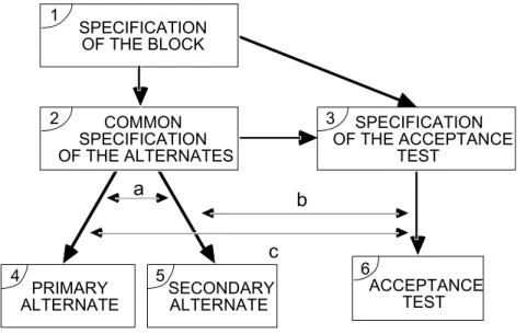
Figure 2-a shows the production process of a RB with two alternates (a primary (P) and a secondary (S)), and one acceptance test (AT). During the diversified designs and implementations of P & S and of AT, independent faults may be created. However, due to dependencies, some related faults between P and S or between P & S and the AT may be introduced. Faults committed during common specification (path 1 → 2, 1 → 3 , 1 → 2 → 3) are likely to be related faults and, as such, the cause of similar errors. Faults created during the implementation can also lead to related faults between P & S and AT (channels a, b, c); all these faults are summarized in figure 2-b. It is worth noting that the probabilities listed could be obtained from controlled experiments such as the one reported in [1].

For deriving the fault manifestation model, a question immediately arises: what types of faults are considered as possibly manifesting as the consequence of their activation? This leads to consider successively the following assumptions:

A1: only a single fault type (either independent or related) may manifest during the execution of an alternate and the AT and no error compensation may take place within an alternate and the AT during an execution, i.e. an error is either detected and processed or leads to catastrophic failure. A2: only a single fault type may manifest during the execution of the whole RB and no error

compensation may take place within the RB.

The detailed model will be based on assumption A1, which enables some singular behaviors of the decider to be characterized.

SPECIFICATION OF THE BLOCK 1 COMMON SPECIFICATION OF THE ALTERNATES 2 _{SPECIFICATION} OF THE ACCEPTANCE TEST 3 PRIMARY ALTERNATE 4 SECONDARY ALTERNATE 5

a

b

c

a) Fault Sources in RB Production Process

Path where Fault (s) Probability is (are) Created Fault Type (s) of or Dependency Channel (s) Activation

1 → 2 or (a) Related fault in P and S _qPS

1 → 3, (c) or 1 → 2 → 3 Related fault in P and AT (or P, S and AT) _qPT*

(b) Related fault in S and AT _qST

2 → 4 or 2 → 5 Independent fault in P or S _{qP or qS}

3 → 6 Independent fault in AT _qT

* Since the activation of a related fault between P and AT leads to RB failure, no further decomposition with respect to the faults of S is necessary.

b) Fault Types and Notation for RB Figure 2

1.1. Detailed RB Model

Figure 3 describes the M1 model based on the notation of figure 2-b. P, TP, S and TS form the Software under Execution class from figure 1, respectively: execution of P, execution of AT after P, execution of S, execution of AT after S.

q

q

p'

q

p

q

q

C

1

p

q

q'

1

1

q"

q'

1

1

p

p"

p'

TP4

TP3

S1

S3

TS1

TS4

TP1

TS2

TP2

S2

B

1

1

TS3

q'

1

I

P

Figure 3: M1 - Detailed RB Model

Different states are considered for TP to account for the various types of faults that may be activated in P:

TP1) no fault activated [pP],

TP2) activation of an independent fault [qP],

TP3) activation of a related fault between P and S [qPS], TP4) activation of a related fault between P and the AT [qPT].

This partition leads to a subsequent decomposition of states S and TS. It is assumed that no fault can be activated in AT after activation of an independent fault in P (unity transition from state TP2): these faults are considered as consisting essentially of related faults and, as such, are accounted for in

probability qPT leading to state TP4. Activation of a related fault between P and S (state TP3) corresponds to a detected failure and leads through S3 and TS3 to state B. The activation of a related fault between P and AT (state TP4) corresponds to a catastrophic failure and leads to state C.

Due to the fact that S is executed only when an independent fault has been activated either in P or in AT, conditional probabilities have been introduced in the model; in particular:

qS = Prob { activation of an independent fault in S | S is executed after activation of a fault in P } q'S = Prob { activation of an independent fault in S | S is executed after activation of a fault in AT } The same differences in the conditions apply for qST and q'ST and also for the probabilities of activation of an independent fault in the AT following the execution of S: q'T and q"T .

The path π = {P, TP1, S1, TS1, I} corresponds to an error compensation identifying a singular behavior of the AT: the AT rejects an acceptable result provided by P and subsequently accepts the result given by S.

It is worth noting that M1 can be reduced when considering that:

- qT ≈ q'T , qS ≈ q'S , qST ≈ q'ST: the probabilities of activation of a fault in S (or AT) following the activation of an independent fault either in P or in AT are equivalent, since in any case their execution is a consequence of the application of error-prone input data,

- p"T << 1: error compensation (path π) is unlikely to occur,

- each state belonging to the Software under Execution class with an outgoing transition equal to 1 can be merged with the next state,

q_T p_T P I TS2 S1 C B p_T q_P p_P q_PS q_PT p_S q_ST q_ST 1 - qST q_T q_S TP2 TP1 p_T 1 Figure 4: Model M'1 1.2. Simplified RB Model

In this case, since assumption A2 applies, a single fault type can be activated in the whole RB; thus transitions from S1 and S2 to TS4 of model M1 (resp. S1 to C for M'1) must be deleted. This is equivalent to make qST = 0 and to merge the related faults between S and AT with the related faults between P and AT; it follows that qPT becomes qPST. The corresponding model (M2) is given in figure 5.

1.3. Processing of the Models

Assuming that pP ≈ 1-qP and pS ≈ 1-qS, we obtain for models M1 and M'1: for reliability: ΓR = σ { qPS + qPT + qT + qP [qST + qS (1 - qT)] }(5)

for safety: ΓS = σ { qT qST+ qPT + qP qST (1 - qT) } (6)

For model M2, we obtain:

Γ_{R = σ { qPS + qPST + qT + qP qS (1 - qT) }} (7)

P

q

q

q

C

I

1

B

p

q

q

T

S

p

1

p

Figure 5: M2 - Simplified RB Model 1.4. Comparison with a Non Fault-Tolerant Software

The comparison with a non fault-tolerant software leads to consider a software with no internal fault detection mechanism whose failure rate is equal to the sum of the elementary failure rates of an alternate:

Γ'_{R = σ { qP + qPS + qPT }} (9)

where qPT must be replaced by qPST when considering assumptio A2.

Comparison is presented for reliability only, since the notion of safety as defined here does not apply to a software with no internal detection mechanisms. Let define r as: r = ΓR / Γ'R; the RB provides a reliability improvement if r < 1. This leads to:

For model M'1: _{qT < qP (1 - qP - qST) / (1 - qP qS)} (10)

For model M2: qT < qP (1 - qS) /(1 - qP qS) (11)

Since the AT is usually less complex than P or S and assuming that complexity and probability of failure are related, we have qT << qP, which enables relations (10) and (11) to be verified. However, the quantification of the improvement must be studied for each specific case.

2. N-VERSION PROGRAMMING

The potential sources of faults in the production process of a NVP software with three versions and one decider are shown on figure 5-a.

As the versions correspond to operational software of good quality, it can be assumed that they are of equivalent reliability, and thus:

A3: The probability of fault activation is the same for the three versions3*.

This leads to the following notation:

qIV = Prob { activation of an independent fault in one version } q2V = Prob { activation of a related fault between 2 specific versions } q3V = Prob { activation of a related fault between the 3 versions }

Two other probabilities are defined in order to account for the faults of the decider: qD = Prob { activation of an independent fault in the decider }

qVD = Prob { activation of a related fault between the 3 versions and the decider}

The probabilities concerning the versions could be evaluated from controlled experiments such as [1, 15]. However, these experiments do not account for the analysis of the faults in the decider. The presented models and decider-associated probabilities enables the performance of various voters under failure conditions shuch as the ones theoretically investigated in [22] to be accounted for and may constitute a framework for conducting more comprehensive and more adapted experiments.

Figure 6-b summarizes this notation and relates the considered types of faults with the production process of figure 6-a.

3 * This assumption is used only to simplify the notation and do not alter the significance of the results obtained; the generalization to the case where the characteristics of the versions are distinguished can be easily deduced.

SPEC. OF

THE NVP

1

COMMON SPEC.

OF THE VERSIONS

2

_{SPEC. OF}

THE DECIDER

3

DECIDER

7

d

V # 2

5

a

c

V # 3

6

V # 1

4

b

a) Fault Sources in NVP Production Process.

Paths where faults Fault types Probability

are created or of activation

dependency channels

1 → 2 Related fault in the 3 versions _q3V

(a), (b) or (c) Related fault in 2 versions _q2V

1→2→ 3, 1→3 or (d) Related fault in versions and decider _qVD

2→4, 2→5 or 2→6 Independent fault in a version, _qIV

3 → 7 Independent fault in the decider _qD

b) Major Fault Types and Notation for NVP Figure 6

Further notation will be introduced when required; in particular, let qV denote the probability of activation of a fault in any version, thus from assumption A3 we have:

qV = q3V + 2 q2V + qVD + qIV (12)

An important characteristic to account for is related to the fact that besides error processing procedures (majority vote based on cross-checks [8], selection of the median result [4] or other voters identified in [22], etc.), the decider

Accordingly, the following assumptions will be considered successively:

A4: No fault treatment is carried out after error processing: should a version disagree with the result selected by the decider, the version is kept in the NVP architecture and supplied with the new input data4*.

A5: Fault treatment is carried out: it consists in the identification of a disagreeing version and its elimination from the NVP architecture.

2.1. NVP Model Without Fault Treatment

In this case, the major specification of the decision algorithm is only to provide an acceptable output result when the versions provide at least two acceptable results.

Due to the fact that, (i) the versions are executed in parallel and (ii) the decision of acceptance of the current execution and selection of the "best" result is made on a relative basis, the dependability analysis of NVP requires that the interactions between the faults in the versions and the faults in the decider, as well as their consequences, be precisely identified. Thus, as for RB, we consider the following assumptions:

A6: Only a single fault type may manifest during the execution of the versions.

A7: Only a single fault type may manifest during the whole NVP software execution (versions and decider) and no compensation may take place between the errors of the versions and of the decider.

4 * This applies when faults exhibit a soft behavior [10, 17], i.e. when it is likely that the fault will not recur in next execution.

2.1.1. Detailed NVP Model

The behavior of NVP when considering assumption A6 is described by model M3 shown in figure 7.

B _C p IV 3 (q )2 q D1B q D1C q D4A q D5B 1 1 3 q 2V p _D1A D2 q 3V IV 3 q D3 D4 D1 p D5C D5 q D5A q D3A V p D2A I p D3B q D4B q D2Cq D3C p D4C q _D2B

p = 1 - 3 qIV - 3 (qIV)2 - 3 q2V - q3V pDiA = 1 - qDiB - qDiC, i = 1,.2

pD3B = 1 - qD3C - qD3A, pDiC = 1 - qDiA - qDiB, i = 4,.5

Figure 7: M3 - Detailed NVP Model Without Fault Treatment

State V is the state when the versions are executed. States Di, correspond to the execution of the decider. Based on A3 and on the impact of the evaluation of acceptable, distinct or similar erroneous results on dependability, five cases are distinguished:

D1: no fault activation[p]; the versions provide 3 acceptable results,

D2: _{activation of an independent fault in 1 version [3 qIV (1 - qV)2 ≈ 3 qIV]; the versions provide 2} acceptable results,

D3: _{activation of independent faults in 2 or 3 versions [3 (qIV)2 (1 - qV) + (qIV)3 ≈ 3 (qIV)2]; the} versions give 3 distinct results,

D5: _{activation of related faults in the 3 versions [q3V]; the versions provide 3 similar erroneous} results.

From these states, the nominal (fault free) behavior [pDiA] resulting from the execution of the decider, leads to a transition from:

- D1 & D2 to I, since the decider evaluates 3 or 2 acceptable results, - D3 to B, since the decider evaluates 3 distinct results,

- D4 & D5 to C: the decider evaluates 2 or 3 similar erroneous results. Considering decider faults, leads to the following singular events:

- error compensation, the decider delivers an acceptable result when evaluating, at least two distinct results (state D3)5*, two (state D4) or three (state D5) similar erroneous results, which leads

to state I; the associated probabilities are denoted qDiA,

- rejection of an execution although at least two similar results are provided by the versions (states D1, D2, D4 and D5)6†, which leads to state B; the associated probabilities are denoted qDiB,

- delivery of an erroneous output result when evaluating, either at least two acceptable, or at least two distinct erroneous results; (states D1, D2, D4 and D5)‡7 leading to state C, the associated

probabilities are denoted qDiC.

As the decision made by the decider is essentially relative, its efficiency depends rather on the similar/distinct than on the acceptable/erroneous aspects of the results to be evaluated; thus, the following assumptions can be considered in practice to simplify model M3:

5 * _{This would take place, for example, in the case of a median-based decision when the erroneous}

results are placed on each side of the acceptable result.

6 † _{The decider is too "tight"; this results in a reliability penalty, in the case when the similar}

results correspond to acceptable results.

7 ‡ _{This case does not correspond to the usual case when the decider is evaluating at least two}

similar erroneous results. The singularities correspond here to the cases — hopefully rare! — when the decider outvotes acceptable results or when the decider is too "loose".

A8: The decider is not able to discriminate similar acceptable results from similar erroneous results, thus: qD1B ≈ qD5B and qD2B ≈ qD4B.

A9: The decider has the same nominal behavior (it provides a common output result) when evaluating either 2 (majority) or 3 similar results; accordingly:

pD1A ≈ pD2A, qD1B ≈ qD2B, and thus qD1C ≈ qD2C, pD4A ≈ pD5A, qD4B ≈ qD5B, and thus qD4C ≈ qD5C. 2.1.2. Simplified NVP Model

The corresponding model (M4) can be directly derived from the analysis of the NVP production process (figure 5-a) and is shown on figure 8.

States D1, D2 and D3 are equivalent to related states of M3. State D4/5' corresponds to the activation of related faults either a) among the versions (merging of states D4 and D5 from M3 [qRV = 3 q2V + q3V]), or b) between the 3 versions and the decider [qVD] (figure 6).

In this case, qVD includes all the interactions between the faults of the versions and of the decider and thus, the impact of the activation of an independent fault in the decider is considered only for state D1 with probability qD = qD1B + qD1C. For states D2, D3 and D4/5', the description is limited to the nominal (fault free) behavior of the decider.

I V D3 D4/5' B 1 p' 3 qIV 3 (q )IV 2 p D1A q _D1B 1 1 1 ₁ D2 q _D1C D1 C q RV+ q VD

p' = 1 - 3 qIV - 3 qIV2 - qRV - qVD pD1A = 1 - qD1B - qD1C Figure 8: M4 - Simplified NVP Model Without Fault Treatment. 2.1.3. Processing of the Models

For model M3:

Γ_{R = σ { (p + 3 qIV) (qD1B + qD1C)}

+ qRV (pD4C+ qD1B)+ 3 (qIV)2 (pD3B + qD3C) } (13) ΓS = σ { (p + 3 qIV) qD1C + qRV pD4C + 3 (qIV)2 qD3C }(14)

For model M4, we have:

Γ_{R = σ { p' qD + qRV + qVD + 3 (qIV)}2 } (15)

Γ_{S = σ { p' qD1C + qRV + qVD }} (16)

for which the expressions below are close pessimistic approximations:

Γ_{R = σ { qD + qRV + qVD + 3 (qIV)}2 } (15')

Γ_{S = σ { qD1C + qRV + qVD }} (16')

It is worth noting that the same expressions can be obtained from M3, (i) when there is no compensation [qD3A = qD4A = 0] and (ii) noting that expression [3 qIV qD1C + 3 (qIV)2 qD3C] obtained in (13) and (14) can be identified to the probability of activation of a related fault in the versions and in the decider [qVD] from (15) and (16). Indeed, (13) and (14) write as:

Γ_{R = σ { (p + 3 qIV + qRV) qD1B + p qD1C + qRV pD4C + qVD}

Γ_{S = σ { p qD1C + qRV pD3C + qVD }} (14')

for which it can be verified that (15') and (16') constitute valid approximations. Accordingly, further analyses will be carried out considering essentially these approximate expressions.

2.1.4. Comparison with a Non Fault-Tolerant Software

From (12) the failure rate of the non fault-tolerant software corresponding to the selection of any version is expressed as:

Γ'_{R = σ qV = σ {q3V + 2 q2V + qVD + qIV} = σ {q'RV + qVD + qIV}} (17)

where q'RV corresponds to the probability of activation of the faults in the selected version that could be mapped to related faults in the other two versions in the NVP software. The ratio r = ΓR / Γ'R is then:

r = \F(qD + qRV + qVD + 3 (qIV)2;q'RV + qVD + qIV) (18)

For the comparison, we introduce the ratio i identifying the proportion of independent faults in the selected version:

qIV = i qV = i (q'RV + qVD + qIV) (19)

It follows that:

r = \F(qD;qV) + \F(qRV + qVD;qV) + 3 (i)2 qV (20)

As qRV = q3V + 3 q2V and q'RV = q3V + 2 q2V, we have qRV ≈ q'RV, when related faults in 3 versions dominate (specification), and qRV ≈ (3/2) q'RV, when related faults in 2 versions dominate (implementations). Thus, r is comprised into domain determined by the lower (r') and upper (r") bounds:

r' = qD/qV + (1 - i) + 3 (i)2 qV (21)

r" = qD/qV + (3/2) (1 - i) + 3 (i)2 qV (22)

- if related faults dominate (i ≈ 0) no improvement has to be expected, which confirms the results obtained in a large number of previous studies, e.g. see [16, 21],

2.2. NVP Model With Fault Treatment

In this case (since assumption A5 applies), a supplementary specification of the decider is to correctly diagnose a disagreeing version when two versions provide acceptable results.

2.2.1. Description of the Model

The corresponding model (M5) is shown on figure 9.

p'

1

1

B*

C*

D*

p*

q* + q*

p*

q*

q*

1

2 q

+ (q )

I

+

q

q'

V

B

C

3 (q )

3 q

p"

q'

q'

1

D

I*

V*

Submodel SM1 is equivalent to model M4, the only differences concern:

- the elimination of the states Di with an output transition equal to 1 by merging them with the next state,

- the modification of the probabilities of activation of a fault in the decider to account for the change in its specification, (i) change of qVD into q'VD8* and (ii) change of qD1i into q'Di (i ∈ {B,C}),

- when an independent fault has been activated in a single version, this version is discarded and thus SM2 is entered.

SM2 has the same structure as SM1; however, as only 2 versions are used, the probabilities of fault activation in the versions and in the decider are modified in accordance; in particular, q*RV = q2V. 2.2.2. Processing of the Model

As in model M5 the non-failed states do not constitute an irreducible Markov chain, it is not possible to obtain equivalent failure rates. However, equivalent failure rates may be derived for each submodel in isolation:

for SM1: Γ_{R1 = σ { q'D + qRV + q'VD + 3 (qIV)}2 } (23)

Γ_{S1 = σ { q'DC + qRV + q'VD }} (24)

for SM2: Γ_{R2 = σ { q*D + q*RV + q*VD + 2 qIV + (qIV)}2 } (25)

Γ_{S2 = σ { q*DC + q*RV + q*VD }} (26)

Reliability and safety of the model can then be analyzed by processing model M6 of figure 10, where X=R for reliability and X=S for safety.

8 * _{In particular q'}

VD includes the risk of failure of the diagnosis of the decider: discarding a version

Γ

Γ

Figure 10: M6 - Model for Reliability and Safety Analysis

Reliability and safety and the associated mean times to failure express as: R(t) = exp [- ( Γ12 + ΓR1) t] + \F(Γ12;Γ12 + ΓR1 - ΓR2) { exp [- ΓR2 t] - exp [- ( Γ12 + ΓR1) t] }

S(t) = exp [- ( Γ12 + ΓS1) t] + \F(Γ12;Γ12 + ΓS1 - ΓS2) { exp [- ΓS2 t] - exp [- ( Γ12 + ΓS1) t] } (27) MTTFR = \F(Γ12;Γ12 + ΓR1) ( \F(1;ΓR2) - \F(1;ΓR1) ) + \F(1;ΓR1)

MTTFS = \F(Γ12;Γ12 + ΓS1) ( \F(1;ΓS2) - \F(1;ΓS1) ) + \F(1;ΓS1) (28)

Analysis of these expressions requires that the rates be precisely evaluated which is a rather difficult task due to the uncertainty in the values of the probabilities from which they are derived. Nevertheless, interesting results can be obtained with the following assumptions:

A10: The decider has the same behavior when evaluating either three versions (SM1) or two versions (SM2), i.e., q'Di ≈ q*Di and q'VD ≈ q*VD,

A11: Due to the intrinsic simplicity of the algorithm involved, the behavior of the decider is not significantly altered when its specifications are modified from assumption A4 (model M4) to assumption A5 (model M5), i.e., qD1i ≈ q'Di and qVD ≈ q'VD.

According to A10, it can be verified from relations (23) to (26), that:

Γ_{R1 = σ { q'D + q3V + 3 q2V + q'VD + 3 (qIV)}2 } (29)

Γ_{S1 = σ { q'DC + q3V + 3 q2V + q'VD }} (30)

Γ_{R2 = σ { q'D + q2V + q'VD + 2 qIV + (qIV)}2 } (31)

These relations show that ΓS1 > ΓS2 and that:

- ΓR1 < ΓR2, when independent faults in the versions dominate, - ΓR1 > ΓR2, when related faults among the versions dominate.

Expressions (28) show that the decision to discard the disagreeing version improves MTTFS, which is not always the case for MTTFR9*. Analogous conclusions can be derived from expressions (27) for S(t) and

R(t).

More generally, the expressions confirm a general system reliability result, i.e. it is better to use two versions than three versions, when emphasis is put on safety rather than on reliability. Furthermore, in the case of reliability, the impact of related faults is clearly indicated by the fact that no improvement has to be expected when using three versions instead of two if related faults among the versions dominate significantly over independent faults [21].

9 * _{Indeed, 1/ΓR1 (resp. 1/ΓS1) can be interpreted as the MTTF}

R (resp. MTTFS) of the NVP software

3. RB AND NVP COMPARISON

In order to be homogeneous, the comparison is carried out only when:

- assumptions A2 and A7 hold (a single fault type activation and no error compensation within the whole software),

- no specific fault treatment is considered for NVP.

For each architecture, specific notations have been used. However, similar expressions can be derived for Γ_{R and ΓS, based on the following notation:}

qI = Prob { independent failure of one variant | execution } thus: qI,RB = qP ≈ qS and qI,NVP = qIV

qCM = Prob { common-mode failure | execution }

thus: qCM,RB = qPST + qPS + qT and qCM,NVP = qVD + qRV + qD Accordingly, relations (7) with qT <<1 and (15') become respectively:

for RB: _{ΓR = σ { qCM,RB + (qI,RB)2 }} (33)

for NVP: ΓR = σ { qCM,NVP + 3 (qI,NVP)2 } (34)

Although the form of these expressions would suggest that RB is better than NVP, it has to be noted that the influence of the various terms may be different. Indeed, if the probabilities of activation of (i) an independent fault in one variant [qP (or qS) and qIV] and (ii) of related faults between variants[qPS and qRV], are of the same order of magnitude, however, the probabilities of activation of (i) an independent fault in the decider [qT and qD] and (ii) of related faults between the variants and the decider [qPST and qVD] are likely to be greater for RB than for NVP; this is mainly due to the fact that the AT is specific to each application, whereas the decider in NVP is generic to a large extent.

It follows that independent failures of the variants have more impact for the NVP, whereas the impact of the decider is lower for this architecture.

However, a precise knowledge of these probabilities would be needed in order to perform a more detailed comparison.

Considering safety analysis, we have obtained:

for RB: Γ_{S= σ qPST} (35)

for NVP: ΓS= σ { qRV + qVD + qD1C } (36)

Related faults among variants have no influence for RB, but are of prime importance for NVP. This is a consequence of the fact that for RB an absolute decision is taken for each alternate against the specification and that for NVP the decision is made on a relative basis among the results provided by the versions.

Due to the very nature of the NVP decider, qD1C may be made very low, thus qVD << qRV and qRV has to be compared with qPST.

Finally it is worth noting that only partial conclusions can be drawn from this analysis. Additional features need to be taken into account, such as the fact that, for RB, service delivery is suspended during error recovery, i.e., when the secondary is invoked.

4. NESTED RECOVERY BLOCKS

This section provides a preliminary extension of the analysis of the RB architecture to account for the specific case of nested RBs. Nested RBs are very interesting and give rise to stimulating discussions, but have received little treatment from the modeling point of view. We simply illustrate here, how a simple case of nested RBs can be handled with the modeling and evaluation approach presented. Let us consider for example that P is itself a RB; P will be called the nested block (NB).

The production process of a RB (figure 2-a) is still the same, but box 4 becomes specification of the NB, and it is decomposed into an equivalent production process as for the original RB (figure 11).

It can be seen that related faults due to the specification still remain; on the contrary related faults introduced, during separate implementations (channels a,b,c) are moved to the lower level, i.e., between the alternates composing the NB and the associated AT, S and the original AT.

Independent faults in S are not changed either, but independent faults in P are split into related and independent faults in the NB.

It follows that the common-mode failure probability (qCM) must be split into Specification and Implementation common-mode failure probabilities denoted (qCMS) and (qCMI), respectively. qCMS is the same for the original and the nested RBs, but the probability of common-mode failure due to implementation faults has to be distinguished for the original (qCMI) and the nested (q*CMI) RB.

SPEC. OF THE NESTED BLOCK 4 COMMON SPEC. OF P* & S* 5 _SPEC. OF AT* 6 P* 7 8 _S* a* _b* c* AT* 9 SPEC. OF THE BLOCK 1 COMMON SPEC. OF P & S 2 _SPEC. OF AT 3 S 10 a b c AT 11 Figure 11: Nested RB.

The new equivalent failure rate is deduced directly from (33) as:

Γ*R = σ { qCMS + q*CMI + [q'CM + (q'I)2] qI } (37)

where q'CM and q'I denote respectively the probabilities of common-mode and independent failure of the nested block.

The important question is: how Γ*R compare with ΓR? For this concern, it is worth noting that NBs correspond to (i) a step in the decomposition of the complexity of the software and (ii) an increase in the redundancy, and as such it can be expected that the reliability be improved as shown in [7] where the reliability of a RB with two and more alternates is evaluated.

Formula (37) can be easily generalized to the cases of (i) successive NBs, (ii) NBs in both P and S and (iii) more than one NB in each alternate.

CONCLUSION

The paper presented a detailed reliability and safety analysis of the two major software fault-tolerance approaches: RB and NVP.

The methodology used for modeling is based on (i) the identification of the possible types of faults introduced during the specification and the implementation, (ii) the analysis of the behavior following fault activation.

The main outcome of the evaluation concern the derivation of analytical results enabling (i) to identify the conditions of improvement, when compared to a non fault-tolerant software, that could result from the use of RB (the acceptance test has to be more reliable than the alternates) and NVP (related faults among the versions and the decider have to be minimized) and (ii) to reveal the most critical types of related faults. In particular, for safety, the related faults between the variants have a significant impact for NVP, whereas only related faults between the alternates and the acceptance test, have to be considered for RB.

The study of the nested RBs showed that (i) the proposed analysis approach can be applied to such realistic software structures and (ii) when an alternate is itself a RB, the results are analogous to the case of the addition of a third alternate. The reliability analysis showed that an improvement has to be expected, but that this improvement would be very low.

The specific study of the discarding of a failed version in NVP showed that this strategy is always worthwhile for safety, whereas, for reliability, it is all the morebeneficial as independent faults dominate.

REFERENCES

[1] T. Anderson, P.A. Barrett, D. Halliwell, M.R. Moulding, "Software-Fault Tolerance: An Evaluation", IEEE Tr. Soft. Eng. vol. SE-11, n.12, December 1985, pp.1502-1510.

[2] J. Arlat, K. Kanoun, J.C. Laprie,"Dependability Evaluation of Software Fault-Tolerance", Proc. FTCS-18, June 1988, pp.142-147.

[3] A. Avizienis, J.P.J. Kelly, "Fault-Tolerance by Design Diversity: Concepts and Experiments", Computer, August 1984, pp.67-80.

[4] A. Avizienis, P. Gunninberg, J.P.J. Kelly, R.T. Lyu, L. Strigini, P.J. Traverse, K.S. Tso, U. Voges, "Software Fault-Tolerance by Design Diversity - DEDIX: A Tool for Experiments", Proc. SAFECOMP'85, Como, Italy, October 1985, pp.173-178.

[5] A. Avizienis, J.C. Laprie, "Dependable Computing: From Concepts to Design Diversity", Proc IEEE, vol. 74, n.5, May 1986, pp.629-638.

[6] P.G Bishop, F.D. Pullen, "PODS - A Study of Software Failure Behavior", Proc. FTCS-18, Tokyo, Japon, June 1988, pp.2-8.

[7] S.D. Cha, "A Recovery Block Model and its Analysis", Proc. SAFECOMP'86, Sarlat, France, October 1986, pp.21-26.

[8] L. Chen, A. Avizienis, "N-Version Programming: A Fault-Tolerance Approach to Reliability of Software Operation", Proc. FTCS8, Toulouse, France, June 1978, pp.3-9.

[9] RC.Cheung, "A User-Oriented Software Reliability Model", IEEE Tr. Soft. Eng. vol. SE-6, n. 2, March 1985, pp.118-125.

[10] D.E. Eckhardt, L.D. Lee, "A Theoretical Basis for the Analysis of Multiversion Software Subject to Coincident Errors", IEEE Tr. Soft. Eng., vol. SE-11, n.12, December 1985, pp.1511-1517.

[11] W. Feller, An Introduction to Probability Theory and its Application - Vol. I, Wiley, 1968.

[12] J.N. Gray, "Why do computers stop and what can be done about it?", Proc. 5th SRDSDS, Los Angeles, CA, January 1986, pp.3-12.

[13] A. Grnarov, J. Arlat, A. Avizienis, "On the Performance of Software Fault-Tolerance Strategies", Proc. FTCS10, Kyoto, Japan, October 1980, pp.251-253.

[14] H. Hecht, "Fault Tolerant Software", IEEE Tr. Rel,. vol. R-28, n. 3, August 1979, pp.227-232.

[15] J.C. Knight, N.G. Leveson, L.D. St.Jean, " A Large Scale Experiment in N-Version Programming", Proc. FTCS15, Ann Arbor, MI, July 1985, pp.135-139.

[16] J.C. Knight, N.G. Leveson, "An Empirical Study of Failure Probabilities in Multi-Version Software", Proc. FTCS16, Vienna, Austria, July 1986, pp.165-170.

[17] J.C. Laprie, "Dependability Evaluation of Software Systems in Operation", IEEE Tr. Soft. Eng., vol. SE-10, n. 6, November 1984, pp.701-714.

[19] J.C. Laprie, J. Arlat, C. Beounes, K. Kanoun, C. Hourtolle, "Hardware- and Software-Fault Tolerance: Definition and Analysis of Architectural Solutions", Proc. FTCS17, Pittsburgh, PA, July 1987, pp.116-121.

[20] B. Littlewood, "Software Reliability Model for Modular Program Structure", IEEE Tr. Rel., vol. R-28, n. 3, August 1985, pp.241-246.

[21] B. Littlewood, D.R. Miller, "A Conceptual Model of Multi-Version Software", Proc. FTCS-17, Pittsburgh, PA, July 1987, pp.150-155.

[22] P.R. Lorczak, A.K. Caglayan, D.E. Eckhardt,"A Theoretical Investigation of Generalized voters for Redundant Systems", Proc. FTCS-19, Chicago, USA, June 1989, pp.444-451.

[23] M. Mulazzani, "Reliability Versus Safety", Proc. SAFECOMP'85, Como, Italy, October 1985, pp.141-1146.

[24] A. Pagès, M. Gondran, Fiabilité des systèmes, Eyrolles, France, 1980.

[25] B. Randell, "System Structure for Software Fault Tolerance", IEEE Tr. Soft. Eng., vol. SE-1, n 2, June 1975, pp.220-232.

[26] F. Saglietti, W. Ehrenberger, "Software Diversity - Some Considerations about its Benefits and its Limitations", Proc. SAFECOMP'86, Sarlat, France, October 1986, pp.27-34.

[27] R.K. Scott, J.W. Gault, D.F. McAllister, "Fault-Tolerant Software Reliability Modeling, IEEE Tr. Soft. Eng., vol. SE-13, May 1987,.pp.582-592.

[28] K.S. Tso, A. Avizienis, J.P.J. Kelly, "Error Recovery in Multi-Version Software", Proc. SAFECOMP'86, Sarlat, France, October 1986, pp. 35-41.