HAL Id: cea-01373880
https://hal-cea.archives-ouvertes.fr/cea-01373880
Submitted on 29 Sep 2016
HAL is a multi-disciplinary open access
archive for the deposit and dissemination of
sci-entific research documents, whether they are
pub-lished or not. The documents may come from
teaching and research institutions in France or
abroad, or from public or private research centers.
L’archive ouverte pluridisciplinaire HAL, est
destinée au dépôt et à la diffusion de documents
scientifiques de niveau recherche, publiés ou non,
émanant des établissements d’enseignement et de
recherche français ou étrangers, des laboratoires
publics ou privés.
Buoyant-thermocapillary instabilities in extended liquid
layers subjected to a horizontal temperature gradient
J. Burguete, N. Mukolobwiez, F. Daviaud, N. Garnier, A. Chiffaudel
To cite this version:
J. Burguete, N. Mukolobwiez, F. Daviaud, N. Garnier, A. Chiffaudel. Buoyant-thermocapillary
in-stabilities in extended liquid layers subjected to a horizontal temperature gradient. Physics of Fluids,
American Institute of Physics, 2001, 13, pp.2773-2787. �10.1063/1.1398536��. �cea-01373880�
Buoyant-thermocapillary instabilities in extended liquid layers subjected
to a horizontal temperature gradient
J. Burguetea)
Service de Physique l’E´ tat Condense´, CEA/Saclay, F-91191 Gif-sur-Yvette, France
and Departamento de Fı´sica y Matema´tica Aplicada, Universidad de Navarra, E-31080 Pamplona, Spain N. Mukolobwiez, F. Daviaud, N. Garnier, and A. Chiffaudelb)
Service de Physique l’E´ tat Condense´, CEA/Saclay, F-91191 Gif-sur-Yvette, France
共Received 11 May 2000; accepted 8 June 2001兲
We report experiments on buoyant-thermocapillary instabilities in differentially heated liquid layers. The results are obtained for a fluid of Prandtl number 10 in a rectangular geometry with different aspect ratios. Depending on the height of liquid and on the aspect ratios, the two-dimensional basic flow destabilizes into oblique traveling waves or longitudinal stationary rolls, respectively, for small and large fluid heights. Temperature measurements and space–time recordings reveal the waves to correspond to the hydrothermal waves predicted by the linear stability analysis of Smith and Davis 关J. Fluid Mech. 132, 119 共1983兲兴. Moreover, the transition between traveling and stationary modes agrees with the work by Mercier and Normand 关Phys. Fluids 8, 1433 共1996兲兴 even if the exact characteristics of longitudinal rolls differ from theoretical predictions. A discussion about the relevant nondimensional parameters is included. In the stability domain of the waves, two types of sources have been evidenced. For larger heights, the source is a line and generally evolves towards one end of the container leaving a single wave whereas for smaller heights, the source looks like a point and emits a circular wave which becomes almost planar farther from the source in both directions. © 2001 American Institute of Physics. 关DOI: 10.1063/1.1398536兴
I. INTRODUCTION
In the past few decades, there has been a growing inter-est for buoyant-thermocapillary flows both on fundamental and applied aspects. First, there is the need for understanding and controlling the instabilities of these flows in many appli-cations such as floating zone crystal growth,1electron beam vaporization or laser welding. In particular, experiments are being carried out to explore the possibility of manufacturing crystals in space, where gravity is negligible and only surface tension forces are relevant. As the dynamics observed in these applications is very complex because of the presence of many parameters, it is worth working in a simple configura-tion with well-controlled experimental condiconfigura-tions, in order to be closer to the theoretical models. Second, theses flows pro-vide very interesting systems of traveling waves which can be described by envelope equations such as the complex Ginzburg–Landau equation.2 These wave-systems allow a careful study of the transition to spatio-temporal chaos.
Our study concerns a buoyant-thermocapillary flow in a rectangular container of dimensions (Lx,Ly) filled with a
Boussinesq fluid layer of depth h, with a free surface and subjected to a horizontal temperature difference⌬T along x axis. This system is characterized by a set of dimensionless parameters:
共i兲 Marangoni number M a(,d)⫽␥d2/; 共ii兲 Rayleigh number Ra(,d)⫽g␣d4/;
共iii兲 Prandtl number P⫽/;
共iv兲 Dynamic Bond number Bo⫽Ra/Ma; 共v兲 Capillary number Ca⫽␥⌬T/;
共vi兲 Aspect ratios⌫x⫽Lx/h, ⌫y⫽Ly/h, and⌫⫽Ly/Lx,
where g is the gravitational acceleration, ␣ the thermal ex-pansion coefficient,the thermal diffusivity,the density of the fluid, the kinematic viscosity,the surface tension and
␥⫽⫺(/T).stands for a temperature gradient and d for a typical length: They will be specified when necessary.
Smith and Davis3,4 共SD兲 performed a linear stability analysis of an infinite fluid layer with a free surface, without gravity nor heat exchange to the atmosphere. They found two types of instabilities: Stationary longitudinal rolls and ob-lique hydrothermal waves depending on the Prandtl number and on the basic flow considered共with or without return-flow profile兲. The mechanisms for the hydrothermal wave insta-bility have been described by Smith.5
The stability of buoyant-thermocapillary instabilities has been addressed by Laure and Roux6for low Prandtl numbers and by Gershuni et al.7 and Parmentier et al.8 for values of the Prandtl number up to 10. The former analysis considers the case of adiabatic surfaces whereas the latter considers conducting boundary conditions. A recent study has been performed by Normand and Mercier9including gravity and a Biot number introduced to describe the heat transfer at the top free surface. In a conductive state, the Biot number is defined as Bi⫽ ah/fha wherea andf are, respectively, the thermal conductivity of air and fluid, and ha is the
effec-tive height of the air layer. This study shows the existence of a兲Electronic mail: [email protected]
b兲Also at: Centre National de la Recherche Scientifique.
2773
a transition from oscillatory to stationary modes when the Bond number 共the ratio between the Rayleigh and the Marangoni number兲 is increased. This transition depends on the Biot number.
Priede and Gerbeth10 have applied the concepts of con-vective, absolute, and global instabilities to this problem, to calculate the thresholds of spatial and temporal oscillations of the flow. Finally, a weakly nonlinear stability analysis has been performed by Smith.11In particular, he has determined the possible equilibrium wave forms for the instability above threshold and analyzed their destabilization.
The characteristics of two-dimensional 共2D兲, and more recently three-dimensional 共3D兲, buoyant-thermocapillary driven flows have been investigated by numerical simula-tions. Carpenter and Homsy12 performed simulations for P ⫽1 and large ⌬T varying the Bond number and Ben Hadid and Roux13for low-Prandtl number fluids and various values of the aspect ratio. The latter have shown the existence of a multicellular steady state and a transition to oscillatory con-vection. Villers and Platten14 have carried out both experi-ments and numerical simulations for P⫽4 which confirm the existence of the multicellular flow. In a recent study, Mercier and Normand15 provided a general study of the structure of this multicellular flow with respect to the Prandtl number. They showed the recirculation eddies to originate on the hot 共resp. cold兲 side of the cell for high 共resp. low兲 Prandtl num-ber. Mundrane and Zebib16have studied in detail the stability boundaries for the onset of oscillatory convection, for differ-ent value of P and the aspect ratio. More recdiffer-ently, Xu and Zebib17 have performed 2D and 3D calculations for fluids with Prandtl number between 1 and 10. They have deter-mined the Hopf bifurcation neutral curves as function of the Reynolds number and the aspect ratio and considered the influence of sidewalls.
The existence of thermocapillary instabilities, and in par-ticular of oscillations, has been demonstrated in numerous
experiments, but only few of them have provided a direct evidence of hydrothermal waves共see below and Table I兲. In many experiments, the basic flow was observed to destabi-lize first against a stationary multicellular instability before exhibiting oscillatory behaviors.
Preisser et al.1and Velten et al.18have shown in floating half zones from molten salts 共P⫽8 to 9兲 that the primary flow becomes unstable towards an oscillatory traveling insta-bility. Villers and Platten14 performed careful velocity mea-surements on a narrow channel 共Lx⫽30 mm and Ly
⫽10 mm兲 in acetone (P⫽4.2). They showed the existence of three states: Steady monocellular and multicellular states and oscillatory state. The structure of the oscillating flow is not known but, because ⌫y is small, one can think that this oscillation does not correspond to hydrothermal waves but to an oscillation of the multicellular pattern. This hypothesis is confirmed by the study of De Saedeleer et al.19performed in a Lx⫽74 mm, Ly⫽10 mm channel with decane (P⫽15).
They report that before the appearance of waves, stable co-rotative rolls span over the whole liquid layer, starting from the hot side. A further increase of the temperature gradient leads to a time periodic pattern. Using a Lx⫽10 cm, Ly
⫽1 cm channel filled with fluids with different Prandtl num-bers, Garcimartı´n et al.20 suggest that this oscillation is due to a hot boundary layer instability. In the same way, the instabilities obtained by Ezersky et al. in a cylindrical geometry21 and a rectangular geometry22 for P⯝60 do not correspond to hydrothermal waves but probably also to an instability of the multicellular flow: The waves propagate from the hot wall towards the cold and do not present the predicted characteristics.
Schwabe et al.23 also observed this multicellular flow before waves showed up, but reported the existence of two different oscillatory instabilities in an annular channel 共Lx
⫽57 mm and Ly⯝305 mm兲 filled with ethanol (P⫽17): A
short wavelength instability for small heights (h⬍1.4 mm)
TABLE I. Different experimental conditions and observations共see Introduction for details兲. In each group, entries have been ordered by increasing Prandtl number. The first group contains ‘‘small’’ y -aspect-ratio ex-periments共S兲. The second and third group contain ‘‘large’’ y-aspect-ratio experiments 共L兲 that report waves propagating along both x and y . HW stands for hydrothermal waves and BLW for boundary-layer waves. In the annular configurations, Lx⫽Ro⫺Riand Ly⫽(Ro⫹Ri), where Roand Riare, respectively, the outer and inner
radius of the cell.
Experiment Geometry Lx共mm兲 Ly共mm兲 h共mm兲 P Obs.
Villers and Platten rectangular 30 10 1.75–14.25 4.2 S
Braunsfurth and Homsy rectangular 10 10 1.25–10 4.4 S
Gillon and Homsy rectangular 10 38 6.8 9.5 S
Garcimartı´n et al. rectangular 100 10 2–3.5 10, 15, 30 S
Kamotani et al. annular 2–15 6 –47 ⬃5 – 60 10, 25 S
De Saedeleer et al. rectangular 74 10 2.5–4.7 15 S
Pelacho and Burguete rectangular 60 50 1.25–3.5 10 L-HW
Daviaud and Vince rectangular 10 200 0.6–10 10.3 L-HW
Mukolobwiez et al. annular 10 503 1.7 10.3 L-HW
Riley and Neitzel rectangular 30 50 0.75–2.5 14 L-HW
Schwabe et al. annular 57 305 0.5–3.6 17 L-HW
Ezersky et al. rectangular 70 50 1.2–3.1 60 L-BLW
Ezersky et al. annular 40 188 2– 8 60 L-BLW
with waves traveling in the azimuthal direction and a long wavelength instability for h⬎1.4 mm, with larger surface de-formations, and waves traveling in the radial and azimuthal directions.24The former seems to be in accordance with the hydrothermal waves predicted by theory, even if some characteristics—e.g., wave number—are not similar, whereas the latter could be related to a surface-wave instability.25
Daviaud and Vince26 report the existence of traveling waves in a rectangular channel 共Lx⫽10 mm and Ly
⫽200 mm兲 filled with silicone oil (P⫽10) and a transition to stationary rolls when the height of liquid is increased. The waves present all the characteristics of hydrothermal waves except for the angle between the wave vector k and the ap-plied horizontal temperature gradient: The propagation is nearly perpendicular to the applied temperature gradient. We will see in the following that this effect is due to relative shortness of the streamwise aspect ratio.
Riley and Neitzel27 also observed oblique hydrothermal waves in a rectangular geometry 共Lx⫽30 mm, Ly⫽50 mm兲
for silicone oil ( P⫽14) for sufficiently thin layers (h ⭐1.25 mm). But for thicker layers, a steady multicellular flow is evidenced which becomes time-dependent when the temperature gradient is increased. Pelacho and Burguete,28in a rectangular cell共Lx⫽60 mm, Ly⫽50 mm, and P⫽10兲
ob-served a multicellular flow and hydrothermal waves. More-over, they observe a different instability for h⭓3.5 mm and large⌬T, which propagates downstream and could be of the same type as the oscillations reported by Villers and Platten,14 De Saedeleer et al.,19 Garcimartı´n et al.,20 and Ezersky et al.21,22
Kamotani et al.29have performed an experimental study of oscillatory convection in a confined cylindrical container while Gillon and Homsy30 have studied combined convec-tion in a confined geometry, in a regime where thermocapil-lary and buoyancy are of equal importance共h⫽6.8 mm, Lx
⫽10 mm, Ly⫽38 mm, P⫽9.5兲. They reported a transition
from 2D steady convection to 3D steady convection, in agreement with the numerical computations of Mundrane and Zebib.16 Braunsfurth and Homsy31 performed velocity measurements for different heights in a confined container with equal aspect ratios 共Lx⫽Ly⯝1 cm, P⫽4.4兲. They
found the transition from 2D flow to 3D steady longitudinal rolls to depend on the aspect ratio, in agreement with the experimental results of Daviaud and Vince26 and the model-ization of Mercier and Normand.9 Moreover, they observed an oscillatory flow for higher values of ⌬T.
The nonlinear dynamics of these waves has also been studied: Mukolobwiez et al.32have shown the existence of a supercritical Eckhaus instability in an annular container 共Lx
⫽10 mm, Ly⯝503 mm, and P⫽10兲 and Burguete et al.33
spatiotemporal defects corresponding to amplitude holes in the rectangular container used in this study.
Finally, let us mention that traveling waves with charac-teristics similar to hydrothermal waves have been observed in other experimental configurations: hot wire under the sur-face of a liquid 共Vince and Dubois34兲 or liquid layer locally heated on its free surface共Favre et al.35兲.
In this article, we consider buoyant-thermocapillary in-stabilities in a rectangular geometry in which the height and
the aspect ratios have been varied over a large range. In particular, the characteristics of oblique traveling waves and stationary longitudinal rolls have been studied in details and compared to available theories. Special attention has been given to the stability domain of the waves where two kinds of sources of waves have been evidenced.
In the following, we first describe in Sec. II the experi-mental setup and the measurements techniques. Section III is devoted to the experimental results, concerning the basic flow, the oblique traveling waves, the longitudinal stationary rolls, and finally the destabilization of these patterns further from threshold. The discussion of our results in Sec. IV, con-cerns the relevance of the scaling parameters and a compari-son to theoretical and experimental results. A summary and a conclusion are given in Sec. V.
II. EXPERIMENTAL SETUP
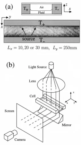
The apparatus is an evolution of the one described used by Daviaud and Vince.26 It consists of a rectangular con-tainer Lx long and Ly wide as shown in Fig. 1. Most of the
experiments have been carried out with Ly⫽250 mm and
Lx⫽10, 20, and 30 mm, and in some experiments, Ly has
been varied down to 30, 50, 75, 90, and 180 mm. For the
FIG. 1. Schematic drawing of the experimental apparatus.共a兲 Rectangular container: Cross section共top兲 and top view 共bottom兲. A liquid layer of depth h is subjected to a horizontal temperature gradient. The origin of coordinates is located on the hot side for x and at the bottom plate for z. 共b兲 Optical setup used to perform shadowgraphy.
range of fluid depths examined—1 mm⭐h⭐10 mm—these dimensions correspond to streamwise共resp. spanwise兲 aspect ratios 1⭐⌫x⫽Lx/h⭐30 共resp. 3⭐⌫y⫽Ly/h⭐250兲. The shorter walls are made of Plexiglas, while the two longer vertical walls are made of copper and are thermally regulated by circulating water at different temperatures T⫹ and T⫺. The lower boundary consists of a float glass plate and a Plexiglas plate is inserted a few millimeters above the sur-face of the fluid to reduce evaporation. With this configura-tion, the height of liquid remains constant to better than 1% over an experimental run. The same experiment was per-formed in an annular geometry with a gap between the inner cylinder and the outer cylinder being 10 mm and the mean perimeter 503 mm.32,36 In this last experiment, the main characteristics of the wave patterns are similar to those ob-tained in the rectangular geometry with Lx⫽10 mm.
The working fluid used is a 0.65 cSt Rhoˆne–Poulenc silicone oil whose physical properties are given in Table II. This liquid presents a low susceptibility to surface contami-nation, a medium Prandtl number P⫽10 and is transparent to visible light. Another fluid was used 共2 cSt silicone oil,
P⫽30兲 to check the existence of hydrothermal waves for
larger Prandtl numbers.
The fluid depth h is measured with a 0.05 mm precision and a meniscus is present at the boundaries. The horizontal temperature difference⌬T⫽T⫹⫺T⫺, is imposed by the two copper walls and is measured using thermocouples. This pa-rameter is regulated with a stability better than 2⫻10⫺2K. Room temperature is kept constant near 20°C and the hot and cold temperatures are adjusted so that the container mean temperature remains close to it.
The flow is characterized by temperature measurements and visualizations associated to image processing. Tempera-ture measurements are performed using a moving Cr–Al 共type K兲 0.25 mm thermocouple with a time response small enough to perform temporal temperature series with a 20 Hz maximal sampling rate. The accuracy of these measurements is typically 0.03 K. Shadowgraphy is used to control the perturbation of the flow due to the presence of the probe. We visualize the streamlines by sowing the flow with Merck Iriodin 100 Silver Pearl and by illuminating it with a He–Ne laser light sheet in different vertical planes. The patterns are also visualized by shadowgraphic imaging. A parallel verti-cal light beam crosses the container from top to bottom and forms a horizontal picture on a screen, due to surface defor-mations at the oil–air interface and to temperature gradients in the fluid. The surface deformations have been measured, looking at the deflection of a laser beam on the surface of the fluid. These measures give a deformation of less than 15m in agreement with the value of the capillary number Ca
⫽0.005 K⫺1⫻⌬T. As the surface deflection is small, the shadowgraphy method gives mainly the temperature gradient field variation.37
The spatio-temporal evolution of the structures is re-corded using a CCD video camera and the images are digi-tized to 256 gray levels along a line of 512 pixels perpen-dicular to the gradient. This method is described in detail elsewhere.26 Note that the observed region is limited to 185 mm by the optical setup. Some experiments have been per-formed in a Ly⫽180 mm reduced cell to avoid this
limita-tion. This will be indicated when needed. To extract the pat-tern behavior from the spatiotemporal diagrams, space and time Fourier transforms and complex demodulation tech-niques are used.33They allow a determination of the ampli-tude of the oscillations, the wave number, the frequency and thus the phase velocity.
FIG. 2. Stability diagram: temperature difference⌬Tcvs height of liquid h for共a兲 Lx⫽10 mm, 共b兲 Lx⫽20 mm, and 共c兲 Lx⫽30 mm. BF, TW, and SR, respectively, refer to basic flow, traveling waves, and stationary rolls. Verti-cal dashed lines correspond to the transitional depth hr.
TABLE II. Physical properties of Rhoˆne Poulenc silicone oil 0.65 cSt at 20 °C. Surface tension measurements have been performed by J. K. Platten at University of Mons-Hainaut共Belgium兲. Other properties are from the technical data sheet.
v
(m2/s) (kg/m 3) (K␣⫺1) (m2/s) 共N/m兲 ␥⫽⫺
/T
共N/mK兲 P
The two parameters which control our experimental sys-tem are h, the height of fluid in the cell, and ⌬T, the hori-zontal temperature difference between the two walls. In fact, one must keep in mind that, when varying h, ⌫x and⌫yare
also varied. The experimental procedure was the following: For a given Lx and height of fluid h, ⌬T is increased from
⌬T⫽0 by steps and we wait for t⫽30 min⬃100h2/at each step to allow the system to stabilize. Above the threshold, ⌬T is then decreased to study the existence of hysteresis. The steps are smaller than 0.5 K.
III. RESULTS
As soon as ⌬T⫽0, a convective flow is created. The thermal gradient across the cell induces a surface tension gradient on the free surface of the fluid. Because of the ther-mocapillary effect, this gradient generates a surface flow from the hot side towards the cold side, with a bottom recir-culation. Buoyancy forces also drives the flow in the same direction as thermocapillary forces. The basic flow appears thus as a long roll perpendicular to the gradient. In fact, depending on ⌫x and ⌬T, a unicellular or a multicellular
flow with transverse rolls can be observed共see below兲. This flow can then destabilize into different patterns, depending on the two parameters⌬T and h. The results are reported on the stability diagrams of Fig. 2 and show a dependence of the threshold values on Lxand h. The region named basic flow
共BF兲 accounts for both the steady unicellular and multicellu-lar flow. Depending on the height of liquid, two regimes occur. When ⌬T⭓⌬Tc(h), for small h values, the system
exhibits oblique traveling waves 共TW兲, while for larger h values, stationary longitudinal rolls 共SR兲 are observed. The value h⫽hrwhich separates TW from SR increases with Lx
共hr⫽2.7,3.6,4.0 mm for Lx⫽10,20,30 mm, respectively兲
while the threshold⌬Tc does not increase significantly. For
each h, the reported ⌬Tc value corresponds to the first
ob-served pattern that invades the whole cell. In the following, we first present the basic flow and then the different patterns observed while varying⌬T and h.
A. Basic flow
The basic flow has been characterized through tempera-ture measurements. Figure 3 presents the reduced horizontal temperature profiles ⌬T˜(r,t)⫽关T(r,t)⫺T⫺兴/⌬T obtained for Lx⫽20 mm and for different depths in two different
con-figurations: h⫽1.2 mm and h⫽3.2 mm. For h⫽1.2 mm, the temperature profile is linear and gives a mean temperature gradient measured in the center of the container H ⫽T/x which is of the order of the imposed temperature
gradienti⫽⌬T/Lx, i.e.,H⯝0.8i. Moreover, the profile is similar for all depths. This central temperature gradientH
defines for each depth h an effective temperature difference calculated as ⌬TH⫽H⫻Lx⬍⌬T. The difference between
effective and imposed temperature difference is due to the
FIG. 3. Reduced temperature⌬T˜⫽(T⫺T⫺)/⌬T vs x for different depths z for Lx⫽20 mm and ⌬T⫽3 K, below the onset of traveling waves. 共a兲 h ⫽1.2 mm, 共b兲 h⫽3.2 mm.
FIG. 4. Reduced temperature⌬T˜ vs x on the free surface for different h,
Lx⫽20 mm and ⌬T⫽3 K, below the onset of traveling waves.
FIG. 5. Vertical temperature profiles for different h for Lx⫽20 mm and ⌬T⫽3 K at x⫽10 mm 共middle of the container兲.具T典zdenotes the average of T over z.
presence of thermal boundary layers on both hot and cold sides. This effective gradient H allows direct comparisons with theoretical analysis by Smith and Davis3 and Mercier and Normand9who consider an infinite layer of fluid along x 共see below兲.
For h⫽4 mm, thermal boundary layers are much more important near the hot and cold walls and the measured temperature gradient is H⯝0.2i. A local inversion of
temperature can even be observed near the hot wall in the upper part of the fluid. This is an evidence of a roll in a narrow region near the hot wall.20,38 In fact, the ratio be-tween the measured and the imposed temperature gradient
H/i continuously decreases when the height of liquid is
increased 共Fig. 4兲. When h⭓6 mm, one can consider that there is no more temperature gradient in the middle of the cell; all the gradients take place in the vertical boundary layers.
The vertical temperature profiles obtained in the center of the cell for liquid layers with different height are pre-sented in Fig. 5. For small height (h⫽1.2 mm), the vertical gradient is small and uniform in z. When h increases, this gradient increases and becomes nonuniform along z: A mean vertical temperature gradientVcan be defined. For h above
3.2 mm, an inversion of the vertical gradient is observed in the upper part of the fluid layer. Globally, when h increases,
H decreases while V increases. For the smallest h 共resp.
highest兲 the gradient is nearly horizontal 共resp. vertical兲. For high h, due to the return flow, we observe a vertical tempera-ture gradient in the bottom of the cell. This profile is perhaps related to a downwards heat flux accross the glass bottom plate: Higher spatial resolution in the bottom boundary layer should be achieved to answer this question. The thermal boundary condition at the oil–air interface appears to be adiabatic for small h, while an upward-directed heat flux exists for greater h. This heat flux is at the origin of a sub-layer below the surface which is unstable against Be´nard– Marangoni type instability, the surface being colder than deeper in the fluid.
Depending on ⌬T and on the aspect ratio ⌫x, a
multi-cellular flow can be observed. As it was studied in details in
other works,14,19,28,37we do not report a detailed study of this instability. Let us mention that visualizations revealed this flow to correspond to corotating rolls. They appear near the hot wall and their number decreases when h increases 共⌫x
FIG. 6. Basic flow: Co-rotative rolls. 共a兲 Upper view for h⫽1 mm and ⌬T⫽6 K visualized with iriodin particles; 共b兲 horizontal temperature pro-files for h⫽2 mm and ⌬T⫽3 K. Inset: Temperature oscillations around the mean gradient in the gray marked region.
TABLE III. Hydrothermal waves: Critical⌬T and critical Marangoni numbers vs fluid depth h and dynamic Bond number Bo for Lx⫽10, 20, and 30 mm.
The Bond number has been computed with the classical definition: Bo(h)⫽(g␣/␥)h2. The Marangoni number has been computed with h and the global
thermal gradient⌬Tc/Lxfor the three values of Lxand also with the measured horizontal gradientHfor Lx⫽20 mm. The gradientHwas measured for
⌬T⫽3 K and 1.2⭐h⭐6 mm and the corresponding values have been interpolated.
Lx⫽10 mm Lx⫽20 mm Lx⫽30 mm h mm ⌬Tc K Bo(h) M a (⌬Tc/Lx,h) h mm ⌬Tc K H K•mm⫺1 Bo(h) M a (⌬Tc/Lx,h) M a (H,h) h mm ⌬Tc K Bo(h) M a (⌬Tc/Lx,h) 0.60 8.21 0.04 760 0.84 10.01 0.500 0.09 908 908 1.00 7.80 0.12 668 0.81 5.76 0.08 971 1.04 5.61 0.280 0.14 780 780 1.20 6.07 0.18 749 0.90 4.90 0.10 1020 1.24 4.25 0.177 0.19 839 698 1.44 4.40 0.26 782 1.10 3.77 0.15 1170 1.54 3.82 0.121 0.30 1170 736 1.98 4.30 0.49 1440 1.43 3.38 0.26 1780 1.80 3.43 0.089 0.40 1430 739 2.32 4.40 0.67 2030 1.70 3.55 0.36 2640 2.22 3.71 0.074 0.62 2350 932 2.74 4.30 0.94 2770 1.82 3.63 0.41 3100 2.50 3.98 0.068 0.78 3200 1090 3.16 4.40 1.25 3770 2.10 3.77 0.55 4280 3.00 4.29 0.058 1.12 4970 1340 3.36 4.54 1.41 4390 2.32 4.46 0.67 6170 3.50 5.76 0.064 1.53 9070 2010 3.64 4.60 1.65 5220 2.60 6.76 0.84 11700 3.80 5.00 1.80 6190 3.93 5.54 1.93 7330
decreases: 8 rolls for h⫽1 mm and Lx⫽20 mm, two rolls for
h⫽6 mm兲. These rolls can be visualized on an upper view of
the cell 共Fig. 6兲 and are observed as spatial oscillations on the horizontal temperature profiles. Different mechanisms have been proposed to account for this multicellular flow,9,13–15 but up to now, no complete answer has been given.
B. Traveling waves
Oblique traveling waves are observed for small depth layers (h⭐hr) for ⌬T⭓⌬Tc. ⌬Tc depends on h 共or Bo兲:
When increasing h, ⌬Tc decreases from small h towards a
minimum and then increases up to hr. The positions of the
minimum and of hr increase with Lx共Fig. 2 and Table III兲.
As soon as the threshold is crossed, two waves which propa-gate in opposite direction along the y axis, and towards the hot wall on the x axis appear in the container, separated by a source. The source shape and its evolution with ⌬T above the threshold depend of h.
The waves appear via a supercritical Hopf bifurcation: The frequency is finite at threshold1,23,26 –28 and the ampli-tude of the waves behaves as (⌬T⫺⌬Tc)1/2 共Fig. 7兲32,39,40
共see Table IV兲. Using the amplitude critical behavior, a more accurate threshold value can be obtained, smaller than the one given by the observation of spatio-temporal diagrams. In fact, for 1.5 mmⱗh⬍hr the transition for basic flow to
trav-eling waves invading the cell is relatively sharp, occuring within a few tenth of a degree. However, for smaller depths
of fluid, the oscillation that take place first are localized at the end boundaries. In order to study planar waves, we de-cided to report共Fig. 2, Table III兲 the onset in the long cells as the first state where the whole cell oscillates. This state can be as much as one or two degrees above the localized oscil-lation regime. This overestimation of the onset makes diffi-cult the comparison with theory and experiments in shorter cells27,28共see Discussion兲.
1. Wave sources
Depending on the fluid depth h, two different types of sources of waves can be distinguished:
共i兲 For smaller values of h (h⬍hc), the source looks like
a point located on the cold wall and emits a circular wave. Due to the confinement by the channel in the x direction, this wave becomes almost planar far from the source 共Fig. 8兲.
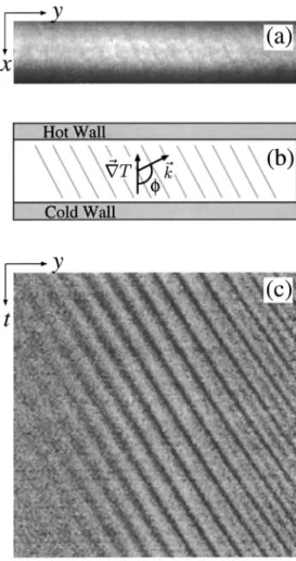
共ii兲 For higher h (hc⬍h⬍hr), the source looks like a line
parallel to the x axis and emits inclined planar waves. At onset, the pattern is symmetric and the source is in the middle of the channel.39 For ⌬T slightly above threshold—typically within 0.3 K—we observe the source to stand closer and closer to one end of the channel. Further from threshold, an asymptotic homo-geneous state is reached, where just a single wave is present. This state can be seen as a source at one end which emits a wave that dies in a sink at the opposite end共Fig. 9兲. The present Paper focuses especially on these homogeneous patterns.
The transition between these two behaviors is not sharp. We observe a crossover domain inbetween and the transition is hysteretic when varying h. To illustrate this phenomenon, let us describe a constant ⌬T⫽5.5 K experiment, i.e., slightly above onset, with h slowly decreasing in the Lx ⫽30 mm– Ly⫽180 mm cell.41This experiment is illustrated
in Fig. 10 by the position of the source 共a兲, the period 共b兲, and the wave number ky 共c兲 measured far from the source
and the transverse phase speed c⫽/ky 共d兲 which remains
nearly constant when h is varied. For h⬎hc⫽1.8 mm a
single traveling wave is emitted by a source at the extremity of the channel. For 1.5⬍h⬍1.8 mm the source leaves the extremity and transforms progressively into a circular
FIG. 7. Amplitude of the traveling waves vs ⌬T for h⫽1.7 mm, Lx
⫽10 mm, and Ly⫽180 mm. Experimental data (⫹) and fit A⫽(⌬T
⫺⌬Tc)1/2共solid line兲.
TABLE IV. Nondimensional characteristics of the hydrothermal waves for some depths just above threshold: Projection of the wave vector along y axis ky, frequency⫽2/T, and angle.
Lx⫽10 mm Lx⫽20 mm Lx⫽30 mm h 共mm兲 ky (1/h) (/h2) h 共mm兲 ky (1/h) (/h2) 共rad兲 h 共mm兲 ky (1/h) (/h2) 共rad兲 0.90 1.42 8.23 1.04 1.65 9.50 2.62 1.00 1.40 8.31 2.58 1.10 1.19 7.72 1.24 1.22 7.82 2.62 1.20 1.52 9.23 2.65 1.43 1.02 6.12 1.54 1.17 6.97 2.62 1.44 1.25 6.46 2.60 1.82 1.47 9.05 1.80 1.10 7.18 2.29 1.98 0.80 6.15 2.40 2.32 1.63 11.02 2.22 1.41 9.30 2.23 2.32 0.72 6.15 2.09 2.50 1.32 9.56 2.16 2.74 1.05 10.62 1.96 3.00 1.43 15.51 ⬃1.8 3.16 1.15 12.62 ⬃1.75 3.93 1.01 15.23 ⬃1.75
source. At h⫽1.5 mm, we observe a discontinuity of the wave number and frequency. Below this value the source is perfectly circular and continue to move towards the center of the channel. Finally the waves disappear at h⫽0.90 mm. The crossover between the two behaviors can be tracked on spa-tiotemporal data: For a source of circular waves, the projec-tion of the local wave vector along the y direcprojec-tion changes continuously from a negative value to a positive one when crossing the source; whereas for source of planar waves, we observe a superposition of waves with opposite wave num-ber ky. The superposition occurring in the latter case results
in the existence of standing waves共along y axis兲 in the core of the source. So we observed the amount of standing waves to smoothly decrease by a factor 10 when h decreases from 1.8 to 1.5 mm.41 When performing the reverse experiment and increasing h, the source remains located away from the extremities in a small hysteretic region above hc. No
sys-tematic study of this transition with parameters h and⌬T has been performed. We have observed that hc increases with
Lx: hc⫽1.1,1.6,1.8 mm for Lx⫽10,20,30 mm, respectively.
Other sources and sinks may even appear in the cell when strong increases of ⌬T are made, but they annihilate, leaving a single source. Far above ⌬Tc they may even
re-main stable, like frozen. The asymptotic behaviors described
above concern thus a narrow band above⌬Tc. Finally, in the
periodic annular channel—Lx⫽10 mm, Ly⫽503 mm—the
two types of sources are also observed above and below hc,
but only during transients; sources and sinks are both un-stable near onset always leaving a single wave. We can thus conclude about the stability of defects that sources are stable at small heights in the rectangular container and sinks are always unstable except at the extremities of the channel.
The two types of sources reported above can be related to the two types of hydrothermal waves observed in a larger aspect ratio experiment.37,40However, in our very long rect-angular channel, the two type of wave can only be differen-tiated close to the source.
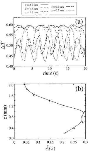
2. Temperature oscillations measurements
Temperature measurements reveal that the traveling waves correspond to bulk temperature oscillations. As shown in Fig. 11, the corresponding temperature evolution for a defined position x0 can be described as Tx
0(z,t)
⫽A˜(z)cos(Tt)⫹
具
T(x0,z)典
, where T is the frequency ofthe oscillation, identical to that measured with shadowgraphy
, A˜ (z) is the amplitude of the oscillation for each depth and
具
T(x,z)典
denotes a time-average of the temperature signal inFIG. 8. Traveling waves, h⬍hc.共a兲 Shadowgraphic image and 共b兲
sche-matic drawing of the pattern in an horizontal plane;共c兲 spatiotemporal evo-lution for Lx⫽30 mm, Ly⫽250 mm, h⫽1.6 mm, and ⌬T⫽5.6 K. The field
of view corresponds to⬃185 mm.
FIG. 9. Traveling waves, hc⬍h⬍hr. 共a兲 Shadowgraphic image and 共b兲
schematic drawing of the pattern in an horizontal plane;共c兲 spatiotemporal evolution for Lx⫽30 mm, Ly⫽250, h⫽3.00 mm, and ⌬T⫽4.64 K. The
a given spatial position (x,z). This amplitude is less than 0.5 K, and its z-dependence can be seen in Fig. 11共b兲.
The maximum of the amplitude of the oscillations is reached at middle-depth (z⯝h/2), and the minimum at the surface (z⫽h). This kind of behavior was predicted by Smith5and experimentally observed in another configuration by Pelacho et al.28 This temperature behavior is compatible with the proposed hydrothermal wave instability mecha-nisms, which is responsible of the up-flow component of the wave number.
3. Characteristics of the waves at threshold
The waves behave as plane waves near the threshold, i.e., an unique wave number and frequency can describe their evolution. As the wave propagates from the cold to the hot side, the x component kxis negative in our referential, and ky is positive 共resp. negative兲 for the right 共resp. left兲 traveling
wave. As a consequence, k forms an angle共see schematics in Figs. 8 and 9兲 with the x axis, varying between/2⬍ ⬍.
When we change the experimental parameters, the wave number k, the angleand the frequency evolve. For the three values Lx⫽10,20,30 mm two regions can be
distin-guished:
共i兲 For hⱗhc(Lx), the wave number ky and the
fre-quencydecrease with h while the angle has a nearly constant value⬃0.83⫽2.6 rad 共Fig. 12兲. Note that if we define the angle with the gradient as ␣⫽ ⫺, his value is approximatively␣⬃/6.
共ii兲 For hcⱗh⬍hrthe frequency increases with h, but the
angle decreases until a value ⫽0.64⬃2 rad 共␣ ⬃/3 for large h, Fig. 12兲. The wave number ky
in-creases slightly for hⲏhc and saturates when
ap-proaching hr.
The different characteristics of the waves for some val-ues of h are summarized in Table IV.
4. Influence of the aspect ratio
To evaluate the influence of the aspect ratio⌫y⫽Ly/h or
⌫⫽Ly/Lx on the instability, various experiments were
real-FIG. 10. Evolution with varying h at⌬T⫽5.5 K for Lx⫽30 mm and Ly ⫽180 mm. 共a兲 y position of the source in the cell. 共b兲 Period T of the wave. 共c兲 Projection of the wave vector kyaway from the source.共d兲 Projection of the phase velocity c⫽/kyalong y .
FIG. 11. Traveling waves for h⫽2 mm and ⌬T⫽6 K. 共a兲 Evolution of the reduced temperature⌬T˜ with time at different depths z. 共b兲 Amplitude A˜(z) of the waves vs depth z.
ized for 0.75⬍h⬍2.75 mm and various Ly between 30 and
90 mm, leaving Lx⫽30 mm constant, i.e., for horizontal
as-pect ratio ⌫ from 1 to 3.
For small height, between 0.75 and 1 mm, we observe for ⌫⬃1, 2, and 3 the waves to nearly propagate along the direction of the thermal gradient from cold side to hot side. This corresponds mainly to the core of point sources as de-scribed in Sec. III B 1. A perfectly symmetric point source for
Ly⫽90 mm is shown in Fig. 13.
For higher height, between 1.75 and 2.75 mm, we ob-serve for ⌫⬃1 (Ly⫽30 mm) and ⌫⬃3 (Ly⫽90 mm),
pla-nar waves to propagate obliquely from cold side to hot side along x axis and both side along y axis. Such behavior re-calls precisely the observations in longer cells. However, for
Ly⫽50 mm, h⫽2.75 mm, and ⌬T⫽5.8 K⬎⌬Tc, we report an inverse dynamics. Traveling waves are observed which propagate from the hot to the cold side, along the gradient direction, and are reminiscent of those observed by Ezersky
et al.21,22and Garcimartı´n et al.20
Thresholds have been measured for Ly⫽90 mm to be
just a few tenth of a degree above those presented above for long channels. A discussion concerning the different thresh-olds measurement methods is presented in Sec. IV C. For shorter cells, no accurate measurements have been carried out but the threshold appears generally above those for longer channel configuration. This finite size effect as been recently studied by Pelacho et al.42
Let us note that for small aspect ratio cells the relative importance of menisci with respect to the bulk grows. For low h especially, because⌬Tcis very high, oscillatory
insta-bilities appear in the menisci for ⌬T below the hydrothermal-waves onset in the bulk.
C. Stationary rolls
For h⬎hr the basic flow destabilizes in the form of a
stationary pattern with a wave vector perpendicular to the horizontal applied gradient. At threshold, the pattern appears only near the hot side and invades the rest of the cell when ⌬T is increased. A typical shadowgraphy of the cell is shown in Fig. 14. These stationary patterns correspond to the desta-bilization of the primary roll in the y direction as in Be´nard– Marangoni convection. The wave number associated with this pattern remains nearly constant (k⯝3.2) for a large range of values of hⲏhr and increases slowly for larger h
共Fig. 15兲.
Using iriodin particles, we have visualized the flow in-side these convective cells: It consists in a superposition of a circulation in the xz plan due to the basic flow and a con-vective circulation in the y z plan for each cell due to bulk induced convection. The walls of each cell are well defined,
FIG. 12. Traveling waves just above threshold: Evolution of共a兲 the wave number ky,共b兲 the frequency⫽2/T,共c兲 the angle, as a function of h. Experimental data 共dotted lines兲: 共䉭兲 Lx⫽10 mm, 共䊐兲 Lx⫽20 mm, (⫹) Lx⫽30 mm. Theoretical predictions: 共dashed line兲 Smith and Davis 共Ref. 3兲; 共〫 and solid line兲 Mercier and Normand 共Ref. 9兲.
FIG. 13. Shorter cell: Shadowgraphy snapshot for h⫽1.0 mm, Lx
⫽30 mm, Ly⫽90 mm (⌫⫽3) and ⌬T⫽7.3 K. The cold side is down. This
nearly circular wave propagates from the point source located in the middle of the cold side. Menisci are very important in distorting the sides of the pattern outside the cell. The whole cell is visible.
FIG. 14. Stationary rolls, h⫽6 mm, ⌬T⫽6 K, Lx⫽30 mm. Shadowgraphic
and the fluid does not cross them. In a convective cell, be-cause of the primary roll flow, the fluid moves upwards near the hot wall, and downwards near the cold wall.
For intermediate x, the observation of independent cells along the y axis allows to describe the temperature profiles in Fig. 16 as two superimposed layers consisting of counter-rotating rolls. Because of the convective flow, the fluid cir-culates in the y z plan, ascending in some places, and de-scending in others. These recirculations induce temperature modulations along the z direction inside the upper (2⬍z ⬍6 mm) and lower (0⬍z⬍2 mm) layers 共Fig. 16兲. An iso-therm (z⬃2 mm) separates both layers.
The vertical temperature profile below onset共Fig. 5兲 ex-hibits two layers: An upper layer near the surface which is unstable with respect to Be´nard–Marangoni criterion and a lower layer with stable thermal stratification. Linear stability analysis of uniformly heated layer of depth d predicts a non-dimensional wave number k⬃2 in Be´nard–Marangoni convection.43In the d⫽2h/3 upper layer, this would lead to
k⯝3, close to the k⫽3.2 measured value. D. Further from threshold
Further from threshold, the different patterns destabilize: 共i兲 At small depth hⱗhc, we observe series of traveling
holes33 to be shed continuously in the intermediate
regions located between the circular source and the planar-wave regions. Whereas there is almost no de-fect near onset, their number increases with ⌬T 共cf. Fig. 2 of Burguete et al.33兲.
共ii兲 For intermediate depth, hcⱗh⬍hr, we report the
oc-currence of a secondary instability in the shape of modulational instability of the single-wave-pattern. This instability is similar to Eckhaus instability but occurs with low but finite wave number. We observe spatially growing wave number-modulations which eventually lead to regular shedding of spatio-temporal dislocations in the cell. This patterns are quasiperiodic in both frequency and space. Downstream the dislo-cations, a lower-wave number pattern is observed, which is either monoperiodic or chaotic owing to h and Lx. These results will be reported elsewhere.
共iii兲 For large depth h⬎hr, the stationary pattern has a
secondary instability in the form of an oscillation in phase-opposition共optical mode, Fig. 17兲 with a finite frequency at threshold. This behavior has been ob-served in similar steady pattern for other convection experiments: Rayleigh–Benard convection in narrow gap,44 and in nonuniform heating,45 where a fluid layer is heated from the bottom with a nonuniform temperature profile.
E. Higher Prandtl number fluid
Finally, a restricted set of experiences using a P⫽30 (⫽2 cSt) fluid has been realized to evaluate the influence of the Prandtl number. At h⫽2.0 mm no hydrothermal waves were observed up to ⌬T⫽30 K. For h⬎3 mm, stationary rolls where observed. According to available experimental results in shallow horizontal 共rectangular or annular兲 layers hydrothermal waves have not been reported above P⫽17. This annular experiment in ethanol23 has shown hydrother-mal waves as well as surface waves depending of h.
Never-FIG. 15. Stationary rolls: Evolution of the wave number k as a function of the depth of liquid h at threshold (⌬T⫽⌬Tc).
FIG. 16. Stationary rolls: Horizontal reduced temperature profiles⌬T˜ vs y for different depths z for x⫽10 mm, h⫽6 mm, and ⌬T⫽10 K. Those pro-files have not been recorded simultaneously and might be shifted.
FIG. 17. Spatiotemporal evolution for stationary rolls: Optical mode for Lx⫽20 mm, h⫽4 mm, and ⌬T⫽13 K far from threshold.
theless Priede and Gerbeth10 predicted waves up to P ⫽1000. We believe this prediction to be correct, but it is experimentally very difficult to produce the critical gradient. The higher the Prandtl number, the sharper the temperature variation in the thermal boundary layers at both extremities: The effective horizontal gradient H keeps small even for
high⌬T.
IV. DISCUSSION
A. Relevant parameters
1. Spatial scales and Bond number
The experimental data show the existence of two transition depths hc and hr. These depths separate three regions where different forces dominate. For small h, surface stresses are dominant and no vertical stratification has been observed 共Fig. 5兲. Buoyant effects are small. Above
hc, buoyant forces are no more negligible, and the
tempera-ture profile varies with z 共Fig. 5兲. Finally, above hr the
buoyant forces dominate and the thermal gradient is almost vertical.
The stability diagrams—minima positions, hc, hr 共Fig.
2兲—and the characteristics of the waves and of the stationary rolls—k, f , 共Figs. 12 and 15兲—move towards larger depths when Lx increases. We tried to reduce the data for
different h and Lx. The natural idea is to plot the data vs the
Bond number Bo⫽Ra/Ma. With the classical reduction9—
⫽⌬T/Lx and d⫽h—the Bond number varies as h2 and
does not reduce the data. Other combinations of h and Lx
have been tested and h3/Lxgives the best results: All these
curves collapse into single ones共Figs. 18 and 19兲. In particu-lar the transition between hydrothermal waves and stationary rolls occurs for hr3/Lx⫽2.1⫾0.2 mm2.
As far as the Bond number is believed to be the relevant parameter for this flow, our experimental results impose Bo to be a function of h3/Lx. A very simple way to obtain this is
to build the Marangoni number using exclusively the hori-zontal scale Lx and the Rayleigh number using exclusively
the depth h M a
冉
⌬T Lx ,Lx冊
⫽ ␥⌬TLx , Ra冉
⌬T h ,h冊
⫽ g␣⌬Th3 .The Bond number is then
Bo共h,Lx兲⫽ g␣ ␥ h3 Lx .
For the transitional depth hr, we compute Bo(hr,Lx)
⫽0.25 showing buoyant and capillary forces to be of the same order of magnitude.
2. Thermal gradient
Let us note that even if the experiment control parameter is the horizontal temperature difference ⌬T this study has shown the necessity to measure both horizontal and vertical effective gradients H and V to understand the instability
mechanisms.
FIG. 18. 共a兲 Stability diagram in reduced coordinates: Effective horizontal temperature difference⌬TH⫽HLxvs h3/Lxfor different Lx. Evolution of 共b兲 the wave number ky,共c兲 the frequency⫽2/T, and共d兲 the angleas a function of h3/L
x.
FIG. 19. Stationary rolls: Evolution of the wave number k at threshold as a function of h3/Lx.
3. Biot number
In infinite layer theoretical studies, the Biot number is used to control the vertical temperature profile. In our experi-ment, the temperature profiles have been measured and shown to vary along x. Also, the air layer is typically 1 cm thick and is, therefore, animated by strong convective flows. These two effects make it impossible to calculate an exact value of Bi. It could be possible to measure it from very careful measurement of the temperature field in the air very near the fluid surface.
Using our data, the only possibility is to compare the heat flux across the free surface from vertical temperature profiles共Fig. 5兲: The effective Biot number increases with h.
B. Comparison with theoretical results 1. Hydrothermal waves
In this section, we will compare our measurements with different theoretical results. We will use the classical defini-tions of Marangoni and Bond numbers, M aTh and BoTh
M aTh⫽Ma
冉
⌬T Lx ,h冊
⫽ ␥ ⌬Th2 Lx , BoTh⫽g␣ ␥ h2.Furthermore, as far as theoretical studies concern only planar waves, we compare them with experimental data collected far from the sources where waves are planar whatever h.
Because the thermocapillar effects dominate for small h, we expect the results obtained by Smith and Davis3,4,11 to describe our experimental results. The nondimensional char-acteristics predicted by Smith and Davis for the return flow using a fluid with P⫽10 and Bi⫽0 can be summarized as: Wave number 兩k兩⬃2.5, propagation angle ⬃160°, fre-quency ⬃0.14 and phase velocity c⬃0.06. It is important to note that the time unit used by Smith and Davis is
/␥H. These waves appear for a critical Marangoni
num-ber M acTh⫽300.
Let us consider the case Lx⫽30 mm. 共The data
pre-sented in Table IV for Lx⫽10 or 20 mm give similar results.兲
For h⬍hc, a very good agreement with SD is found. For
example, for h⫽1.00 mm, and using the Smith and Davis time unit definition, the experimental values are 兩k兩⫽2.6,
⫽150°, ⫽0.14, and c⫽0.05. Nevertheless, the experi-mental critical Marangoni number value is M acTh⫽668. This value is larger than the predicted value but corresponds to the invasion of the whole cell by the waves. We studied the first occurence of waves in shorter cells allowing a complete vi-sualization and plot the observed threshold in the ( M a, Bo) plane in Fig. 20. We report M aTh⫽434 for the same depth with Ly⫽180 mm. The variation of the critical Marangoni
number with Bo is in very good agreement with the pre-dicted limit M acTh⫽300 for Bo⫽0.
On the other side, for h⫽2.74 mm⬎hc, the wave appear
for M acTh⫽2800 which reduces to 840 when based on the estimated effective horizontal temperature gradientH. The
experimental characteristics of the waves above onset are: 兩k兩⫽1.1, ⫽110°, ⫽0.18, and c⫽0.16. A discrepancy is found for兩k兩,andbetween the experimental values and these values predicted by SD.
Mercier and Normand9共MN兲 have considered the effect of bulk forces. For h⬃1 mm 共small Bo兲 their results are similar to SD. For BoTh⫽1 (h⫽2.83 mm), P⫽7 and Bi ⫽1 they report Mac⫽386. Using as time unit h
2/, they found: k⬃2.5, ⬃100°, ⬃19, c⬃7. Using this time unit, the experimental values for h⫽2.74 mm become: k⫽1.1,
⫽110°, ⫽11, c⫽9. The angle and the phase speed are well recovered while the wave number differs by a factor of 2. In Fig. 12, we show the theoretical data from the Mercier and Normand predictions, Smith and Davis prediction, which does not depend on h, and the experimental data. Qualita-tively, a similar behavior is found between the MN values and the experimental ones when h is varied. Nevertheless, a quantitative comparison fails, mainly because of the wave number values, which are always smaller共typically one half兲 in the experiment. Two reasons can explain this difference. The first one is the finite size of the experimental cell be-cause it can influence the basic flow even far from the cell walls. This effect is not considered in the numerical analysis. The second one is the discrepancy found between the experi-mental and numerical temperature z-profiles below the threshold共Fig. 5 and MN兲.
2. Nonlinear behavior
Smith performed a nonlinear stability analysis11 of the SD solutions. He predicted the traveling wave 共resp. mixed
FIG. 20. Critical Marangoni M a(⌬Tc/Lx,h) number vs dynamic Bond number Bo(h). Open squares stand for Lx⫽30 mm and Ly⫽250 mm data reported in Table III. The closed squares stands for a measurement in the
Lx⫽30 mm and Ly⫽180 mm cell and the open circles for the Lx⫽30 mm and Ly⫽90 mm cell. Open triangles stand for Riley and Neitzel’s data 共Ref. 27兲 in Lx⫽30 mm and Ly⫽50 mm cell and closed triangles stand for Pela-cho and Burguete’s data共Ref. 28兲 in Lx⫽60 m and Ly⫽50 mm cell. See text for details.
wave兲 solution to be stable 共resp. unstable兲 for P⫽10. We confirm this prediction for h⬎hc, reporting a single inclined traveling-wave. However, for h⬍hc, the shape of the source
deserves a two-dimensional description41which has not been made as far as we know.
3. Stationary rolls
Stationary patterns for this buoyant-thermocapillary problem have been predicted by Mercier and Normand.9 Ac-cording to Fig. 1共b兲 of MN, two unstably stratified layers can develop near the surface and the bottom plate for positive
Bi. The above layer destabilizes against Be´nard–Marangoni
instability whereas the bottom layer can be Rayleigh–Be´nard unstable. This calculation, made for a bottom plate with a fixed linear temperature gradient, predicts the bottom layer to be thicker and to transit first.
In our system, the vertical temperature profile is unstable only in the upper layer共Fig. 5兲. This difference can be due to the finite conductivity of the glass bottom plate and thus to possible heat flux across.
C. Comparison with experimental results in large rectangular channels
Experiments in large rectangular containers with similar horizontal gradient have been performed by Riley and Neitzel27 共RN兲 and by Pelacho and Burguete28 共PB兲. Both experiments use Ly⫽50 mm, a much smaller value than
ours. Onset values have been plotted in Fig. 20 together with our results for Lx⫽30 mm and various Ly. The data for Lx
⫽10 and 20 mm are not represented 共cf. Sec. IV A 1兲. All data exhibit the same evolution with Bond number. The only discrepancy concerns the lowest value of Bo 共small h兲 for our data in Table III. This discrepancy has been noted by RN and is explained by the fact that the waves solution at thresh-old are strongly inhomogeneous in our long cell. This is reinforced by our choice to report onset only when the whole cell is invaded, in order to compare with the uniform theo-retical solution. Complementary studies have considered shorter Ly⫽90 mm and Ly⫽180 mm cells where the first
apparition of waves is reported as onset. Onsets are much lower for small h and in perfect agreement with RN and PB data共Fig. 20兲. Let us note that the main characteristics of the waves are close to RN and PB data. We also found compa-rable values for the effective gradient near oscillation thresh-old for RN data (0.75⬍h⬍1.75). Riley and Neitzel present two oscillating modes: Hydrothermal waves 共HTW兲 for h ⬍1.3 mm and oscillarory multicellular cells 共OMC兲 above. In our longer cell, we clearly observe the hydrothermal waves to superimpose on steady corotating rolls along y axis.37 We believe that RN’s oscillatory multicellular cells also represent this combination.
V. SUMMARY AND CONCLUSION
Experimental results obtained in a lateral heating experi-ment have been presented. Varying the experiexperi-mental param-eters h, Lx, Ly, and ⌬T, various stable states have been
characterized. The basic flow that appears as soon as ⌬T is not null, can be destabilized producing hydrothermal waves 共for h⬍hr兲 or stationary rolls (h⬎hr).
The observed hydrothermal waves correspond to bulk temperature oscillations, and exhibit different behaviors de-pending on the value of h. For h⬍hc, the surface stresses
are dominant, and the characteristics of the planar waves are very close to those predicted by Smith and Davis.3 For h ⬎hc, their description is no more applicable because of the
vertical temperature gradients that appear across the fluid layer, amplifying buoyancy effects. For these values of h, the predicted results of Mercier and Normand,9including buoy-ant forces, are recovered except the wave number value. The quantitative discrepancy could be due to finite size consider-ations that alter the vertical velocity and temperature profiles. The spatial structure of the wave pattern reveals two types of wave-sources depending on the fluid depth. We believe these sources to trace back the existence of two different types of waves: one-dimensional waves for h⬎hc and
two-dimensional waves for h⬍hc.
37,40
For large h, when buoy-ant forces dominate, the basic flow destabilizes in the form of a stationary pattern, which can be related to Be´nard– Marangoni convection.
This set of experiments brought many quantitative data varying most control parameters of the system. In trying to reduce the set of relevant parameters, we emphasize the role of h3/Lxas the spatial scale of the problem. This parameter appears in a natural way when the Bond number is expressed using a Marangoni number based on horizontal scale Lxand
a Rayleigh number based on vertical scale h.
ACKNOWLEDGMENTS
The authors thank M. A. Pelacho, A. Garcimartı´n, H. Mancini, C. Pe´rez-Garcı´a, J. F. Mercier, and C. Normand for stimulating discussions and C. Gasquet, M. Labouise, and B. Ozenda for their technical assistance. We also thank J. K. Platten for the measurement of the oil surface tension. J.B. acknowledges a postdoctoral grant from SEUID 共Spanish Government兲 and financial support through contracts PB98-0208 共Spanish Government兲 and PIUNA 共Universidad de Navarra, Spain兲.
1F. Preisser, D. Schwabe, and A. Scharmann, ‘‘Steady and oscillatory
ther-mocapillary convection in liquid columns with free cylindrical surface,’’ J. Fluid Mech. 126, 545共1983兲.
2M. C. Cross and P. C. Hohenberg, ‘‘Pattern formation outside of
equilib-rium,’’ Rev. Mod. Phys. 65, 851共1993兲.
3M. K. Smith and S. H. Davis, ‘‘Instabilities of dynamic thermocapillary
liquid layers. Part 1. Convective instabilities,’’ J. Fluid Mech. 132, 119 共1983兲.
4
S. H. Davis, ‘‘Thermocapillary instabilities,’’ Annu. Rev. Fluid Mech. 19, 403共1987兲.
5M. K. Smith, ‘‘Instability mechanisms in dynamic thermocapillary liquid
layers,’’ Phys. Fluids 29, 3182共1986兲.
6P. Laure and B. Roux, ‘‘Linear and non-linear analysis of the Hadley
circulation,’’ J. Cryst. Growth 97, 226共1989兲.
7G. Z. Gershuni, P. Laure, V. M. Myznikov, B. Roux, and E. M.
Zhukho-vitsky, ‘‘On the stability of plane-parallel advective flows in long horizon-tal layers,’’ Microgravity Q. 2, 141共1992兲.
8
insta-bilities in medium-Prandtl number fluid layers subject to a horizontal tem-perature gradient,’’ Int. J. Heat Mass Transf. 36, 2417共1993兲.
9J. F. Mercier and C. Normand, ‘‘Buoyant-thermocapillary instabilities of
differentially heated liquid layers,’’ Phys. Fluids 8, 1433共1996兲.
10J. Priede and G. Gerbeth, ‘‘Convective, absolute and global instabilities of
thermocapillary-buoyancy convection in extended layers,’’ Phys. Rev. E
56, 4187共1997兲.
11M. K. Smith, ‘‘The nonlinear stability of dynamic thermocapillary liquid
layers,’’ J. Fluid Mech. 194, 391共1988兲.
12B. M. Carpenter and G. M. Homsy, ‘‘Combined buoyant-thermocapillary
flow in a cavity,’’ J. Fluid Mech. 207, 121共1989兲.
13H. Ben Hadid and B. Roux, ‘‘Buoyancy and thermocapillary-driven flows
in differentially heated cavities for low Prandtl number fluids,’’ J. Fluid Mech. 235, 1共1992兲.
14D. Villers and J. K. Platten, ‘‘Coupled buoyancy and Marangoni
convec-tion in acetone: experiments and comparison with numerical simulaconvec-tions,’’ J. Fluid Mech. 234, 487共1992兲.
15J. F. Mercier and C. Normand, ‘‘Influence of the Prandtl number on the
location of recirculation eddies in thermocapillary flows,’’ Int. J. Heat Mass Transf.共in preparation兲.
16
M. Mundrane and A. Zebib, ‘‘Oscillatory buoyant thermocapillary flow,’’ Phys. Fluids 6, 3294共1994兲.
17J. Xu and A. Zebib, ‘‘Oscillatory two- and three-dimensional
thermocap-illary convection,’’ J. Fluid Mech. 364, 187共1998兲.
18
R. Velten, D. Schwabe, and A. Scharmann, ‘‘The periodic instability of thermocapillary convection in cylindrical liquid bridges,’’ Phys. Fluids A
3, 267共1991兲.
19C. De Saedeleer, A. Garcimartı´n, G. Chavepeyer, J. K. Platten, and G.
Lebon, ‘‘The instability of a liquid layer heated from the side when the upper surface is open to air,’’ Phys. Fluids 8, 670共1996兲.
20A. Garcimartı´n, N. Mukolobwiez, and F. Daviaud, ‘‘Origin of surface
waves in surface tension driven convection,’’ Phys. Rev. E 56, 1699 共1997兲.
21
A. B. Ezersky, A. Garcimartı´n, J. Burguete, H. L. Mancini, and C. Perez-Garcia, ‘‘Hydrothermal waves in Marangoni convection in a cylindrical container,’’ Phys. Rev. E 47, 1126共1993兲.
22A. B. Ezersky, A. Garcimartı´n, H. L. Mancini, and C. Perez-Garcia,
‘‘Spa-tiotemporal structure of hydrothermal waves in Marangoni convection,’’ Phys. Rev. E 48, 4414共1993兲.
23D. Schwabe, U. Mo¨ller, J. Schneider, and A. Scharmann, ‘‘Instabilities of
shallow thermocapillary liquid layers,’’ Phys. Fluids A 4, 2368共1992兲.
24J. Schneider, D. Schwabe, and A. Scharmann, ‘‘Experiments on surface
waves in dynamic thermocapillary liquid layers,’’ Microgravity Sci. Tech-nol. 9, 86共1996兲.
25M. K. Smith and S. H. Davis, ‘‘Instabilities of dynamic thermocapillary
liquid layers. Part 2. Surface-waves instabilities,’’ J. Fluid Mech. 132, 145 共1983兲.
26
F. Daviaud and J. M. Vince, ‘‘Traveling waves in a fluid layer subjected to a horizontal temperature gradient,’’ Phys. Rev. E 48, 4432共1993兲.
27R. J. Riley and G. P. Neitzel, ‘‘Instability of thermocapillary-buoyancy
convection in shallow layers. Part 1. Characterization of steady and oscil-latory instabilities,’’ J. Fluid Mech. 359, 143共1998兲.
28M. A. Pelacho and J. Burguete, ‘‘Temperature oscillations of hydrothermal
waves in thermocapillary-buoyancy convection,’’ Phys. Rev. E 59, 835 共1999兲.
29Y. Kamotani, J. Masud, and A. Pline, ‘‘Oscillatory convection due to
com-bined buoyancy and thermocapillarity,’’ J. Thermophys. Heat Trans. 10, 102共1996兲.
30
P. Gillon and G. M. Homsy, ‘‘Combined thermocapillary-buoyancy con-vection in a cavity: An experimental study,’’ Phys. Fluids 8, 2953共1996兲.
31
M. G. Braunsfurth and G. M. Homsy, ‘‘Combined thermocapillary-buoyancy convection in a cavity. Part II. An experimental study,’’ Phys. Fluids 9, 1277共1997兲.
32N. Mukolobwiez, A. Chiffaudel, and F. Daviaud, ‘‘Supercritical Eckhaus
instability for surface-tension-driven hydrothermal waves,’’ Phys. Rev. Lett. 80, 4661共1998兲.
33
J. Burguete, H. Chate´, F. Daviaud, and N. Mukolobwiez, ‘‘Hydrothermal wave amplitude holes in a lateral heating convection experiment,’’ Phys. Rev. Lett. 82, 3252共1999兲.
34J. M. Vince and M. Dubois, ‘‘Hot wire below the free surface of a liquid:
structural and dynamical properties of a secondary instability,’’ Europhys. Lett. 20, 505共1992兲.
35
E. Favre, L. Blumenfeld, and F. Daviaud, ‘‘Instabilities of a liquid layer locally heated on its free surface,’’ Phys. Fluids 9, 1473共1997兲.
36N. Mukolobwiez, ‘‘Etudes de systemes d’ondes propagatives dans de
ecoulements thermogravitaires et thermocapillaires,’’ Ph.D. thesis, Univer-site´ Paris XI, France, 1998.
37N. Garnier, ‘‘Ondes non lineaires a une et deux dimensions dans une
mince couche de fluide,’’ Ph.D. thesis, Universite´ Paris 7, France, 2000.
38D. Schwabe and H. Du¨rr, ‘‘Holographic interferometry and flow
visualiza-tion by tracers applied to buoyant-thermocapillary convecvisualiza-tion in an open rectangular gap,’’ Microgravity Sci. Technol. 9, 201共1996兲.
39N. Garnier and A. Chiffaudel, ‘‘Non-linear transition to a global mode for
traveling-wave instability in a finite box,’’ Phys. Rev. Lett. 86, 75共2001兲.
40N. Garnier and A. Chiffaudel, ‘‘Two dimensional hydrothermal waves in
an extended cylindrical vessel,’’ Eur. Phys. J. B 19, 87共2001兲.
41N. Garnier, A. Chiffaudel, and F. Daviaud, ‘‘Transition 1D-2D pour des
ondes hydrothermales non-line´aires,’’ in 2e`me Rencontre du Non-line´aire IHP Paris 1999, edited by Y. Pomeau and R. Ribotta共Paris Onze Editions, Orsay, 1999兲, pp. 193–198 共in French兲.
42M. A. Pelacho, A. Garcimartı´n, and J. Burguete, ‘‘Local Marangoni
num-ber at the onset of hydrothermal waves,’’ Phys. Rev. E 62, 477共2000兲.
43J. R. A. Pearson, ‘‘On convection cells induced by surface tension,’’ J.
Fluid Mech. 4, 489共1958兲.
44M. Dubois, R. Da Silva, F. Daviaud, P. Berge´, and A. Petrov, ‘‘Collective
oscillating mode in a 1D chain of convective rolls,’’ Europhys. Lett. 8, 135 共1989兲.
45
J. Burguete, ‘‘Inestabilidades producidas por un calentamiento local-izado,’’ Ph.D. thesis, Universidad de Navarra, Spain, 1995.


![[PDF] Cours C 2 Types entrees sorties de base et structures de controle | Cours langage c](data:image/gif;base64,R0lGODlhAQABAIAAAP///wAAACH5BAEAAAAALAAAAAABAAEAAAICRAEAOw==)