A dimension reduction technique to preserve nearest neighbors on high dimensional data

(1)

A Dimension Reduction Technique to Preserve

Nearest Neighbors on High Dimensional Data

by

Christos Nestor Chachamis

B.S., Massachusetts Institute of Technology (2019)

Submitted to the Department of Electrical Engineering and Computer

Science

in partial fulfillment of the requirements for the degree of

Master of Engineering in Electrical Engineering and Computer Science

at the

MASSACHUSETTS INSTITUTE OF TECHNOLOGY

May 2020

c

○ Massachusetts Institute of Technology 2020. All rights reserved.

Author . . . .

Department of Electrical Engineering and Computer Science

May 18, 2020

Certified by . . . .

Samuel Madden

Professor

Thesis Supervisor

Accepted by . . . .

Katrina LaCurts

Chair, Master of Engineering Thesis Committee

(2)

(3)

A Dimension Reduction Technique to Preserve Nearest

Neighbors on High Dimensional Data

by

Christos Nestor Chachamis

Submitted to the Department of Electrical Engineering and Computer Science on May 18, 2020, in partial fulfillment of the

requirements for the degree of

Master of Engineering in Electrical Engineering and Computer Science

Abstract

Dimension reduction techniques are widely used for various tasks, including visualiza-tions and data pre-processing. In this project, we develop a new dimension-reduction method that helps with the problem of Approximate Nearest Neighbor Search on high dimensional data. It uses a deep neural network to reduce the data to a lower dimension, while also preserving nearest neighbors and local structure. We evaluate the performance of this network on several datasets, including synthetic and real ones, and, finally, we compare our method against other dimension reduction techniques, like tSNE. Our experiment results show that this method can sufficiently preserve the local structure, in both the training and test data. In particular, we observe that most of the distances of the predicted nearest neighbors in the test data are within 10% of the distances of the actual nearest neighbors. Another advantage of our method is that it can easily work on new and unseen data, without having to fit the model from scratch.

Thesis Supervisor: Samuel Madden Title: Professor

(4)

(5)

Acknowledgments

First and foremost, I would like to thank my supervisor, Sam Madden, for giving me the opportunity to work together on this project and providing me with funding, great ideas, and amazing support for the last year.

I also would like to thank Lei Cao for providing me with help, ideas, and solutions whenever needed. His inputs and technical help were crucial to my research and allowed me to overcome any challenges in the project.

In addition, I am forever grateful for my family for providing me with everything I need to succeed in life. They are a source of constant hope and endless support. My love for science and engineering is due to them. I would like to thank my friends and MIT for making my college years a very rewarding and memorable experience, along with making me feel welcome in this new home. I would like to thank two people in particular: Andriana Velmahos for being by my side and supporting me and Dimitris Koutentakis for being a great friend.

Last but not least, I would like to thank George and Christos Kalivas for providing me with a safe haven during the pandemic. Their kindness allowed me to focus on my research, during a very frightening and threatening time.

(6)

(7)

Chapter 1 Introduction

1.1 Introduction

The purpose of this project is to invent a new method that we believe can be helpful in solving the problem of approximate nearest neighbor search in high dimensional data.

Nearest neighbor search is a well studied problem in the field of machine learning. It can be very useful, and it has a number of applications. There is a vast amount of data like text, images or audio, so there is an ever increasing need of being able to identify the most similar object to a given query. Some examples would include finding the movie most similar to another movie, the song most similar to a given audio file or the topic most related to a text. In cases like these, we turn the objects, for instance text, into high dimensional data, by using feature extraction techniques relative to the specific task, e.g. Word2Vec for text. Then, we perform the task of finding the nearest neighbor from a certain database, that is, the object in the database most similar to the query object. In the text example, that would mean finding the text or document that is most similar to a target document. In this project we ignore the process of turning the objects into numbers and focus only on the method for nearest neighbor search, as applied on the high dimensional data.

We start by defining the problem of Nearest Neighbor Search (NN search). Sup-pose that the inputs come from the space R𝐷. Let 𝑥𝑖 ∈ R𝐷 be the available data

(12)

points, which are going to serve as points in the training data set. Let 𝑑 : R𝐷× R𝐷 _→

R be a distance function and 𝑞 ∈ R𝐷 a data-point for which we want to per-form a query. The problem of the nearest neighbor search is to identify the point 𝑥*(𝑞) = argmin_{𝑖∈{1,...,𝑁 }}𝑑(𝑞, 𝑥𝑖).

The above task is particularly difficult when the input data come from a high-dimensional space (𝐷 larger than 20 and ofetn in the range of hundreds or thousands, as is typical for image and audio representations), due to a problem called the curse of dimensionality. The curse of dimensionality states that in high dimensions, i.e. above 20, there is little difference in the distances between different pairs of samples. Thus, heuristics like the triangle inequality cannot be effectively used [Li+16].

Because of the curse, most methods for nearest neighbor search fail to perform better than a linear scan, which is considered inefficient due to the number of distance calculations needed. As a result, researchers have focused on the problem of approx-imate nearest neighbor search (ANN search), that is, finding a neighbor that is close enough to the true nearest neighbor. In this project, we design a new method that can be useful when doing ANN search for both low-dimensional and high-dimensional data.

There are many reasons for studying high-dimensional data. First, data in high dimensions is widely used in real applications. Physical objects, like images or biolog-ical data, are quite complex, so we need a lot of attributes to represent them in a way that captures their structure and properties well. Restricting one to low dimensions would mean that a lot of information is lost or not used. The applicability of high dimensional data makes the problem much more challenging and interesting to solve. In addition, no definite solution has been found for the problem of nearest neighbor search in high dimensions, mostly due to the curse of dimensionality. Solutions exist for the problem of searching data in low dimensions, especially when the Euclidean distance is used. Instead, when dealing with high-dimensional data, people tend to study the problem of Approximate Nearest Neighbor Search instead.

Approximate Nearest Neighbor (ANN ) search is the problem of identifying neigh-bors that are quite close to the query object, though not necessarily the closest ones.

(13)

This approximation is a convenient compromise. Most of the time, an object which is “close” to the query object is good enough for practical purposes, while numerous approaches for ANN search have been found and studied. In this project, we study a method that can be useful when tackling the problem of ANN. We hope that it can act as a nice transformation that lowers the dimensions of the input points, without sacrificing a lot of the information.

Through our method, we utilize the power of deep learning networks to transform the data into points in which the approximate nearest neighbor search is easier to solve. That is, we aim to develop a model that is good in preserving neighbors. This resembles other dimension reduction techniques, like tSNE. Contrary to these methods however, we want a method that can easily work with and adapt to new data. tSNE is not efficient in reducing unseen data, as it needs to re-train on all data again. In this project, we investigate how well we can do with a general neural network and several different loss functions. We then perform several tests to see which parameters and methods work the best.

1.2 Background and Related Work

The problem of nearest neighbor search is a well studied one. This is especially true for the problem of search on low-dimensional data.

1.2.1 ANN Search Methods

There is a vast literature devoted on the problem of nearest neighbor search, especially for the case of approximate nearest neighbor search. Here, we don’t solve the problem of ANN search specifically, but we touch on it, so we think it is helpful to present some of the state of the art techniques.

One of the most popular type of methods is locality sensitive hashing (LSH). LSH was introduced by Indyk and Motwani. The basic idea of LSH is to use random pro-jections to reduce the dimension of the input space, and then discretize the points and add them in a hash table. The search algorithm proceeds by reducing the dimension

(14)

of the query and finding the nearest neighbor in the appropriate bucket. Probabilis-tic proofs guarantee efficiency in the average case. The main disadvantage of LSH methods is that they are completely data-independent.

Another type of ANN search method is space-partitioning. Typically, such meth-ods produce trees that divide the input space based on clusters or distances from data points. The search then recursively visits trees and nodes until no improvement can be made.

Finally, other techniques studied in the literature are graph-based methods. Such methods create graphs representing the local structure (nearest neighbors or nearest cluster of points) of the data points, together with some of the global structure of the points. Then, the search algorithm is a greedy search from random points until no nearest points can be found.

1.2.2 Dimension Reduction Techniques

Dimension reduction is a problem directly related to this research, as this is the learning task we try to solve. The most novel techniques in the dimension reduction literature are tSNE [MH08] and UMAP [MH18]. They are both very similar in nature, and what sets them apart from each other are some differences in the choice of cost and similarity function. Both of these methods produce results that are exceptionally good qualitatively. The main disadvantage of these methods is that they cannot map unseen points to the lower dimension space, without rerunning the whole optimization algorithm. In our approach however, we learn a neural network function, so it is easy to map the unseen input points to output points. Although our method is more updateable than these techniques, they serve as excellent benchmark on how a good dimension reduction should look like.

Another method that is worth mentioning is PCA [Pea01]. PCA is different than the methods mentioned above, as it tries to find the dimensions that are worth keeping for maintaining most information. PCA does not differentiate between local and global structure, all information is treated the same.

(15)

sophisti-cated. In principle, tSNE guesses the output points and then uses some optimization method (like gradient descent) to improve on the guesses. On the contrary, we are trying to create a mapping of the whole space. Instead of guessing output points, we learn a deep network that does the reduction, and then use optimization methods to improve the mapping.

(16)

(17)

Chapter 2 Model

In this Chapter, we describe the specifics of our models. We assume that the data comes from a fixed but unknown distribution, so we use a machine learning model to identify the distributions of the data. We explain how fitting the model is per-formed and what the exact parameters of the machine learning model are. Finally, we examine different variations of the machine learning model.

2.1 General Model

The general model consists of a deep linear neural network NET, called the reducer, that takes a high-dimensional data point in R𝐷_{, where 𝐷 is usually in the range of}

hundreds or thousands, and maps it to a reduced-dimension data point in R𝑀, where 𝑀 should be a small number, like 10. The objective of the reducer is to preserve the nearest neighbors of every point when the points are mapped to their low-dimensional counterparts. In this project, we aim to show that the reducer NET can preserve the local distances. This property can then be utilized to store the training data to find the lower dimensions and perform quick searches on the nearest neighbors of the queries.

(18)

2.2 Distance and Similarity

Intuitively, we would like the local distances in the output space R𝑀 to resemble as much as possible the local distances in the input space R𝐷_{. In addition, distant}

points should be relatively far from each other, so that they are not included in the nearest neighbor count. Even though we defined the problem in terms of distances, we are going to feed the model NET with similarities. Similarities have some desirable properties compared to distances. They are bounded between 0 and 1, so they are easier to work with. In addition, similarities have a natural interpretation in terms of probabilities; the more similar the points, the more probable it is that they are going to be close to each other. Turning distances into probabilities is an easy task. Let 𝑑 : R𝑛_{× R}𝑛 _{→ R}

≥0 be the distance function. Some possible similarity functions

𝜎 : R𝑛× R𝑛_{→ [0, 1] are:}

1. Cosine Similarity:

𝜎(𝑥, 𝑦) = 𝑥 · 𝑦 ‖𝑥‖2· ‖𝑦‖2

This is valid when the distance 𝑑 is the Euclidean distance

2. Exponential Similarity: 𝜎(𝑥, 𝑦) = exp{︁−1 2𝑑(𝑥, 𝑦) 2}︁ 3. Inverse Similarity: 𝜎(𝑥, 𝑦) = 1 1 + 𝑑(𝑥, 𝑦)2

In practice, we did not observe any difference between the exponential and the inverse similarity, so we are using a variant of the inverse similarity for our model. In addition, the inverse function seems easier to work with compared to the exponential. In either case, we can use any distance metric for the choice of the function 𝑑, though we focus only on the Euclidean distance in this project. Note that in both cases we consider the square of the Euclidean distance, so we don’t have to consider the square root calculation in the computations and the performance becomes more efficient.

(19)

As described above, we want to match the input and output distances in order to create a meaningful reduction. However, it is important to note that the distance, or rather the similarity functions in the input and output spaces need not be the same. One intuition for that is that in the input space the distribution of the distances might take any special form related to the data. We are not interested in preserving this form (for example the specific variance) but it is more suitable to preserve the ranking of the distances related to each point. Then, the definition of similarity in the output space could be the general inverse similarity defined above, but for the input space it seems more suitable to use a similarity function that simplifies the distance distributions.

Let 𝑑in : R𝐷× R𝐷 → R≥0 be the Euclidean distance in the input space. We define

the input similarity 𝜎in: R𝐷 × R𝐷 → [0, 1] as

𝜎in(𝑥𝑖, 𝑥𝑗) = [︃ 1 + 𝜖 + 𝑑in(𝑥𝑖, 𝑥𝑗) 2_{− 𝑑}2 𝑖 𝑑2 𝑖 ]︃−1 = _𝑑 1 in(𝑥𝑖,𝑥𝑗)2 𝑑2_𝑖 + 𝜖 , for 𝑗 ̸= 𝑖,

where 𝜖 is a small constant and 𝑑𝑖 = min𝑗̸=𝑖{𝑑(𝑥𝑖, 𝑥𝑗)}, that is, 𝑑𝑖 is the minimum

distance of a point from 𝑥𝑖. For completeness, we define 𝜎in(𝑥𝑖, 𝑥𝑖) = 1. The similarity

𝜎in(𝑥𝑖, 𝑥𝑗) is inversely proportional to distance 𝑑in(𝑥𝑖, 𝑥𝑗). The maximum similarity

possible is 𝜎max = (1 + 𝜖)−1. If we hadn’t made the correction step of subtracting

and dividing by the minimum distance squared, then the similarity could potentially be very small, even for the close neighbors. Observe that 𝜎max is the maximum

similarity for any point, and for every point there exists another point that makes their similarity equal to 𝜎max. It is worth noting that when fitting the model we

do not know in advance what 𝑑𝑖 is, so we need to take this into consideration while

fitting.

In terms of the output similarities, there is no need to consider any scaling up or down, since the model can place the points in the R𝑀 _{space freely. Thus, we consider}

(20)

𝜎out : R𝑀 × R𝑀 → [0, 1]

𝜎out(𝑦𝑖, 𝑦𝑗) =

1

1 + 𝑑out(𝑦𝑖, 𝑦𝑗)2

,

where 𝑦𝑖 and 𝑦𝑗 are the outputs 𝑦𝑖 = NET(𝑥𝑖) and 𝑦𝑗 = NET(𝑥𝑗) respectively. As

before, 𝜎out(𝑦𝑖, 𝑦𝑗) is inversely proportional to 𝑑out(𝑦𝑖, 𝑦𝑗). In contrast to the input

similarity, the output one is symmetric.

2.3 Loss Function

Let 𝜎in and 𝜎out be the input and output similarity functions, as defined above.

Given the data points 𝑥𝑖, 𝑖 = 1, 2, . . . , 𝑛, we fit the model NET to minimize the

KL-divergence between input and output similarities, together with a sum of squared errors as a regularization factor. That is, our objective is

ℒ(𝑦1, 𝑦2, . . . , 𝑦𝑛; 𝑥1, 𝑥2, . . . , 𝑥𝑛) = ∑︁ 𝑖,𝑗 𝑝𝑖𝑗log (︁𝑝_𝑖𝑗 𝑞𝑖𝑗 )︁ + 𝜆∑︁ 𝑖,𝑗 (𝑝𝑖𝑗 − 𝑞𝑖𝑗)2,

where 𝑞𝑖𝑗 is the input similarity

𝑞𝑖𝑗 =

𝜎in(𝑥𝑖, 𝑥𝑗) + 𝜎in(𝑥𝑗, 𝑥𝑖)

2 ,

and 𝑝𝑖𝑗 is the output similarity

𝑝𝑖𝑗 = 𝜎out(𝑦𝑖, 𝑦𝑗) = 𝜎out(NET(𝑥𝑖), NET(𝑥𝑗))

is the similarity of the output points 𝑦𝑖 and 𝑦𝑗.

The KL divergence ∑︀ 𝑖,𝑗𝑝𝑖𝑗log (︁ 𝑝𝑖𝑗 𝑞𝑖𝑗 )︁

is a natural candidate for the loss function for two reasons. First, KL divergence loss is designed to make probabilities match each other. We can conveniently think of similarities 𝑞𝑖𝑗 and 𝑝𝑖𝑗 as the probabilities of

points 𝑥𝑗 and 𝑥𝑖 to be close to each other. Then, fitting in this sense would preserve

(21)

pairs of points that are close to each other in input space and predicted to be far in output space, than pairs of points that are far from each other and predicted to be close. This is a desirable property, because we are more interested in keeping close points together, than distant points apart.

The way we defined similarities 𝜎in means they are asymmetric, since 𝑑2𝑖 and 𝑑2𝑗

can be different, so we take the extra step of defining 𝑞𝑖𝑗 as the average of the two

similarities to make the input to the loss function symmetric. We do this to make sure that our results are more accurate. The idea behind it is to make the final result less susceptible to outliers. Imagine a point 𝑥 that is far away from a cluster of points. The nearest neighbor of 𝑥 is a point 𝑘 in the cluster. Then, input similarity 𝜎in(𝑥, 𝑘)

is 𝜎max = (1 + 𝜖)−1, even though the points are far away. We would like to be able to

capture this difference. We might miss the nearest neighbor of 𝑥, but there will be less noise in creating the neighborhood of 𝑘.

Finally, the sum of squared errors works as a regularization of the loss, which is the KL Divergence. We will discuss more about this in Chapter 6. In short, the regularization helps to keep the points more tightly together. Without regularization, or with a small value of 𝜆, the points tend to make clusters that form lines on the output space. On the other hand, a larger value of 𝜆 would make the points form regularly formed clusters (without assuming a clear structure, e.g, a line), and be closer to each other. The larger the value of 𝜆, the tighter the clusters are. It is not clear to us why this pattern appears. It might have something to do with the fact that the squared error (𝑦𝑗− 𝑦𝑖)2 has a local minimum when 𝑦𝑖 = 𝑦𝑗, that is, when all

the points are mapped to the same output.

2.4 Training

Fitting the model is a rather straightforward task, once a few points have been re-solved. First, it is impractical to go over every pair of points. That would be quadratic in the number of points and it is prohibiting with a large number (millions) of them. Instead, we iterate over all points for a given number of epochs and perform constant

(22)

time operations. For every iteration and for every point 𝑥𝑖, we choose a second point

𝑥𝑗 at random, different from 𝑥𝑖. Let the similarities 𝜎in and 𝜎out, and the quantities

𝑝𝑖𝑗 and 𝑞𝑖𝑗 be as defined in Chapters 2.2 and 2.3. Then, we optimize for the objective:

ℓ(𝑥𝑖, 𝑥𝑗) = 𝑝𝑖𝑗log

(︁𝑝_𝑖𝑗 𝑞𝑖𝑗

)︁

+ 𝜆(𝑝𝑖𝑗 − 𝑞𝑖𝑗)2

Since 𝑝𝑖𝑗 = 𝜎out(NET(𝑥𝑖), NET(𝑥𝑗)), we can update the weights of NET by

back-propagation. In order to calculate the quantity 𝑞𝑖𝑗 we need the values of 𝑑2𝑖 and 𝑑2𝑗.

Of course, we do not have these values, as they are equivalent to solving the original problem. However, we can keep track of the shortest squared distances found so far and use those instead. When we calculate 𝑑(𝑥𝑖, 𝑥𝑗)2 we compare it with 𝑑2𝑖 and 𝑑2𝑗

and update any of the two values that is larger than 𝑑(𝑥𝑖, 𝑥𝑗)2.

As we fit the model, we use a small validation set to inspect the performance of the model per epoch. This does not contribute to fitting (for example by terminating when some condition is met). We use it to inspect how the performance is affected per epoch. The validation set needs to be small so that it is feasible to perform the exact nearest neighbor search.

2.5 Parameters

There is a number of parameters we need to specify for the project. The first is the architecture of the network. Since this is a project in which we try to evaluate the performance of a method, rather than beat some benchmark, we did not explore too many options. We chose an architecture with 3 hidden layers. The first layer has size 500, the second layer has size 100, and the third layer has size 20. In most of this project we use an output dimension of 10, though in Chapter 6 we reduce to R2 _in

order to facilitate plotting of the results. We choose 10 as a number small enough to solve the problem of nearest neighbor search but large enough to preserve most of the useful information of the input space.

(23)

parameters of Pytorch. In practice, we observe little value added after the first few epochs, so we can choose a number as low as 10 − 20. Finally, we choose the values 𝜆 = 1 and 𝜖 = 0.1 for the similarities and the loss function.

2.6 Model Variations

Much of the research for this paper has focused on different variations of the model described above. One of the most important components of the model is the loss function. Later, we will explore how different loss functions behave and how they affect the performance. It might be the case that some loss function that the authors have not tested has a better performance on preserving the nearest neighbors. How-ever, the loss function described in Chapter 2.3 is the one with the best performance, so we present the results based on this one.

(24)

(25)

Chapter 3 Data

In this Chapter we describe the datasets used in our experiments. This is a project in which we investigate the performance of a method, rather than beating a benchmark. Thus, we simply generated most of the data. Then, if the model works well, we can extend the project into using real-life datasets. The size of the datasets needs to be large, so that there are enough points for the network to be able to learn. In addition, the dimension needs to be high, by definition of the problem. However, we also perform analysis on a real dataset.

3.1 Clustered Synthetic Data

The first dataset consists of 100, 000 points divided into ten clusters. The dimension of each point is 200. This is the dataset we use to compare the performance of different variations of the model (see Chapter 6) and compare the performance of the model versus tSNE (see Chapter 5.4). When the dataset is used for training, we randomly select 90, 000 points that serve as the training set, and randomly select 1, 000 different points that serve as the validation set. With 1, 000 points, the problem of finding the exact nearest neighbors is feasible, and it takes about one minute using our implementation on our machine.

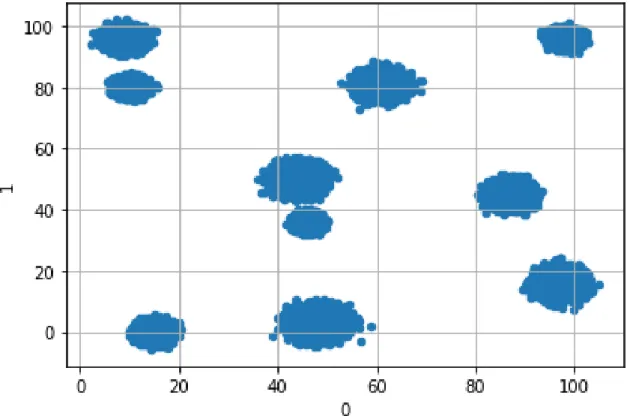
During data generation, we selected the centers of the ten clusters at random. The range for each coefficient is [0, 100]. For every point to be generated, we choose one

(26)

of the clusters at random, and we sample from a normal distribution with the chosen center of the cluster as the mean of the distribution and a random diagonal matrix as the covariance matrix of the distribution. The covariance matrix is fixed for every cluster, but it is otherwise random. Below we have plotted the first two dimensions of the dataset.

Figure 3-1: Plotting of first two coefficients for the Clustered Synthetic Data.

3.2 Large Clustered Synthetic Data

One of the reasons for using a model that can reduce unseen points is for scale. When we see a really large dataset, we can train the model on only a subset of the data and then reduce the remaining points as well. For this reason, we use a large dataset of 1, 000, 000 points. The method for generating is the same as the one described in the previous subsection. The dimension is 200 and the points belong to one of ten clusters. The dataset is used in Chapter 5.5 to investigate how the method works when we do sub-sampling.

(27)

3.3 Clustered Synthetic Data with Noise

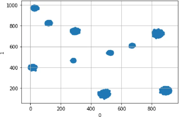
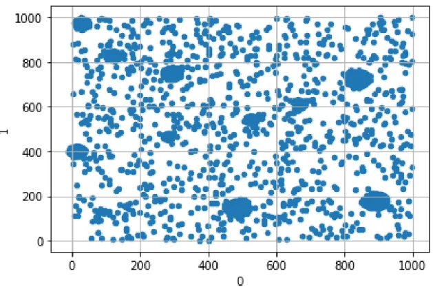
So far, the data we have used contain one very obvious pattern (the clusters), which can be discovered by other methods, like tSNE. For this reason, it would be useful to examine a dataset with some noise as well as some clear patterns. We start by generating 100, 000 points divided in ten clusters, in the same way as the one we described in Chapter 3.1. In order to have more sparse noise, we choose every coefficient to be in the range [0, 1000], instead of [0, 100]. Then, we draw 1, 000 points at random from [0, 1000]200_{. This is the noise. For training, we choose 99, 000 points}

from the clustered data at random and add the 1, 000 noisy points. This means that 1% of the train data have no clear pattern. We also choose the 1, 000 points left as the validation dataset.

Below we can see the plot of the first two dimensions of the new data, with and without noise.

Figure 3-2: Plotting of first two coefficients for the Clustered Synthetic Data, before the addition of noise.

(28)

Figure 3-3: Plotting of first two coefficients for the Clustered Synthetic Data with noise.

3.4 Uniform Synthetic Data

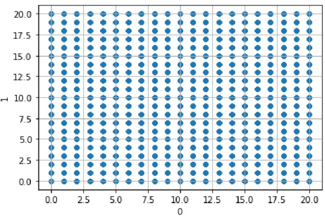
Finally, we want to see what happens if we have a truly random dataset, in which there is no obvious pattern for the model to learn. In order to generate the data, we draw 200, 000 points uniformly at random from the domain {0, 1, . . . , 100}200. Note that the coefficients in this case are integers. We do not have any special reason to restrict ourselves only to integers, besides wanting to test how the network learns in a more discrete setting.

Below we can see a plotting of the data for the first two coefficients in the range [0, 20] × [0, 20]. We can see that every point with integer coefficients is included. This is reasonable, since there are 200, 000 points in total, but only 10, 000 pairs of coefficients in the two dimensions.

(29)

Figure 3-4: Plotting of first two coefficients for the Uniform Synthetic Data.

3.5 Real Data

We use two real datasets in this project. The first one is the SIFT dataset, formally introduced in [JDS11]. It includes 1 million vectors of dimension 128. Besides the vectors used for training, there are two additional datasets, one with 10, 000 queries, and one which contains the groundtruth real neighbors of the queries among the 1 million base vectors. The second dataset contains the MNIST data [LeC+98], a set of 60, 000 images of handwritten digits. It has become a standard dataset used in dimension reduction and visualization studies, so we are going to use it as well for comparing our method with tSNE later in the project.

(30)

(31)

Chapter 4 Methods and Metrics

In this Chapter we discuss how we evaluate the performance of the model. We are primarily interested in qualitative features (things we can see in graphs), correctness and efficiency.

4.1 Qualitative Features

One of the most frequently used datasets in this project is the Clustered Synthetic Data (Chapters 3.1 and 3.2). We know in advance that random samples of this dataset are roughly going to be divided in ten clusters. When the local structure is preserved, we would expect that the number of clusters is preserved as well. Thus, one way to immediately make sure that some experiment produces reasonable results is to inspect the plotted data of the output space. We would expect that there is some pattern similar to the pattern of the input data.

4.2 Correctness

The most important objective of this method is how well the local distances are preserved in the output space. We want the points in the output space to have roughly the same neighbors as they did in the input space. We have identified two kinds of tests to help us evaluate at what degree the above objective is true.

(32)

4.2.1 Out-of-sample Reduced Dataset Tests

For the first method, we reduce a whole test dataset, hence the term out-of-sample. In the reduced space, we analyze the relations of the test data points with each other. In particular, we start by counting how many of the nearest neighbors in the reduced points correspond to the actual nearest neighbors. When we use the term actual in this research we mean the quantities that correspond to the input space, since they are the ground truth we are trying to match.

In addition, our approach resembles more the approximate nearest neighbor search, rather than the exact search. The nearest neighbor might not be the one closest to the reduced point, but still very close. In this case, we are trying to see how many of the actual nearest neighbors are in the top 5, 10 or 20 of the nearest neighbors in the reduced space.

Finally, we would like to know how off from reality are the nearest neighbors. That is, we are looking for a way to compare the actual distances of the actual nearest neigh-bor and the nearest neighneigh-bors in the reduced space. Let 𝑥𝑖 ∈ R𝐷 be a point in the

input space. Let 𝑦𝑖 = NET(𝑥𝑖) be the reduced point, 𝐴𝑖 = argmin𝑥𝑗̸=𝑥𝑖{𝑑in(𝑥𝑖, 𝑥𝑗)}

the actual nearest neighbor and 𝐵𝑖 = argmin𝑥𝑖,𝑥𝑗{𝑑out(NET(𝑥𝑖), NET(𝑥𝑗))} the

near-est neighbor of 𝑦𝑖 in the reduced space. Then,

𝑅𝑖 =

𝑑in(𝐵𝑖, 𝑥𝑖)

𝑑in(𝐴𝑖, 𝑥𝑖)

− 1

shows how close the two points are. By definition, the above quantity is non-negative, with equality to 0 when the actual nearest neighbor is guessed correctly. Once training is over, we observe and report the distribution of {𝑅𝑖 : 𝑖 = 1, . . . , 𝑛}.

This method of testing is quite ambitious, as it trains the model on one set and tests it on another, in which the points and the nearest neighbors are totally different.

4.2.2 Query Test

A more natural method of testing is looking for the nearest neighbors of the test data in the training dataset. The idea is that the model does a good job in reducing the

(33)

input dataset, so reducing points that are close to the original points should also be reliable. This method consists of reducing a dataset of queries and searching for the nearest neighbors in the reduced training data.

Let 𝑄 = {𝑞𝑗 : 𝑗 = 1, . . . , 𝑚} be the query data and 𝑋 = {𝑥𝑖 : 𝑖 = 1, . . . , 𝑛} be the

train data. Let 𝐴𝑗 = argmin𝑥𝑖{𝑑in(𝑞𝑗, 𝑥𝑖)} be the actual nearest neighbor of 𝑞𝑗, and

let 𝐵𝑗 = argmin𝑥𝑖{𝑑𝑜𝑢𝑡𝑝(NET(𝑞𝑗), NET(𝑥𝑖))} be the reduced nearest neighbor of 𝑞𝑗.

Then, we perform the same analysis we do on the out-of-sample reduced data test. We count how many of the 𝐴𝑗’s and 𝐵𝑗’s correspond, that is, how many of the nearest

neighbors are preserved after the transformation. We do the same thing for the top 5, 10 and 20 nearest neighbors in the reduced space, as described in Chapter 4.2.1. Finally, we report the distribution of

𝑅𝑗 =

𝑑in(𝐵𝑗, 𝑞𝑗)

𝑑in(𝐴𝑗, 𝑞𝑗)

− 1,

that is, the distribution of how far the reduced nearest neighbor is from the actual nearest neighbor.

4.3 Efficiency

Another important metric we care about is time efficiency. As mentioned earlier, solving the problem of exact nearest neighbor search takes a very long time, actually quadratic in the number of points. In addition, other methods, like tSNE, also take a large amount of time when we need to reduce a large amount of data. The method we have developed needs to run only once, for training, so we might be able to allow some more time for it. Even with that in mind, we still want it to be quite fast. Thus, we also measure the time it takes to finish training. Note that it is infeasible to run the exact nearest neighbor search or tSNE for large amounts of data, so we omit those calculations altogether.

(34)

(35)

Chapter 5 Results

In this Chapter we present the results obtained by testing the model on the methods introduced in Chapter 4. We start by training and testing the model on the several datasets mentioned in Chapter 3, with the exception of the large clustered dataset, which is to be used in the Chapter related to scaling. In the first two parts we test the correctness and time aspects of the method. Then, we investigate the results on using different values for the parameters. In particular, we see how the 𝜆 parameter of the loss function and the number of epochs affect the performance of the model.

In order to simplify the task of testing different parameter values, we keep the choice of dataset fixed. In particular, we test for 𝜆 and number of epochs by using the Clustered synthetic dataset, and assume that the trends will be similar for the other datasets. Especially for the number of epochs, testing only for one datasets is necessary, since testing takes some non-negligible amount of time, which becomes large when done for each epoch individually.

5.1 Results Per Dataset

Here we discuss how the method has performed in the 4 datasets mentioned above. The tests and methods used are the ones introduced in .

(36)

5.1.1 Clustered Synthetic Data

We start by investigating the performance of the model in the dataset of the clustered synthetic data. As we discussed above, this dataset is the main focus of our research. It contains some clear patterns that can be learned by the model, so any method that we wish that can bring results should do some reasonable performance on this dataset.

After fitting the model, we can observe in Figure 5-1 the reduced training space forming ten clusters. In addition, we observe the same ten-clustered pattern formed in the reduced test space (Figure 5-2). This means that every point in the test space is assigned to the correct cluster, and hopefully it is close to its actual nearest neighbors. The method has the ability to learn the more macro-behavior of the input space and passes the basic qualitative test of reducing the whole space, as described in Chapter 4.

Figure 5-1: Output of trained model on the clustered train data.

Figure 5-2: Output of trained model on the clustered validation data.

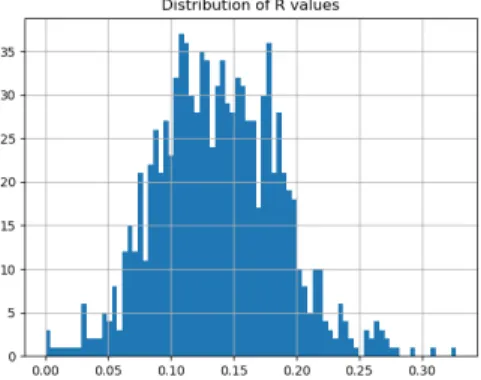
Next, we reduce the test space and investigate how close the test points are mapped relative to the other points. In Figure 5-3 we can see the histogram for the relative distances between the actual and predicted nearest neighbors for each target point. There are some interesting properties in this graph. First, there is a spike in zero, which means that a lot of nearest neighbors are predicted correctly. Then, the mean and the bulk of the distribution is around 0.10. The fact that most predicted shortest distances are up to 10% away from the real shortest distances means that the model

(37)

can be used successfully in an ANN setting.

In Figure 5-4 we can observe a similar result. This graph shows the histogram of the relative distances between the predictive and actual shortest distances when the test data are used as queries, and the input data are used as the database from which we draw the neighbors. Now there is no spike near zero, which means that most predicted nearest neighbors are incorrect. Still, the mean of the distribution is between 15% and 20%, which is a promising result for the query test.

Figure 5-3: R-distribution for the clus-tered data case.

Figure 5-4: R-distribution for the test queries in the clustered data case.

1 5 10 20

Clustered 22 (2.2%) 106 (10.6%) 216 (21.6%) 380 (38%) Table 5.1: Nearest Neighbors for the out-of-sample test. Test size is 1000.

Finally, we can see the loss function starting from a very negative value in the beginning and then converging to the −10, 000 value. The loss function converging in a negative value is a pattern common to all tests done for this project. It indicates that the input similarities are in general larger than the output similarities. This follows from the fact that the input similarities are found in the denominator of the log in the KL divergence.

What is the reason for this asymmetry? One explanation might be that the in the input similarities we use the ratios of the actual distances with the minimum distance, so this creates an artificial discount. In addition, we use the same small constant for

(38)

all closest distances, even if the points are far from each other. The input similarities do not form probability distributions, since we would have to somehow normalize to 1. Still, it should not matter that input similarities are artificially larger than what they should be, as the transformation still preserves the order and relative distances.

Figure 5-5: Loss function per epoch of training.

5.1.2 Clustered Synthetic Data with Noise

For the next experiment, we use the same dataset as above, in which we add some noisy points, that is, points that were generated at random with no specific pattern in mind. For more details the reader can visit Chapter 3.3. We train the model with this new dataset and see how the performance changes, on the same test dataset as the one used above.

In the figures below we see the first two dimensions of the reduced train and test spaces. The output space of the train data seems rather uniform. However, this

(39)

happens because the noisy data are added. In the reduced test space we clearly see the ten clusters of points.

Figure 5-6: Output of trained model on clustered train data with noise.

Figure 5-7: Output of trained model on clustered validation data.

Below, we can see the R-distribution of the noisy clustered data. Similar to the distribution in the above subsection, there is a large spike close to zero, and then the large mass is around 0.10. However, we can observe fatter tails and more skew.

Figure 5-8: R-distribution for the noisy clustered data case.

Figure 5-9: R-distribution for the test queries in the noisy clustered data case.

1 5 10 20

Noisy 18 (1.8%) 91 (9.1%) 187 (18.7%) 321 (32.1%)

(40)

Finally, the loss function seems to stabilize but it has some differences with the loss function of the above. In particular, it starts from positive and it decreases, until it stabilizes to a negative value.

5.1.3 Uniform Data

One of the datasets on which we train the model is on uniform data. When we say uniform, we mean that the data were generated by selecting for every coefficient a uniformly random number within a certain range (for more details see Chapter 3.4). The idea for using this dataset is that there is no clear pattern for the model to learn, but rather the data look like a cloud.

Below are the results for training the model on the uniform dataset. The training lasted for 20 epochs and the output dimension of the model was 20. We can observe

(41)

some striking differences compared to the results of the previous datasets. In the first figures we see the plot of the first two coefficients. Similarly to the input space, there is no apparent pattern in the data, besides a large cloud. The points in the train and test sets are in the same region of the space.

Figure 5-11: Output of trained model on uniform train data.

Figure 5-12: Output of trained model on uniform validation data.

The quantitative results are similar. In the 𝑅 distribution we can observe that the mean and median are larger compared to the values found in previous parts, while the spike that is usually located on zero is now missing. This is translated to two facts. First, the reduced neighbors are farther away relative to the the actual neighbors, compared to the other datasets studied. Second, not many actual nearest neighbors are preserved. For the latter, Table 5.3 is demonstrative.

Figure 5-13: R-distribution for the uniform data case.

Figure 5-14: R-distribution for the test queries in the uniform data case.

(42)

1 5 10 20 Uniform 2 (0.2%) 9 (0.9%) 14 (1.4%) 33 (3.3%)

Table 5.3: Nearest Neighbors for the out-of-sample test. Test size is 1000.

In addition, the loss function of the had a different trend compared to the previous datasets. In the previous datasets there was the trend of the loss function to getting closer to 0, forming a graph that resembled a convex function. On the other hand, we can see here the loss function going on the opposite direction, while making a graph that looks like a convex function. Finally, the loss function seems to become more and more stable as the number of epochs increases.

The above results are expected. It is clear that the use of our method is not as effective in reducing a uniformly random dataset as in reducing other datasets found in this project. Even using a method as tSNE seems to yield inferior results compared to

(43)

other datasets (see Chapter 5.4), so there may be some difficulty inherent to datasets like these that demands a different approach. When there is little structure in the data it is hard for our model, or any model in general, to learn something.

5.1.4 Sift Data

Finally, we turn our attention in the real-world Sift dataset used in the project. For this part, we trained the model on 100, 000 data points and performed the tests on 1, 000-sized test dataset. In Figures 5-16 and 5-17 we can see the first two dimensions on the reduced train and datasets. In this case, the points do not seem to form a cluster, which is expected for the more random-looking real life datasets.

Figure 5-16: Output of trained model on sift train data.

Figure 5-17: Output of trained model on sift validation data.

However, the model does a good job in preserving the nearest neighbors in the predicted output space of the test data. We can see in Table 5.4 that almost have of the points are in the 20-point neighborhood of their actual nearest neighbors, while for almost 20% of the points the predicted nearest neighbor is the actual nearest neighbor in the input space.

The above result is further supported by the 𝑅-distribution. Indeed, the histogram for the relative shortest distances in the test data space has a large spike very close to zero, which means that many points in the test data output space are placed close to their actual nearest neighbors (Figure 5-18). This performance is better than what was observed in the synthetic datasets. However, we still see some points that are

(44)

placed many multiples of distances away from their actual neighbors.

1 5 10 20

Sift 188 (18.8%) 302 (30.2%) 379 (37.9%) 442 (44.2%)

Figure 5-18: R-distribution for the sift data case.

Figure 5-19: R-distribution for the test queries in the sift data case.

The loss function has a clear tendency to converge, though it still hasn’t fully converged by the time we finished training. This may be a sign of early termination. We can observe the same for the loss in the uniform data case. It also may mean that when the data are more uniformly distributed in the space, then the network needs more epochs in order to learn the local structures. More discussion on the effect of the number of epochs follows on Chapter 5.3.

5.2 Time

Time is an important aspect of nearest neighbor techniques, as solving the exact nearest neighbor search problem is costly. Especially in high dimensions, we are required to perform a brute force search. Finding the nearest neighbors of all points requires time 𝑂(𝑛2 · 𝐷), where 𝑛 is the number of points in the database, and 𝐷 is the dimension of the points. When we need to find the neighbors of queries, then the total time is 𝑂(𝑞𝑛 · 𝐷), where 𝑞 is the number of queries. Some methods, like tSNE,

(45)

also need quadratic time, as they compute the variances of the similarities around the points.

The training of the network is linear in the number of points. For every epoch, and for each points, it takes 𝑂(𝐷) to compute the distance between a pair of points, and constant time to perform the optimization of the loss function and update the minimum distances stored so far. As a reminder, minimum distances are needed for the input similarities. In total, the training runtime is 𝑂(𝑛 · 𝑘 · 𝐷), where 𝑘 is the number of epochs.

In practice, it takes our machine about 5 minutes to run one epoch of training with 100, 000 points, which is about one tenth compared to the exhaustive search.

(46)

5.3 Number of Epochs

Next, we examine how the number of epochs affects the performance of the method. We have already seen that the loss function tends to converge as training continues. Here, we also examine how the number of correctly predicted neighbors changes as the number of epochs increases. We consider two datasets, the clustered synthetic data, and the sift dataset. In Figures 5-21, 5-22, 5-23 and 5-24 we can see the results for the Clustered Synthetic data. The correctly predicted neighbors seem to very different from epoch to epoch, while there is no clear pattern on how they are going to evolve.

Figure 5-21: Number of correctly pre-dicted neighbors in top 1 neighbor-hood per epoch.

(47)

dataset. The specific numbers change from epoch to epoch as well, but in this case there is a more clear upward trend.

5.4 Comparison with Dimension Reduction Techniques

The method we invented and investigate in this project is similar to other dimension reduction techniques, like tSNE or PCA. The network we developed can be used in a dimension reduction framework, while tSNE and PCA can be used as part of a nearest neighbor search algorithm. For this project, we are interested in preserving the local distances, and this has been the objective for building our model. However, it is still useful to compare the performance of the network with the other dimension

(48)

reduction techniques. In this Chapter, we investigate how well tSNE and PCA could perform in the task of preserving local structure, by repeating one of the experiments discussed earlier. In particular, we reduce the test data of the clustered synthetic data into 10-sized vectors and see how many of the nearest neighbors are correctly predicted in the lower space.

It is important to note that tSNE cannot serve as a candidate for the general ANN problem, as it has the disadvantage of not being able to reduce unseen points. This causes another problem for testing, since tSNE can only be tested on the points it was trained on. Still, it is interesting to see what happens if we try to do the reduction using tSNE. Our assumption is that a deep network can learn more things compared to tSNE, so we would expect that a carefully trained network with the right loss function, could perform at least as well as tSNE.

In this Chapter we do not compare the technical details of the methods. An interested reader can find a technical comparison between tSNE and our model in the Appendix.

5.4.1 tSNE Results on Synthetic Data

We train the tSNE on the 1, 000 test points of the Clustered Synthetic data we used as the test data set in Chapter 5.1.1. In Figure 5-29 we can see the same pattern with the ten clusters as seen from the output of our method. However, when we look in the other metrics the difference is evident. The R distribution in Figure 5-30 has a very large spike close to zero, while the other values are also low, with most of the values being less than 0.10.

The better performance of tSNE in comparison to our model can also be seen in Table 5.5. In 12.4% of the data, the nearest neighbor is predicted correctly, while in an impressive 60.7% of the data, the actual nearest neighbor lies in one of the 20 points closest to the target point. The equivalent numbers for our method are 2.2% and 38% respectively.

(49)

Figure 5-29: Test Data Reduced with tSNE.

1 5 10 20

tSNE 124 (12.4%) 185 (18.5%) 434 (43.4%) 607 (60.7%) Table 5.5: Nearest Neighbors for the out-of-sample test. Test size is 1000.

Finally, we compare the runtimes of the methods. tSNE trains in quadratic time, since the algorithm needs the standard deviations for the distributions of distances around the points to work. However, the network developed here trains in time linear in the number of points and epochs. This makes a huge difference when we are dealing with a large amount of data, in which tSNE can take one to two days to train.

5.4.2 tSNE Results on Sift Data

In this section, we described experiments where we train and test tSNE on the Sift test dataset. Sift is the data on which our method performed the best, so we want

(50)

Figure 5-30: R Distribution of Test Data Reduced with tSNE.

to compare our performance. In Figure 5-31 we can see the R distribution of the test data. As before, there is a large spike close to zero, which means that the majority of the predicted and the actual nearest neighbors are very close to each other, if not identical. Table 5.6 shows that a very large number of neighbors are indeed predicted correctly.

1 5 10 20

tSNE 308 (30.8%) 373 (37.3%) 502 (50.2%) 706 (70.6%)

Table 5.6: Nearest Neighbors for the out-of-sample test in Sift data. Test size is 1000.

5.4.3 tSNE Results on MNIST Data

We also trained and tested tSNE on the MNIST data, while we also compare it to the performance of our model. We did not report the results of the network on the MNIST

(51)

Figure 5-31: R Distribution of Sift Test Data Reduced with tSNE.

data previously, as it is not a dataset from which we can draw safe results, because of the small number of training points. Still, MNIST is a common and standard dataset, so it is useful to use for benchmark.

1 5 10 20

Network 53 (5.3%) 140 (14.0%) 208 (20.8%) 299 (29.9%) tSNE 156 (15.6%) 201 (20.1%) 456 (45.6%) 611 (61.1%) Table 5.7: Nearest Neighbors for the out-of-sample test. Test size is 1000.

5.4.4 PCA Results on Synthetic Data

Another technique that can be used for dimension reduction is PCA. PCA is different than tSNE or our method, in the sense that PCA tries to find the dimensions which preserve the most information, while the other two methods try to find the reduced

(52)

Figure 5-32: MNIST Test Data Re-duced with our model.

Figure 5-33: MNIST Test Data Re-duced with tSNE.

Figure 5-34: R Distribution of MNIST Test Data Reduced with our model.

Figure 5-35: R Distribution of MNIST Test Data Reduced with tSNE.

points that would maintain the local distances as much as possible. Setting the technical details aside, PCA is still another method that can be used instead of tSNE, so it is interesting to see how it performs on our dataset, compared to the other techniques.

In Figure 5-36 we can see a visualization of the data using PCA. It is clear that it does not do as a good job for separating the clusters as the other methods do. This makes sense, as PCA tries to keep information for the whole structure, rather than simply preserving local distances. This also explains why the predicted neighbors reported in Table 5.8 are less good compared to the other techniques.

1 5 10 20

(53)

Figure 5-36: Test data reduced with PCA.

Figure 5-37: R Distribution of Test Data Reduced with PCA.

5.5 Scalability

In this Chapter, we study how the performance of the network changes as the number of train data or the size of the network scale. This is necessary, as the real datasets have a large number of data, while we want to know what happens if we decide to use a larger network.

5.5.1 Increasing The Amount of Training Data

As we described earlier, fitting takes time which is linear on the number of training points. The linear runtime is already a major improvement to the quadratic number of brute force. However, when we have a large amount of data the linear time can still be a lot, since fitting requires computing a lot of distances. We may wish to cut the time of training without reducing the number of epochs. The power of deep learning can be very useful here. Suppose we have tens of millions of data that we want to reduce with the method we have studied so far. We would expect the patterns of the whole dataset to appear in a smaller random sample, too. Then, we can randomly select a smaller sample, fit the network with the smaller subset as the training data, and then reduce all of the points.

(54)

In essence, this part examines the effect of the number of training points on the final outcome. If the results are similar for the different numbers of training data sets, then this means that the method can be effective. A different result could possibly indicate the current architecture overfitting or underfitting. In that case, an architecture with different layer sizes could be more suitable.

We use the Large Clustered Synthetic Data. This dataset contains 1, 000, 000 points in total. We are interested in finding out how the results change when we use more data. In this experiment, we train and test the model four times, each with a different size of the train data set. We gradually increase the size in order to see if there is any significant improvement in performance caused by the extra number of data. We start with 10, 000 points chosen at random, then with 100, 000, 300, 000 points, and finally, 600, 000 chosen at random. In all of the cases, we test against the same 1, 000 points. We perform the tests of the nearest neighbor search in the reduced test data, and also the queries test.

1 5 10 20

10, 000 13 (1.3%) 70 (7.0%) 148 (14.8%) 294 (29.4%) 100, 000 25 (2.5%) 94 (9.4%) 157 (15.7%) 292 (29.2%) 300, 000 22 (2.2%) 88 (8.8%) 157 (15.7%) 295 (29.5%) 600, 000 25 (2.5%) 97 (9.7%) 181 (18.1%) 317 (31.7%)

Table 5.9: Nearest Neighbors for the out-of-sample test. Large Clustered Synthetic Data with test size 1000.

In all cases, the results are similar. The results in the 600, 000 sized dataset seem better than the results in the 10, 000 sized dataset, but not on a scale that would satisfy using a dataset that many times larger. The results in the more medium cases of 100, 000 and 300, 000 sized training sets are almost the same as in the case of large datasets. These results verify that we can simply pick a random sample of the whole dataset and use that as the train dataset. Not only that, but we can also say that using more data does not really add value to the trained model, assuming that the distribution in the training set is the same as the distribution of the whole dataset.

(55)

Then, we perform the same experiment on the more real dataset of sift data. The results can be found on Table 5.10. Again, we can observe a gradual improvement happening as we increase the size of the train data, starting from a small sample of 10, 000 up to a larger sample of 600, 000. In addition, in this example we can observe a larger change compared to the clustered synthetic data, probably because this dataset is less structured, meaning that more results should be seen in order for the model to get a better view of the mapping between the spaces.

1 5 10 20

10, 000 172 (17.2%) 326 (32.6%) 399 (39.9%) 467 (46.7%) 100, 000 180 (18.0%) 330 (33.0%) 412 (41.2%) 471 (47.1%) 300, 000 181 (18.1%) 359 (35.9%) 415 (41.5%) 487 (48.7%) 600, 000 201 (20.1%) 376 (37.6%) 442 (44.2%) 505 (50.5%)

Table 5.10: Nearest Neighbors for the out-of-sample test. Sift Data with test size 1000.

5.5.2 Increasing The Number of Hidden Layers

So far we have used a fixed architecture as the basis of the neural network. The number and sizes of the hidden layers were chosen in advance without some special consideration taken, and were kept fixed, so that the results mentioned throughout the project are consistent. Here, we attempt to see how the results change when the network scales up.

The architecture of the basic model consists of 3 hidden layers, with dimensions 500, 100 and 20. Below, we experiment with adding a hidden layer, thus having hidden layer sizes of 500, 100, 20, 20, and then increasing all of the dimensions, ending up with two sets of hidden layer sizes: [5000, 1000, 200, 200] and [5000, 1000, 200, 200, 200].

In Table 5.11 we can see that the results are only marginally better. The number of correctly predicted neighbors tends to increase, though the increment is so small that it doesn’t justify the extra time spent training this network instead of the simpler one used before

(56)

1 5 10 20 500 − 100 − 20 17 (1.7%) 96 (9.6%) 191 (19.1%) 343 (34.3%) 500 − 100 − 20 − 20 20 (2.0%) 101 (10.1%) 195 (19.5%) 351 (35.1%) 5000 − 1000 − 200 − 200 18 (1.8%) 109 (10.9%) 215 (21.5%) 379 (37.9%) 5000 − 1000 − 200 − 200 − 200 30 (3.0%) 117 (11.7%) 230 (23.0%) 395 (39.5%) Table 5.11: Nearest Neighbors for the out-of-sample test for different hidden layer structures. Large Clustered Data with test size 1000.

(57)

Chapter 6 Examination of Other Loss Functions

A large time of the project was devoted on examining how optimizing for different loss functions changes the output and performance of the system. Optimizing for the right loss function is one of the most important aspects of a machine learning problem. The loss function captures the information that the final, trained model needs to learn from its data. In addition, the fact that methods like tSNE can produce good results means that there have to be some functions that make the model perform well, and the researcher should keep looking until a good candidate is found. However, not all of the possible loss functions are good choices. In this Chapter we present some of the earliest methods we used before settling on the one used in the final form of the model. Most of the loss functions are similar in nature to the cost function in tSNE. An integral part of the loss functions for our specific task is the similarity function. We define the input similarities 𝑝𝑖𝑗 as

𝑝𝑖𝑗 =

1 1 + ‖𝑥𝑖− 𝑥𝑗‖22

and the output similarities 𝑞𝑖𝑗 as

𝑞𝑖𝑗 =

1 1 + ‖𝑦𝑖− 𝑦𝑗‖22

= 1

1 + ‖NET(𝑥𝑖) − NET(𝑥𝑗)‖22

(58)

sim-ilarities make the loss functions here different than the one we used throughout this project. In this Chapter, we intend to show how the combination of these similarities and different loss functions yields weaker results than the results found in Chapter 5, at least for the dataset we examined.

6.1 Sum of Squared Errors

The first and simplest solution we can come up with is using the sum of squared error of the actual and predicted similarities:

ℒSSE(𝑦1, 𝑦2, . . . , 𝑦𝑛; 𝑥1, 𝑥2, . . . , 𝑥𝑛) =

∑︁

𝑖,𝑗

(𝑝𝑖𝑗 − 𝑞𝑖𝑗)2

Optimizing for this loss function lead to poor performance. Usually the outcome was all input points to be mapped to the same output point. This is reasonable, as the above loss function has a local minimum when 𝑦𝑖 = 𝑦𝑗 for every pair of inputs

(𝑥𝑖, 𝑥𝑗). Also, optimizing for this loss function would be incorrect, as its goal is

to perfectly preserve all of the pairwise similarities, which is impossible for such a dimension reduction. We expect a lot of information to be lost, which is not allowed for a model using the above as its cost function.

6.2 KL Divergence Loss

The next loss function we considered is the KL divergence. The KL divergence was inspired by its use in tSNE. In particular, we define

ℒKL(𝑦1, 𝑦2, . . . , 𝑦𝑛; 𝑥1, 𝑥2, . . . , 𝑥𝑛) = ∑︁ 𝑖,𝑗 𝑝𝑖𝑗log( 𝑝𝑖𝑗 𝑞𝑖𝑗 )

The KL divergence is a natural choice for our purpose. We can change the goal of the problem to be matching the probability distributions of the points around a given point. Then, a similarity can be thought as the probability of a point being close to a target point. KL divergence forms the basis of what we are going to use in the final

(59)

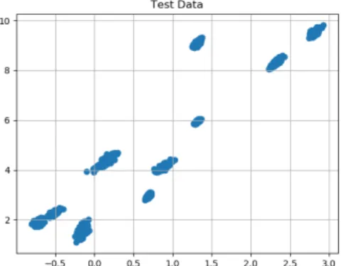
form of our model. However, in the simple form presented here, it is not as effective. In Figures 6-1 and 6-2 we can see how a model trained on Clustered Synthetic Data projects the train and test data in two dimensions. The obvious pattern is clusters that resemble lines. In contrast, we would like to see something that resembles tSNE’s output more.

Figure 6-1: Output of trained model on trained data. Output dimension is 2

Figure 6-2: Output of trained model on validation data.

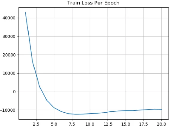
In addition, the solution obtained from this approach is unstable. As Figure 6-3 below shows, the KL divergence loss oscillates back and forth during the first 20 epochs. This problem is solved in the solution we presented in the Results Chapter of the report.

Finally, in Table 6.1 we can see the correctly predicted neighbors in the reduced test space. There are less points that were correctly compared to those numbers found in other approaches.

1 5 10 20

ℒKL 5 (0.5%) 51 (5.1%) 125 (12.5%) 216 (21.6%)

Table 6.1: Nearest Neighbors for the out-of-sample test. Test size is 1, 000.

6.3 KL Divergence Loss With Regularization

For the next approach, we decided to combine the first two ideas. Optimizing for the KL-divergence seems to be on the right track, so we added the sum of squared

(60)

error as a regularization term, in order to force the output similarities to resemble the input similarities even more.

Then, the objective becomes

ℒKL-SSE(𝑦1, 𝑦2, . . . , 𝑦𝑛; 𝑥1, 𝑥2, . . . , 𝑥𝑛) = ∑︁ 𝑖,𝑗 𝑝𝑖𝑗log (︁𝑝_𝑖𝑗 𝑞𝑖𝑗 )︁ + 𝜆∑︁ 𝑖,𝑗 (𝑝𝑖𝑗 − 𝑞𝑖𝑗)2

The addition of the regularization factor makes a clear difference on the outcome of the model. Before, the input and output space were mapped to clusters that resembled lines. In Figures 6-4 and 6-5 we can see that the clusters now have the form of clouds and are clearly separated from each other. One reason for why this happens might be that the sum of squared errors has a local minimum when 𝑦𝑖 = 𝑦𝑗

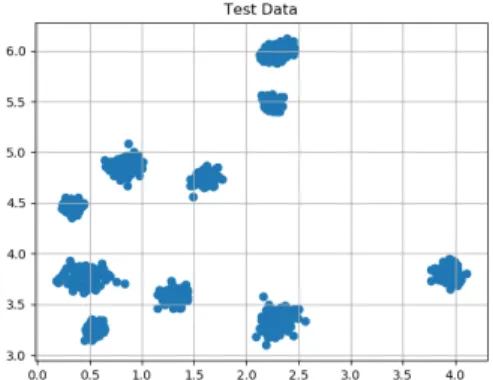
for all pairs (𝑖, 𝑗). In the extreme case of a very large regularization parameter 𝜆 the clusters collapse to points, so a reasonable value for 𝜆 produces the results below.

(61)

Observe that, in both this and the previous approaches the predicted test points appear exactly in the regions of the clusters of the reduced train space. This is a good indication that the model learns something valuable for the dataset.

Figure 6-4: Output of trained model on trained data. Output dimension is 2

Figure 6-5: Output of trained model on validation data.

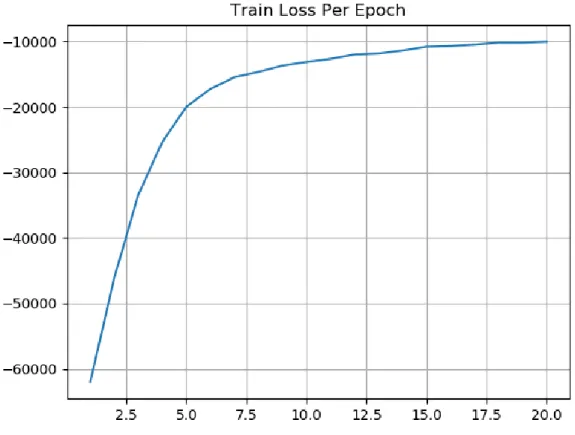
However, as happened in the KL divergence case, the loss function does not seem to stabilize while training. In Figure 6-6 we can see the loss in the training set per epoch of training. Even after 20 epochs, the loss oscillates up and down. This is an indication that the effect of the KL divergence factor is much larger than the effect of the regularization factor.

Finally, in Table 6.2 we can find the number of correctly predicted neighbors in the out-of-sample test. The numbers are clearly better than the numbers obtained with KL divergence alone. This fact is one more evidence that the addition of the sum of squared errors in the loss function improves the performance of the model.

1 5 10 20

ℒKL-SSE 11 (1.1%) 79 (7.9%) 187 (18.7%) 250 (25%)

Table 6.2: Nearest Neighbors for the out-of-sample test. Test size is 1, 000.

6.4 Discounted KL Divergence Loss

The last approach we tried was discounting the loss for pairs of points that are far from each other. The idea here is that we don’t care much about preserving the long

(62)

distances, so we might be better of by using the following loss function

ℒDISC(𝑦1, 𝑦2, . . . , 𝑦𝑛; 𝑥1, 𝑥2, . . . , 𝑥𝑛) = ∑︁ 𝑖,𝑗 𝑐𝑖𝑗𝑝𝑖𝑗log (︁𝑝_𝑖𝑗 𝑞𝑖𝑗 )︁ + 𝜆∑︁ 𝑖,𝑗 𝑐𝑖𝑗(𝑝𝑖𝑗 − 𝑞𝑖𝑗)2,

where 𝑐𝑖𝑗 = 1 if the distance between 𝑥𝑖 and 𝑥𝑗 is “small" and 𝑐𝑖𝑗 = 0.5. “Small" can

mean a lot of different things. For simplicity, we consider a distance 𝑑(𝑥𝑖, 𝑥𝑗) “small"

if point 𝑥𝑗 is one of the 20 points closest to 𝑥𝑖. Thus, the loss function weighs a lot

the top 20 points closest to some target points, and less the rest. This is true for any target points.

In order to achieve this, we store the 20 closest neighbors of every point as the model trains. The problem with this approach is that, while training the model, we cannot know whether a distance is small or large, until the model has seen a lot of pairs. Then, there are two disadvantages. First, all of the distances encountered in

A dimension reduction technique to preserve nearest neighbors on high dimensional data

A Dimension Reduction Technique to Preserve

Nearest Neighbors on High Dimensional Data

by

Christos Nestor Chachamis

B.S., Massachusetts Institute of Technology (2019)

Submitted to the Department of Electrical Engineering and Computer

Science

in partial fulfillment of the requirements for the degree of

Master of Engineering in Electrical Engineering and Computer Science

at the

MASSACHUSETTS INSTITUTE OF TECHNOLOGY

May 2020

c

○ Massachusetts Institute of Technology 2020. All rights reserved.

Author . . . .

Department of Electrical Engineering and Computer Science

May 18, 2020

Certified by . . . .

Samuel Madden

Professor

Thesis Supervisor

Accepted by . . . .

Katrina LaCurts

Chair, Master of Engineering Thesis Committee

A Dimension Reduction Technique to Preserve Nearest

Neighbors on High Dimensional Data

by

Christos Nestor Chachamis

Abstract

Acknowledgments

Contents

Chapter 1

Introduction

1.1

Introduction

1.2

Background and Related Work

1.2.1

ANN Search Methods

1.2.2

Dimension Reduction Techniques

Chapter 2

Model

2.1

General Model

2.2

Distance and Similarity

2.3

Loss Function

2.4

Training

2.5

Parameters

2.6

Model Variations

Chapter 3

Data

3.1

Clustered Synthetic Data

3.2

Large Clustered Synthetic Data

3.3

Clustered Synthetic Data with Noise

3.4

Uniform Synthetic Data

3.5

Real Data

Chapter 4

Methods and Metrics

4.1

Qualitative Features

4.2

Correctness

4.2.1

Out-of-sample Reduced Dataset Tests

4.2.2

Query Test

4.3

Efficiency