Programmable 2D Arrangements for Element Texture Design

HAL Id: hal-01520258

https://hal.inria.fr/hal-01520258

Submitted on 10 May 2017

HAL is a multi-disciplinary open access

archive for the deposit and dissemination of

sci-entific research documents, whether they are

pub-lished or not. The documents may come from

teaching and research institutions in France or

abroad, or from public or private research centers.

L’archive ouverte pluridisciplinaire HAL, est

destinée au dépôt et à la diffusion de documents

scientifiques de niveau recherche, publiés ou non,

émanant des établissements d’enseignement et de

recherche français ou étrangers, des laboratoires

publics ou privés.

Programmable 2D Arrangements for Element Texture

Design

Hugo Loi, Thomas Hurtut, Romain Vergne, Joëlle Thollot

To cite this version:

Hugo Loi, Thomas Hurtut, Romain Vergne, Joëlle Thollot. Programmable 2D Arrangements for

Element Texture Design. ACM Transactions on Graphics, Association for Computing Machinery,

2017, 36 (3), pp.Article No. 27 �10.1145/2983617�. �hal-01520258�

Programmable 2D Arrangements for Element Texture Design

ROMAIN VERGNE and JOELLE THOLLOT Inria-LJK (UGA, CNRS)

This paper introduces a programmable method for designing stationary 2D arrangements for element textures, namely textures made of small geo-metric elements. These textures are ubiquitous in numerous applications of computer-aided illustration. Previous methods, whether they be example-based or layout-example-based, lack control and can produce a limited range of pos-sible arrangements. Our approach targets technical artists who will design an arrangement by writing a script. These scripts are using three types of operators: partitioning operators for defining the broad-scale organization of the arrangement, mapping operators for controlling the local organiza-tion of elements, and merging operators for mixing different arrangements. These operators are designed so as to guarantee a stationary result mean-ing that the produced arrangements will always be repetitive. We show that this simple set of operators is sufficient to reach a much broader variety of arrangements than previous methods. Editing the script leads to predictable changes in the synthesized arrangement, which allows an easy iterative de-sign of complex structures. Finally, our operator set is extensible and can be adapted to application-dependent needs.

Categories and Subject Descriptors: I.3.7 [Computer Graphics]: cate-gory—Texture Synthesis; I.3.5 [Computer Graphics]: category—Artistic Rendering

General Terms: Algorithm

Additional Key Words and Phrases: Programmable approach, element tex-ture, spatial arrangement, texture design, texture synthesis

1. INTRODUCTION

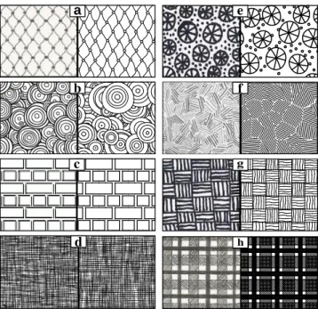
This paper introduces a programmable method for designing repet-itive arrangements of geometric elements. The design of such ar-rangements is a key component of element textures design in that it describes the geometric content of the texture. Element textures are a fundamental aspect of illustration (see Figure 1). They add complexity to a drawing and support many artistic effects. They also depict important information such as materials in architec-tural plans, fabric in clothes, terrain type in topographic maps, bi-ological materials in medical illustrations, etc. Producing element textures is therefore mandatory for many illustration systems and application fields, such as 2D animation, cartography, and other computer-assisted design tasks like pattern creation for textile or wallpaper industry. These applications often need to synthesize a large amount of each element texture either because the target im-age is very large (geographic map, wallpaper) or because the same texture is used in many images (comics, 2D animation). In this con-text, manual authoring quickly becomes tedious which motivates the need for a completely automated production pipeline. Several

a

e

b

f

c

d

Fig. 1. Element textures commonly used. Distributions with (a) con-tact, (b) overlap and (c) no adjacency between elements. (d) Over-lap of two textures creating cross hatching. (e) Non overOver-lapping com-bination of two textures. (f,g,h) Complex element textures with clus-ters of elements. For each example, we show a hand-drawn image (left), and our synthesized reproduction of its geometric arrangement (right). — Image credit: these textures can be found in professional art (d,g,h) [Guptill 1997], casual art (a,e,f) [profusionart.blogspot.com, hayesartclasses.blogspot.com], technical productions such as Computer-Assisted Design illustration tools (c) [www.compugraphx.com], and textile industry (b) [www.123stitch.com].

problems need to be solved to achieve this goal: the synthesis of various geometric elements, their arrangement on the plane, the choice of style attributes for each element and the rendering of the final element texture. Each of these topics is a research problem in itself. Existing works address extensively the tasks of creating ele-ments [Baxter and Anjyo 2006; Hurtut and Landes 2012; Campbell and Kautz 2014] as well as stylizing and rendering geometrical data [Hertzmann 2002; Eisemann et al. 2008; Grabli et al. 2010; DiVerdi 2013]. In this article we address the problem of spatiallyarranging existing elements so as to fill a given region. We do not restrict our approach to tielable arrangements but instead we provide a way to

fill regions of any size or shape with arrangements that may contain tiled repetitions, depending on the designer’s intent.

Targeted Properties. A computer-aided design tool for the pro-duction of arrangements should meet several requirements which we formalize in the following targeted properties:

—Predictability. Iterations between clients and technical artists in-volve numerous edits of the produced arrangements, which is feasible only through a controllable synthesis engine with pre-dictable results.

—Expressiveness. The design tool must be expressive enough to al-low the creation of classic layouts used by technical artists (see Figure 1 for an overview). When looking at manually drawn pat-terns, we observe that artists use regular and non-regular ele-ments distributions and control eleele-ments’ adjacency such as con-tact or overlap. Complex arrangements are obtained by compos-ing multiple distributions, the composition rule becompos-ing generally a non-overlap superposition of these distributions. Some arrange-ments are also structured into clusters of elearrange-ments and can be thought of as being based on multi-scale arrangements. —Usability. Experienced users should be able to quickly and

eas-ily design or edit arrangements. A canonical and intuitive set of operations should also be provided to ensure a gentle learning curve of the design tool.

—Extensibility. Some specific projects might need arrangements that cannot be initially produced by the design tool, despite its native expressiveness. It must then provide a way to add new components for synthesizing these arrangements, while still guaranteeing the above properties.

Our Approach. We propose a programming-based method where each arrangement is represented by a user-written script. Pro-grammable approaches have been proven useful for many design-ing tasks in computer graphics, includdesign-ing shaddesign-ing [Cook 1984], modeling [Müller et al. 2006], stylized rendering of 3D scenes [Grabli et al. 2010; Eisemann et al. 2008] and motion effects [Schmid et al. 2010]. As in these works, we target artists hav-ing programmhav-ing abilities such as technical directors. Textures are specific since they are repetitive, enforcing their perception as a whole [Treisman and Gelade 1980]. This characteristic can be for-malized as the result of a stationary process, meaning that the spatial statistics of an arrangement should not depend on its spa-tial location. Our contribution is therefore to provide the first pro-grammable design tool dedicated to the creation of stationary ar-rangements while satisfying the four properties defined above.

Technical Contribution. To build our programmable method, we define a set of predictable operators that allow to produce a wide va-riety of arrangements while ensuring their stationarity. For that we take inspiration from programmable raster texture design1_{. In these} methods, the design process (1) starts with an initialization such as Perlin’s noise, (2) involves a number of filters such as color map-ping, and (3) uses combining operations such as blending to mix multiple textures. Instead of a pixel grid, we store our arrangements in a high-level structure that stores adjacency and geometric infor-mation. Then, similarly to raster texture, we introduce three types of operations for the design process: (1) the structure is initialized with stationary partitions such as a grid; (2) instead of filters, lo-cal geometric transformations are next applied to refine the parti-tions; (3) merging operators finally allow multiple arrangements to

1_{www.allegorithmic.com}

be combined into complex ones. These three categories of operators are sufficient to achieve expressiveness, while creating a modeling scheme where stationarity is guaranteed at all stages. The synthe-sis is controlled step-by-step, which allows to edit the script with predictable effects. Finally, our method can easily be extended by adding new operators as long as they satisfy the conditions that pre-serve stationarity.

2. RELATED WORK

We focus our study on object-based texture representations, such as vector graphics representations, rather than their raster coun-terpart. Indeed, even if some efficient methods have been devised in the context of raster textures design [Ebert et al. 2002], pixel-based textures lose geometric and connectivity information of the elements at stake, preventing further stylization or editing. In the context of object-based texture representation, existing computer-aided solutions for element placement fall into two main categories: example-based approaches which have seen a recent increased in-terest, and layout-based solutions usually proposed in commer-cial software. After reviewing these two classes of approaches that allow to produce stationary arrangements, we will review other procedural modeling approaches that are more expressive or pre-dictable but lose stationarity.

2.1 Example-Based Element Texture Synthesis

Most methods in the literature of element textures synthesis are dedicated to example-based approaches. They propose an artist-friendly interface where a small user-drawn exemplar is analyzed and synthesized over a larger domain. These approaches produce stationary arrangements and are easy to use for casual users. How-ever they have a limited use in industrial contexts due to their lack of predictability and expressiveness.

Predictability. Describing the texture through a single exemplar brings an ambiguity between desired invariants (such as “all ele-ments must touch each other at their ends”) and variable proper-ties (such as “elements can have random orientations”). Further-more, small modifications in the exemplar may produce large un-predictable changes in the output. Besides, the exemplar needs to be stationary. So any modification has to be spread all over the ex-emplar meaning that the user has to rearrange the entire exex-emplar at each design iteration.

Expressiveness. None of the existing example-based methods succeeds to cover all classic layouts presented in Figure 1. We tested four recent methods [Ijiri et al. 2008; Hurtut et al. 2009; Ma et al. 2011; Landes et al. 2013] and we observed limitations con-trolling contact or overlap (Figure 2(a)), regularities such as align-ments (Figures 2(b) and 2(c)) and multi-level arrangealign-ments (Figure 2(d)). These limitations come from two fundamental issues. First, approximate representations limit the types of elements and ad-jacencies that can be handled. For example, a centroidal element model [Ijiri et al. 2008] is not adapted to strongly anisotropic el-ements. The perceptually-based approach of [Barla et al. 2006] is also limited to the synthesis of simple strokes and irregular pat-terns. Similarly, bounding boxes [Hurtut et al. 2009] or sampling [Ma et al. 2011; Xing et al. 2014; Roveri et al. 2015] reduce con-trol on adjacency (Figure 2(a)). The proxy geometries introduced in [Landes et al. 2013] help to control more precisely elements ad-jacency. However, it does not solve overlapping cases due to an inaccurate similarity measure of overlapping relations. Second, the lack of high-level information makes it hard to detect geometrical

[Ijiri et al., 2008] [Hurtut et al., 2009] [Ma et al,. 2011]

(a)

(b)

(c)

(d)

[Landes et al,. 2013] Our approach

Fig. 2. Example-based methods’ limitations. Input exemplars are shown on the left. Synthesized results from previous methods [Ijiri et al. 2008; Hurtut et al. 2009; Ma et al. 2011; Landes et al. 2013] are shown on the next four columns. Our results are shown on the last column.(a) A bimodal hatching, explicitly cited as one of the last limitations in [Hurtut et al. 2009]. While each interior hatch drawn in the exemplar crosses exactly three other hatches, no method preserves this property.(b,c) Regular structures with respect to three and one axis of alignment. Dense packing is challenging for Monte-Carlo statistical approaches [Hurtut et al. 2009; Landes et al. 2013] while growing approaches tend to create some gaps [Ijiri et al. 2008].(d) A simple case of element clusters that no method succeeds to reproduce faithfully. With our approach, we go beyond by-example methods’ limitations by faithfully reproducing the target arrangements with an appropriate set of operators. Note that we only handle the geometry of the underlying texture. The stylization step can be done afterwards, using any vector graphics software.

constraints at variable scales such as alignments and clusters. Re-cent by-example techniques [AlMeraj et al. 2013a; Emilien et al. 2015] demonstrate improved results, but cannot handle structured textures. It has been done for specific applications, like in [Yeh et al. 2013] for arrangements of tiles, but we are looking for a more gen-eral approach.

2.2 Predefined Layouts

Vector graphics software such as Adobe Illustrator or Inkscape pro-pose predefined layouts to arrange user-drawn elements. The most common example of such layouts is the grid. With the same ap-proach, recent online tools2_{propose methods for tiling small} user-drawn arrangements. More complex stand-alone algorithms can synthesize uniform distributions efficiently [Hiller et al. 2003; La-gae and Dutré 2005]. All these methods produce stationary results and are straightforward to use for obtaining a single particular lay-out. Their effect is predictable but their expressiveness is limited to a single kind of arrangement and they are usually not easily ex-tendable. Typically Figure 2(d) would be hard to do with such ap-proaches because it mixes regular and random distributions.

2_{www.colourlovers.com/seamless}

2.3 Procedural Modeling

In this section, we first present several inspiring procedural meth-ods coming from fields other than texture synthesis. Historically, L-Systems [Lindenmayer 1968] were used early in computer graph-ics to model plants [Prusinkiewicz and Lindenmayer 1996]. Being originally dedicated to the generation of one-dimensional patterns, they cannot enforce a stationarity property in a two-dimensional domain. This is also the case for their extensions: parametric, timed and open L-Systems.

Shape grammars are another renowned procedural modeling ap-proach [Stiny et al. 1971; Wonka et al. 2003; Müller et al. 2006]. Like more general context-dependent growth systems [Wong et al. 1998; Mˇech and Miller 2012], they use an axiom that is either a single element or the domain boundary. User-programmed growth rules must handle the propagation (or the subdivision) into the en-tire domain. Consequently, users would have to make a careful, non-intuitive use of each rule to obtain stationary arrangements.

Other arrangement transformations have been studied such as parquet deformations [Kaplan 2010] and Escher construction oper-ators [Henderson 2002]. These models are specific to their respec-tive application fields, which limits their expressiveness. However they are similar to our approach in the sense that they locally ap-ply geometric transformations to an initial partition. Our approach targets general stationary arrangements.

Recently, a first grammar-based approach has been proposed for the procedural generation of specific repetitive simple patterns called zentangles [Santoni and Pellacini 2016]. These pen-and-ink patterns are highly recursive in their structure and based on a small set of geometric shapes. Based on a grammar model, using group-ing and splittgroup-ing operators, this method allows the concise design of zentangles. The authors compare their approach to ours in their paper. Due to the grammar-based approach, this approach is a little less expressive and less easily extensible than our programmable approach.

3. DATA STRUCTURE

We represent our arrangements of geometric elements as a collec-tion of curves embedded into a planar map: a topological modeling tool introduced in [Baudelaire and Gangnet 1989] for represent-ing drawrepresent-ings. This structure contains vertices (intersection points), edges (pieces of curves linking vertices) and faces (2D domains enclosed by edges). Spatial adjacency between these three types of cells can be easily handled, providing an easy access to precise topological relations between them such as intersections, contacts, and inclusions.

Definition. The planar map induced from a collection of curves Cis defined as a set of cells partitioning the plane (Figure 4). Cells are of three types: edges, vertices and faces. Edges are the set of maximal pairwise disjoint subcurves of C. Vertices are the set of limit end points of edges. Faces are the set of maximal parts of R2´ C. An incidence graph completes the representation allowing access to all types of adjacencies in the planar map.

Cell labels. On top of the planar map, we add a set of labels to each cell. They will typically be used to select a subset of cells when needed and are set by the user at the initialization step.

Face labels reconstruction.When modifying or combining pla-nar maps, labelling has to be conserved. We adopt the same solution as [Asente et al. 2007]. Since planar maps are induced by curves, labels should be stored only on curves. Faces labels are thus stored on their adjacent edges and reconstructed each time a new planar map is induced.

Implementation.Practically, in our implementation, planar maps are based on the CGAL arrangement structure [Fogel et al. 2012] and use exact arithmetic and geometry with rational coordinates to avoid any topological artifacts due to numerical imprecision.

4. OVERVIEW

Design principles. In a programmable approach, the task of the user is to build the algorithm that will produce his envisioned result. For that we provide the user with three types of operators, each of them responsible of a specific task: partitioning operators initialize an ar-rangement, mapping operators refine it and merging operators cre-ate combinations of arrangements. All of these operators have to guarantee the stationarity of the resulting arrangement. The texton theory [Julesz 1981] states that the appearance of an arrangement emerges from the broad-scale organization of micro-patterns called “local texture elements”. Therefore stationarity occurs at broad-scale whereas local texture elements do not need to be constrained. Following this theory each type of operator will guarantee station-arity at its own scale:

—Partitioning operators. The design of an arrangement starts with a stationary partition. It ensures stationarity at broad-scale while letting the user choose between a regular or non-regular global arrangement structure.

—Mappers. The initial partition is locally refined using mappers. Mappers are user-programmed functors and control both local geometry and adjacency, for instance by placing an imported el-ement and transforming it depending on its neighbors. A mapper is always applied everywhere on the arrangement via a mapping operator. Whereas no specific property has to be satisfied by el-ements, this is the locality and the homogeneous application of the mapper all over the arrangement that will ensure stationarity. Note that mappers can also call a partitioning operator in order to create a subscale arrangement. This can be useful to create tex-ture elements made of stationary arrangements (see for instance the subscale stripe arrangements in Figure 1(g)).

—Merging operators. Finally, complex arrangements are some-times more easily designed when seen as the merge of simple arrangements such as the overlap of two textures. Merging oper-atorsprovide such mechanisms by performing overlap, inclusion and exclusion operations. They do not change the stationarity of their input arrangements.

Functional programming. Our approach is entirely functional. We define an arrangement as a function that takes as input a re-gion and returns a collection of curves. All our operators, regard-less of their category (partitioning, mapping, merging), output an arrangement. On the input side, partitioning operators take in a re-gion whereas merging operators take in two arrangements to be combined. Mapping operators take in both a mapper and an ar-rangement to be mapped. We use Python as the programming user interface, its syntax being simple and intuitive to most program-mers and well designed for functional programming.

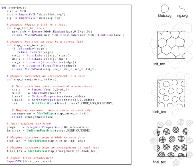
Overview example. Figure 3 gives an example of the synthesis of a two-scale arrangement. Three mappers are first designed in this script. The first two ones map an SVG element on a face (L.9) and an edge (L.19). The last one creates a regular partition (L.29) and calls the second mapper (L.32) to map a curve on each of its edges. Once these mappers are defined, a uniform partition is cre-ated (L.37). A blob shape is mapped on each of its faces using the first mapper (L.40). The third mapper then maps a regular arrange-ment on the resulting faces which are now blobs (L.43). Induced edges and faces are exported respectively as open and closed SVG polylines (L.46).

5. PARTITIONING OPERATORS

The first step in the design of an arrangement is to choose a partition to define its global structure. Such partitions must be stationary and should hold a regular or non-regular global structure. These parti-tions will be extensively refined by defining local transformaparti-tions using mappers, as presented in Section 6. If required, more opera-tors could be easily added to adapt to specific needs. Our goal in this section is therefore to provide operators that ensure a station-ary partition, simple enough to begin the design, but subsequently flexible enough to allow all possible refinements.

We propose four partitioning operators that allow to design reg-ular and non-regreg-ular partitions of the input region. These operators, in addition to a few others that let specify partition labels and prop-erties, are recalled in the Table II of the appendix.

1 d e f overview ( ) : 2 s i z e = 2000 3 b l o b = ImportSVG( " d a t a / b l o b . svg " ) 4 z i g = ImportSVG( " d a t a / z i g . svg " ) 5 6 # Mapper : P l a c e s a b l o b i n a f a c e . 7 d e f map_blob_to ( f a c e ) :

8 new_blob = R o t a t e( blob ,Random( f a c e , 0 , 2 ∗ pi , 0 ) )

9 r e t u r n M a t c h P o i n t( new_blob ,BBoxCenter( new_blob ) ,C e n t r o i d( f a c e ) )

10 11 # Mapper : R e p l a c e s an e d g e by a c u r v e d l i n e . 12 d e f map_curve_to ( edge ) : 13 i f I s B o u n d a r y( edge ) : 14 r e t u r n ToCurve( edge ) 15 s r c _ c = P o i n t L a b e l e d( zig , " s t a r t " ) 16 d s t _ c = P o i n t L a b e l e d( zig , " end " ) 17 s r c _ v = L o c a t i o n(S o u r c e V e r t e x( edge ) ) 18 d s t _ v = L o c a t i o n(T a r g e t V e r t e x( edge ) ) 19 r e t u r n M a t c h P o i n t s( zig , s r c _ c , d s t _ c , src_v , d s t _ v ) 20 21 # Mapper : G e n e r a t e s an a r r a n g e m e n t i n a f a c e . 22 d e f m a p _ a r r a n g e m e n t _ t o ( f a c e ) : 23 24 # G r i d p a r t i t i o n w i t h r a n d o m i z e d o r i e n t a t i o n s 25 t h e t a = Random( f a c e , 0 , 2 ∗ pi , 1 ) 26 wi dth = BBoxWidth( f a c e ) / 5 27 l i n e s 1 = S t r i p e s P r o p e r t i e s( t h e t a , wid th ) 28 l i n e s 2 = S t r i p e s P r o p e r t i e s( t h e t a + p i / 2 , wid th ) 29 i n i t = G r i d P a r t i t i o n( l i n e s 1 , l i n e s 2 ,CROP_ADD_BOUNDARY) 30 31 # Mapping o p e r a t o r : maps a c u r v e on e a c h e d g e 32 a r r a n g e m e n t = MapToEdges( map_curve_to , i n i t ) 33 r e t u r n a r r a n g e m e n t ( f a c e ) 34 35 # I n i t : U n i f o r m p a r t i t i o n 36 p r o p s = I r r e g u l a r P r o p e r t i e s( 1 0 / ( s i z e ∗ s i z e ) )

37 i n i t _ t e x = UniformPartition( props , KEEP_OUTSIDE ) 38 39 # Mapping o p e r a t o r : maps a b l o b i n e a c h f a c e 40 b l o b _ t e x = MapToFaces( map_blob_to , i n i t _ t e x ) 41 42 # Mapping o p e r a t o r : maps an a r r a n g e m e n t i n e a c h f a c e 43 f i n a l _ t e x = MapToFaces( map_arrangement_to , b l o b _ t e x ) 44 45 # E x p o r t f i n a l a r r a n g e m e n t 46 ExportSVG( f i n a l _ t e x , s i z e ) init_tex blob.svg zig.svg blob_tex final_tex

Fig. 3. An example of a script and its output. Left: A script based on two imported SVG elements (a blob-like shape and a small stroke) and three user-defined local mappers to control local features.Right: The output is a two-scale arrangement. We show here two imported elements, followed by the two intermediary results and the final output. The square window represents the filled output region: Transparent lines are shown for clarity, yet they are not in the actual arrangement.

Three oriented curves Induced planar map Incidence graph

Fig. 4. Planar map representation. Left: Three oriented curves. Middle: Induced planar map composed of nine vertices, nine edges and two faces. The face f0is unbounded. Edges are oriented accordingly to their origi-nating curves. For example, e1’s source vertex is v2and its target vertex is v3.Right: The incidence graph of the planar map denotes the relationships between vertices, edges and faces. We did not include arcs between vertices and faces for clarity, they can be deduced by transitivity.

Regular partitions. The “StripesPartition” operator partitions the domain with a distribution of parallel lines. This operator is de-fined with the stripe angle and the width between two successive lines. Optionally, the user may define a cycle of widths that will be repeated periodically until all lines are placed. For instance in Figure 5(a) the top image shows a cycle with two alternating width values (20 units and 10 units), while the bottom image uses only one width value (15 units). These parameters are set by the "StripesProperties" function that takes a variable number of argu-ments. Labels might also be associated to faces and/or edges using the same cycle process. In that case, all partition’s faces/edges are labelled by successively picking the corresponding value in the la-bel list (Figure 5(a)). “GridPartition” partitions the domain with two distributions of parallel lines and is thus obtained by specify-ing two stripes partitions. Note that when faces are labelled for both stripes, each single face receives a total of two labels. For instance in the top image of Figure 5(b), the green color denotes the pres-ence of both labels “yellow” and “blue”.

(a) Stripes (b) Grid (c) Uniform (d) Random Fig. 5. Available types of partition. When designing an arrangement, the first step is to choose a type of partition among four possible ones, whether it is a regular (a,b) or a non-regular partition (c,d). Colors denote assigned labels to faces (top) or edges (bottom). We vary the width between lines of regular partitions using periodic cycles of values. The same process is used to assign labels. The density of irregular partitions is controlled by a single parameter. Labels may also randomly be assigned according to user-defined probabilities. Faces and edges may contain multiple (cycling) labels to precisely control the final arrangement.

Non-regular partitions. “UniformPartition” and “RandomParti-tion” operators are computed using Voronoi diagrams, respectively based on Poisson-Disk and Poisson distributions. In both cases, the user needs to specify a density value that defines the number of samples per unit area via the "IrregularProperties" function. Labels might also be attached to faces and edges of these partitions. In that case, the user defines a list of probabilities used to randomly assign labels to faces and/or edges (Figure 5(c,d)).

(a) CROP (b) CROP_ADD_BOUNDARY

(c) KEEP_INSIDE (d) KEEP_OUTSIDE

Fig. 6. Border behaviors. The user can choose between four partition behaviors at the domain’s border. In these illustrations, a uniform partition is created on a light blue domain. One can first simply crop the partition along the border (a), with possibly adding the domain’s outline curve (b). The cells of the partition that overlap the border can also be discarded (c) or kept (d).

When partitioning a face, the user may want various behav-iors at its boundary. We provide four border management op-tions that cover all the cases we encountered (Figure 6). The CROP option cuts the partition at the boundary of the face. The

CROP_ADD_BOUNDARY option does the same except that it adds the outline curve of the face. For these two options, the re-sulting planar map usually ends up with faces with a different shape on the border than in the middle of the original face. If one prefers to keep constant face shapes, like to keep constant grid cells, he can choose between two other options: KEEP_INSIDE or KEEP_OUTSIDE. The first option keeps only the cells that are strictly included in the original face whereas the latter keeps all the cells that intersect the original face. The resulting cells can thus overlap the face border. Note that stripes partitions are always cropped as their faces are infinite.

6. MAPPERS

Mappers are a central feature of our approach. As previously men-tioned, a texture is a large-scale stationary arrangement of small-scaleelements. Contrary to partitioning operators that create the broad-scale structure of the arrangement, mappers are targeting small-scale elements. In practice, a mapper is a function that takes as input a single cell of a planar map. It applies (almost) arbitrary code written by the user so as to create, combine, transform and place curves on a particular location according to the cell’s infor-mation (position, incident vertices, edges, faces, etc.). Finally, a mapper outputs a collection of curves.

In order to preserve stationarity, mappers must be executed ho-mogeneously on all the cells of a planar map. Since the initial pla-nar map comes from a statiopla-nary partition, this property is pre-served, formalizing the large-scale repetitive aspect of textures. This homogeneous execution is handled by mapping operators. We provide one mapping operator per cell’s type: "MapToVertices", "MapToEdges" and "MapToFaces" (Table III in appendix). A map-ping operator takes as arguments the arrangement to be mapped and a user-programmed mapper. Its output is a new set of (stationary) curves. It is worth noting that the resulting arrangement can in turn be used as input to another mapping operator in order to generate more complex patterns.

6.1 Mapper Definition

Formally, a mapper is a user-programmed functor m that maps a single cell c of a planar map P to a new collection of curves C. The key idea of our model is that the programmed functor m will au-tomatically be executed on each cell c P P by a mapping operator. To ensure that the mapping of m on P preserves stationarity, the following conditions must be respected:

—m is local and depends only on cells of P inside a given bounded neighborhood. Only a bounded number of incidence queries should then be called inside a given functor.

—m does not depend on a particular execution order. It means that global variables are read-only and should not be overwritten. —m does not depend on global coordinates to avoid specific

map-pings to be applied at particular locations in the plane. Conse-quently, only relative cell’s coordinates are available from the user point of view.

These conditions ensure that a functor will have the same behavior everywhere in the input planar map.

6.2 Programming Mappers

We provide a set of low-level built-in operators specifically de-signed to program mappers, given in Table IV of the appendix. All the examples shown in this paper have been created with this sim-ple operator set:

—Incidence operators are dedicated to access all the information stored in the incidence graph of the planar map. For example, for an edge we give access to the two vertices creating this edge, to the two faces that are separated by this edge. And this is similar for all the cells types.

—Adjacency operators are used to place elements while controlling their adjacency either to one or two vertices, or in a face. It allows to precisely place an element in given cells of the planar map and is typically used to replace each edge by a user designed curve or to put an element centered and scaled in each face.

—Geometry operators retrieve information of the input cell such as its location, contour, centroid, etc.

—Label operators are dedicated to the management of labels. —Random values operators allow to easily vary the properties of

the mapping inside each cell.

We also provide a set of useful utility functions that yield simple geometric affine transformations, bounding box information as well as the loading of an SVG element. These functions are accessible from everywhere in user-scripts (see Table VI of the appendix).

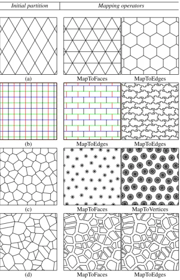
Initial partition Mapping operators

(a) MapToFaces MapToEdges

(b) MapToEdges MapToEdges

(c) MapToFaces MapToVertices

(d) MapToFaces MapToEdges

Fig. 7. Using mappers. Four examples of mappers effect on initialized partitions.

6.3 Using Mappers

A typical use of mapping operators is to modify an original parti-tion, for instance by removing or modifying some cells, then plac-ing some new elements possibly controllplac-ing their adjacency. One can stop here or continue to map elements until reaching the de-sired arrangement. We show four examples in Figure 7 to illustrate the variety of effects a mapper allows to create on the partitions: —(a) A grid is first initialized using the "GridPartition" operator

(left). A line is then inserted inside each face to obtain a sub-divided triangular arrangement (middle). The hexagonal parti-tion (right) is obtained by replacing edges by their duals: lines connecting the centroids of adjacent faces. These two partitions could themselves be used as starting points for other mappers. —(b) Each edge of an initial grid partition (left) is labelled using

user-defined value cycles (shown with colors in this example). Based on the "HasLabel" operator, a mapper that keeps edges in staggered rows is applied on each edge of the grid (middle). The final puzzle pattern is obtained by a mapper using the "Match-Points" operator that places a simple curved line on each edge (right).

—(c) The planar map is initialized with a uniform partition (left). Four lines are matched to the centroid of each face of the parti-tion to build a new set of construcparti-tion lines (middle). Overlap-ping circles are mapped on the resulting vertices to create rosette flowers (right).

—(d) Starting from a random initial partition (left), the induced faces are slightly scaled down (middle). Some curves, picked from a limited example set are finally mapped on each induced edge using the "MatchPoints" operator (right).

More complex arrangements can be created by calling partitions operators into mappers as shown in the overview (Figure 3).

7. MERGING OPERATORS

Merging operatorstake two arrangements as inputs, and return one arrangement (Figure 8). They provide a simple way to mix simple arrangements to obtain complex patterns. We propose three differ-ent merging operators (Table V):

—Union computes a new arrangement that results from the collec-tion of all the edges produced by the two inputs arrangements. It is used to group multiple distributions (Figure 8(d)).

—Inside and Outside are masking operators. They keep only the edges produced by a first arrangement that are falling inside and outside the bounded faces, respectively, of a second arrangement. A border management option is mandatory for these operators. It allows to precisely define if cells have to be kept-in, kept-out or cropped along the first arrangement boundaries (Figure 8(e-h)).

8. RESULTS

Along the paper we have shown that our method guarantees station-ary outputs by construction. We also have highlighted how it is ex-tensible at all stages. Here we present practical modeling sessions that demonstrate its predictability and expressiveness. Designing an arrangement is an iterative process. The user progressively finds the set of successive rules that leads to the result he has in mind. As shown along the paper, the basic strategy is to design simple ar-rangements to be combined. A general structure is chosen for each one, and further refined. All the scripts and execution times used

(a) tex1 (b) tex2

(c) tex3 (d) Union(tex1,tex2)

(e) Inside(tex2,tex1,CROP) (f) Inside(tex3,tex1,KEEP_OUTSIDE)

(g) Outside(tex3,tex1,CROP) (h) Outside(tex3,tex1,KEEP_INSIDE) Fig. 8. Merging multiple distributions. (a,b,c) Three simple arrange-ments obtained via partitioning and mapping operators.(d) The Union oper-ator overlaps its two input arrangements.(e,f) The Inside operator behaves like a mask, keeping only the edges from a first arrangement that fall in-side the faces of a second one. The same border management options are proposed as for partitions (see Figure 6).(g,h) The Outside operator also behaves like a mask, keeping only the edges from a first arrangement that fall outside the faces of a second one. Same border management options are available.

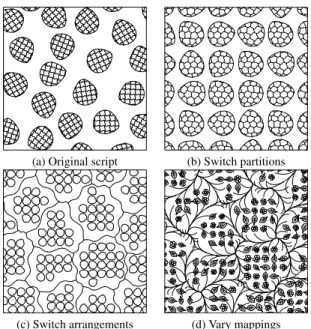
(a) Original script (b) Switch partitions

(c) Switch arrangements (d) Vary mappings

Fig. 9. Script edition. A design strategy can be to edit iteratively a starting arrangement.(a) Original two-scale arrangement from Figure 3. (b) The grid partition previously applied to the lower scale is exchanged with the uniform partition from the blob distribution.(c) Another inversion: blobs are now regularly distributed inside the uniformly distributed cells.(d) A twig is mapped to the smooth stroke of (c), and flowers or leafs with varying scales are now mapped to the blob shape.

Fig. 10. Comparison with exemplar-based approaches. The evaluation protocol developed in [AlMeraj et al. 2013b] showed that even expert de-signers do not usually agree on what should be the output arrangement based on one exemplar. We show here that we can reproduce the four different expert manual arrangements gathered in the second figure from AlMeraj’s study, which all subtly vary from the given input exemplar. to produce the images of this paper are included in the supplemen-tal materials. Most results were generated in a few seconds (except Figures 1(b,d) and 12(d) that needed more than one minute).

(a)

Grid Rotate faces Scale faces Stripes Outside

(b)

Grid Remove Edges Scale faces Map stripes

(c)

Stripes Map curve Merge Map random rotated stripes

(d)

Grid Map circle Scale faces Delete random faces

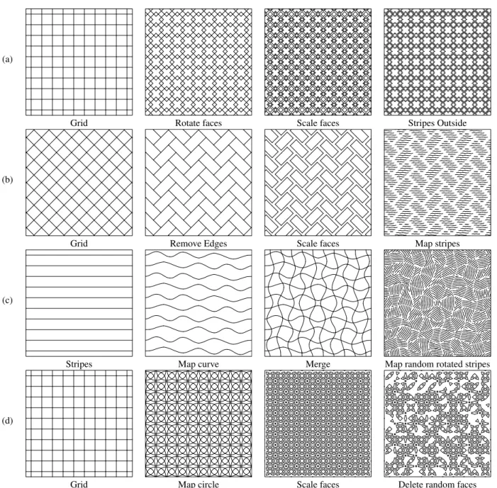
Fig. 11. Creating complex structures starting from regular partitions. Each row shows some iterative design steps, starting from an initial regular partition.(a,b,c) Two-scale examples where the initial partition is refined in different ways, and the resulting regions filled with various stripe patterns to produce hatching effects.(d) A mosaic-like partition is made using a grid and mapped circles. A kind of aging effect is finally obtained by deleting some faces randomly.

Script Editing. In terms of interaction, our modeling approach is very similar to node-based material shaders commonly used in the 3D pipeline: (1) partitioning operators correspond to initialization nodes, (2) mapping operators correspond to filtering nodes, and (3) merging operators correspond to the 2 Ñ 1 combination nodes. This interaction scheme has been used during the last 30 years since the seminal work on Shade Trees [Cook 1984]. It is commonly ac-knowledged to be efficient. In particular, it favors iterative design processes as well as the exploration of various combinations at the artist’s whim.

Figure 9 shows the kind of variations that are produced during such an exploratory usage of our tool. Each image shows the re-sult obtained by a slight modification of the script presented in the overview (Figure 3). These variations are predictable because the script is composed of small understandable chunks of code (parti-tions and mappers) linked together by simple merging operators. A regular user of our tool should be able to foresee how these edits in the script will influence the execution of the other chunks left unchanged.

In Figures 11 and 12 we show iterative design sessions where the user envisions a particular arrangement and edits the result

to-(a)

Uniform Map circle Uniform Map curve and scale faces

(b)

Random Map curve Map Random Map curve

(c)

Uniform 1 Scale faces Uniform scaled 2 2 Inside 1

(d)

Random Scale edges x5 Scale edges x10 Rotate edges

Fig. 12. Creating complex structures starting from non regular partitions. (a) First row shows two examples starting from a uniform partition, yet with radically different final arrangements.(b) A random partition, after having mapped its edges with a curve, is recursively applied to its own regions, achieving a two-scale cracks effect.(c) Another two-scale arrangement, based on an inside merging operator, leading to a turtle shell effect. (d) The arrangements can quickly depart from the initial partition, even with simple refinements: the edges of a random partition are directly scaled then rotated to produce various random lines distributions.

wards this objective. Our method allows to proceed step by step and to display the arrangements produced at each step. This helps making sure that the edits converge towards the envisioned result. These two figures display the temporary steps of the design ses-sions as well as the results finally obtained. They showcase how this script-editing scheme is helpful for quickly designing complex arrangements.

All the scripts producing these examples have less than 60 human-readable lines and they use only the operators given in ap-pendix.

Expressiveness. All the examples shown in this section demon-strate that the arrangement properties we mentionned in Section 1 can be obtained with our set of operators: regular and non-regular arrangements, various elements adjacency relations such as contact or overlap, compositions of several arrangements and clusters of elements. Figures 2 and 10 show that our approach overcomes the limitations of existing example-based techniques. In Figure 13, we show how multi-level partitions can interact together (top) and how labels can be used to create some interactions between arrange-ments allowing to create complex structures in a controllable way.

(a) (b) (c)

Fig. 13. Interactions between arrangements’ scales. Top: a random partition (a) is used as a basis to distribute regularly spaced squares (b). A curve is placed inside each square oriented around the center of the initial partition in(c). Bottom: this CPU-like arrangement is composed of two levels: chips and junctions connected together.(a) Junctions are created using SVG elements mapped on an initial random partition. (b) Chips are created using the same method and each chip is labelled.(c) These two arrangements are merged using the Outside operator and a mapper uses the labeling information to generate two kinds of connectors depending on the vertices status (end points and chip junctions).

These results demonstrate that expressiveness is achievable with a restrained set of operators. It also validates our insight of sep-arating the design tasks between a very small set of partitioning operators and an unlimited set of possible refinements. It is partic-ularly visible in Figure 11 where a variety of arrangements are de-signed based on simplistic regular partitions. Figure 14 also shows that more complex tilings can be easily created such as wallpaper groups tilings.

These results validate as well our choice of manipulating all kinds of primitives (vertices, edges and faces), whereas alternative strategies based only on dot anchors or edge distributions would limit the possible spectrum of edits.

Applications. Elements arrangements are usually not the final re-sult of an artistic production. We show here examples of applica-tions that make use of elements arrangements produced by our ap-proach to demonstrate the variety of possible applications of such data.

—3D Texturing. The interaction between light and surfaces in 3D scenes is most often described via materials, which represent the color of the surface, its albedo, roughness, etc. The variations of these parameters along the surface can be painted by artists as textures. For textures exhibiting geometrical repetitions, such as cracks in ice, painted ornaments on furniture, elements arrange-ment can easily be designed via our tool and then rasterized to include them in a 3D rendering pipeline as a texture layer. Fig-ure 15 shows examples of 3D scenes where element arrange-ments shown earlier in the paper guide the materials’ parameters. —3D Modeling. In many 3D scenes, objects themselves are ar-ranged repetitively on surfaces: trees on a forest ground, bricks

on a wall... These arrangements can also be synthesized effi-ciently using our method, and then converted to 3D meshes using extrusion, proxies (replacing each 2D element by a 3D mesh) or another procedural system (make a tree grow starting from each element). Figure 16(top) shows an example of mosaic extruded from a 2D arrangement synthesized using our method.

—Fabrication. Most of the objects being computer-fabricated to-day require fabrication instructions in the form of cutting paths or volumes to fill with a certain material. In both cases, the vec-tor representation of element arrangements can be leveraged so as to generate automatically a significant part of these instruc-tions. Figure 16(bottom) shows examples of laser-cut pieces of furnitures where over 95% of the cutting paths were generated using our system.

9. USER STUDY

We evaluated the practical use of our model by asking eight users to produce three arrangements as close as possible to three target examples we gave them. As detailed in the following, these users attended the same supervised tutorial session in order to get them familiar with our tool before working on their own in an unsuper-vised session. The tutorial, the script files and rendered arrange-ments are all available as supplemental materials.

9.1 Procedure

In order to obtain comparable results, the user-study has been con-ducted under the following procedure:

—All participants have backgrounds similar to technical directors. They have either a master degree in Computer Science or a

ti-Fig. 14. Creating wallpaper groups tilings of the plane. (Top) An arrangement with symmetry group P6 (left) is obtained from an hexagonal tiling (Figure 7(a, right)) followed by a mapper replacing each edge with a “Z”-shaped curve. An arrangement with symmetry group P4M (center) is obtained by replacing each edge of a tilted grid by a piece of circle. An arrangement with symmetry group P31M (right) is obtained by mapping three curves in each face of a triangular tiling (Figure 7(a, middle)) .(Bottom) Mapping more complex SVG elements allows Escher-like tilings to be created.

tle from a digital art school. They all had some experience with scripting before the study.

—Tutorial (45min): They all attended a 45 minutes supervised tutorial session, where they were introduced to the general prin-ciples of our model including partitions, mappers, and combin-ing operators. The user was also provided with a Python script filled with working examples of textures. The user was invited to modify this file during the teaching part so as to get used with our operator syntax.

—Sandbox (15min): Users were next asked to produce two target textures, based on some given SVG elements, and some Python code snippets of partitions and mappers. The goal of this brief supervised session was to get users a step-further independent. This was their last chance to ask some questions about our tool before the unsupervised session.

—Practice (3ˆ15min): This is the unsupervised part of the study. We gave users three manually drawn examples found on online photostocks (First column of Figure 17). Each participant was then asked to “use our tool during 15 minutes so as to produce a texture having an appearance as close as possible to the target”. Each user was provided with the Python scripts that she/he used during the Sandbox, and two SVG elements: one “horseshoe” and one wavy curve. For each target example, we measured the number of times each user visualized intermediary results and we stored the resulting script and arrangement. We also asked the

user to assign himself a mark between 1 and 10 that represents how satisfied she/he is with her/his result.

The study was followed by an oral discussion, based on the same set of questions for each user, in order to get qualitative feedback.

Table I. User-study measures. Mean values / standard deviation of measures made on the eight participants.

Puzzles Cracks Waves

Satisfaction (out of 10) 9.1 / 1.5 7.8 / 1.8 7.8 / 1.5 Script length (in lines) 22 / 2.4 15.4 / 5.9 26 / 2.9

Number of operators used 2 / 0 4.4 / 1.6 6 / 1.4

Number of executions 3.1 / 1.0 2.4 / 0.5 3.6 / 0.7

9.2 Practice Results

The three arrangements produced by the eight users during the practice session are shown in Figure 17. Table I gives the means and standard deviation of the satisfaction, script length, number of operators and number of executions for each example.

The results obtained after 15 minutes vary from being strongly similar to the target example (aside from the stroke grain) to be-ing partly similar. All users except U5 and U8 achieved a perfect match with the target A1. Although visually simple, this regular

© Guillaume Loubet, 2015 © Laurence Boissieux, 2015

Fig. 15. Applying element arrangements to 3D texturing. One impactful application of our method is to allow artists to design a broad variety of textures for 3D surfaces. In these examples, arrangements generated by our system are rasterized and then used as displacement maps (top row, first and third objects) or parameters for spatially-varying BRDFs (top row, second and fourth objects, and bottom row).

puzzle-like target needs to use some labels to handle the orientation permutation of the stroke. Considering the second arrangement A2, the main variation among users’ results comes from the chosen par-tition at each level, being either uniform (U3, U4, U8) or random, the latter leading to more faithful results. However, all participants except U6 and U7 managed to propose a two-levels arrangement. For the third arrangement A3, all participants also proposed a two-scales result. For this target, the main feature that users (except U2) did not manage to design under 15 minutes are the striped strokes that are traversing all the image.

After one hour of tutorial, the users mastered our proposed model enough to be able to divide input textures into structures that can independently be generated and combined using a reasonable

num-ber of operators. This is confirmed by the low standard deviations in script lengths and the number of operators used for each target listed in Table I. All participants worked with rather small scripts, mostly between 15 and 30 lines, even for the waves example which embeds different level of structures. On average, they wrote 21 lines of code and composed 4 partitioning/mapping/combining op-erators in 15 minutes for a given texture. It is very important for a scripting tool to describe complex results in such a compact fash-ion because the most time-consuming scripting mistakes generally come when the script becomes too long. The users checked out for intermediary results every five minutes on average, which is sound for a scripting system.

Fig. 16. Applying element arrangements to 3D modeling and fabrica-tion. Leveraging their purely vector representation, element arrangements can also be used for defining three-dimensional meshes (top) and numerical fabrication paths such as for laser cutting (bottom).

These results demonstrate that our tool is simple to learn, in-tuitive and efficient when applied to practical tasks. All the posi-tive points mentioned above are confirmed by the high satisfaction marks assigned by the users, as well as their feedbacks which are summarized in the next section.

9.3 Interview Summary

The last 15 minutes of the study consisted in a guided discussion. The supervisor took some notes for each question (see supplemen-tal material). During the interview, all users declared that the target textures were easy to mentally decompose into our operator set and that it is easy to make these mental decompositions real by script-ing usscript-ing our system. Users said that they always kept tight control over their scripts, except U3 and U5 who mentioned that they once lost the sense of what the script was doing when manipulating mul-tiscale partitions and labels. Half of the users pointed out that the labels were a bit hard to manage (U1, U2, U5 and U7) and that re-ducing the computation time would improve their experience (all users except U5 and U6). However, they all found that our opera-tors are intuitive. In particular, some of the users mentioned that the model was very convenient because it reminded them other nodal tools (U2, U4 and U8). Two users (U4 and U8) especially liked that our tool encourages iterative design despite the computational time. Three users (U1, U2, U8) pointed a satisfying learning curve and the two latter found that they produced results that were sur-prisingly complex and aesthetic. All the users were positive about the overall experience of learning and practicing our tool.

10. DISCUSSION

10.1 Limitations

Continuous variations.The dotted stripes arrangement in Figure 2 could be seen as a distribution of dots following a periodic step density function, alternating blank regions with null density and crowded regions with high density. One could imagine a variation with a sinusoidal density function instead. This variation would be unfeasible in our system. The only possible way to do something close to it would be to generate a very fine StripesPartition, and then to fill the faces obtained with constant densities that would make a piecewise-constant approximation of the sine function. This limita-tion is due to our choice of generating the arrangement’s properties from discrete predicates only, for example the value of a label. As discussed in Section 10.3, continuous control maps would be help-ful in such cases.

Implicit control.In our approach the user explicitly controls all spatial relations in the arrangement. Unlike most by-example ap-proaches where targeted properties are given as input of the syn-thesis algorithm, our input is the construction script. As a conse-quence our approach allows to precisely control element adjacen-cies but does not help producing arrangements that exhibit implicit behaviors such as the ones resulting of physical simulation or other global optimization processes. A typical example is a zebra texture that is hard to design with our approach.

Operators.We designed our operator set in order to allow a wide variety of arrangements. More operators could be added for specific needs. As an example, we currently control adjacency based on one or two contact points. It may be interesting to increase the number of constraint points to create more constrained arrangements. This requires non-rigid transformations and interpolation, which is left for future work.

Planar maps.Since our internal representation is a planar map, we inherit all the limitations of this model. In particular, there is no simple way to determine which faces of the planar map are in-tended to be the interior of the elements. For instance, the drawing of a ring is constituted of two concentric circles. This induces two faces considered at the same level by our operators, whereas the user might want to process them separately. Labels can be used to resolve some ambiguities but not all of them. Other representations could be investigated to solve this problem such as Vector Graphics Complexes [Dalstein et al. 2014].

10.2 User Interface

We have shown that our programmable approach yields predictable and controllable results. However the interaction scheme offered by a programming language is not suitable for non-programmers. A way to broaden the audience of our method is to offer more intu-itive user interfaces. This should be possible thanks to the combi-nation scheme of our operators which is natively nodal. Formally, operations are organized as a Directed Acyclic Graph where nodes are operations and pointers are planar maps (we call them “nodes” and “pointers” to avoid confusion with planar map cell types). It means that a straightforward node-based graphical interface such as in [Abram and Whitted 1990] would be sufficient to wrap our op-erator combination scheme. However the (almost) arbitrary code in our mappers is much more difficult to represent graphically. A sim-ple solution could be to abstract these mappers as operation nodes.

A1

A2

A3

Targets U1 U2 U3 U4 U5 U6 U7 U8

Fig. 17. Results from new users given a target image. After a one-hour tutorial, we asked eight users to produce arrangements having an appearance as close as possible to the target images in the first column. Some of the results have been cropped in order to have comparable scales. Full results are given in the supplemental material.

Users with programming skills would then create such nodes using a regular text editor and share these nodes to the non-programming community.

An interesting issue to pursue could be to propose inverse proce-dural modeling such as in [Galerne et al. 2012]. A full inverse pro-grammable approachis probably too difficult since it would boil down to going back to the limitations of by-example approaches. Yet one could target just a few operators’ parameters such as den-sity and cycles, or more global characteristics such as the type of partition. These could be learned from simple examples or user given sketches.

10.3 Towards a Complete Programmable Illustration

Pipeline

Our programmable approach addresses the problem of spatially ar-rangingelements in a texture. This problem is part of a complete texture synthesis pipeline. We discuss here how the remaining parts could be combined with our approach.

Elements synthesis.Our current system in able to import exist-ing elements. A straightforward extension could be to add an im-port operator that pick random elements produced by existing algo-rithms of element synthesis such as [Baxter and Anjyo 2006]. How-ever if one may want to stay in a programmable pipeline, operators may be devised to increase the control on each element shape. Pro-cedural modelling already offers numerous methods for context-dependent element synthesis that we could use to extend our model [Mˇech and Miller 2012].

Control maps.It is sometimes suitable to add control maps to guide the global behavior of the arrangement by locally varying its density or orientation. We plan to extend our approach in that direc-tion by devising new operators that would give mappers the ability to query external data. These data could locally deform partitions or impact elements spatial properties. Starting from our stationary distributions and depending on the control map, the resulting ele-ment textures would exhibit a repetitive aspect even if not strictly stationary.

Stylization.The stylization step can be done manually by load-ing SVG exported by our system in commercial vector graphics software. However, it would make sense to stay in a programmable approach for this step because style attributes could be linked with placement data via specific operators. A similar approach has been applied to the stylization of line-drawn 3D models [Grabli et al. 2010; Eisemann et al. 2008]. This method would be a good candi-date to extend our approach to stylization.

Rendering.Currently, we produce simple SVG outputs contain-ing only polylines. As our internal representation is a planar map, the resulting SVG file does not contains stacked polygons. In order to extend the vector formats handled by our approach, new opera-tors should be defined. For example, stacked polygons would need ordering operators on top of the planar map. We could also produce other types of vector formats such as diffusion curves [Orzan et al. 2008] by adding color points mappers.

Acknowledgement

We thank Guillaume Loubet and Laurence Boissieux for design-ing the arrangements involved in the shapes, materials and laser-cut pieces of furnitures in Figures 15 and Figure 16. We thank Pierre Bénard and Pascal Barla for their useful feedback. We also gratefully acknowledge the anonymous reviewers whose sugges-tions helped improve this paper. This work has been sponsored by the ANR MAPSTYLE #12-CORD-0025 and ANR SPIRIT #11-JCJC-008-01.

APPENDIX

We give here the list of our operators in respective tables: partition operators (Table II), mapping operators (Table III), mappers’ built-in operators (Table IV), mergbuilt-ing operators (Table V), and other use-ful functions available anywhere in user scripts (Table VI). REFERENCES

ABRAM, G. D.ANDWHITTED, T. 1990. Building block shaders. Com-puter Graphics (Proceedings of SIGGRAPH ’90) 24,4 (Sept.), 283–288.

Table II. Partition operators.

Regular partitions

StripesProperties(Scalar a,Scalar w1[,Scalar w2,...]) Sets stripes properties SetEdgeLabels(Properties p, String l1[, String l2,...]) Adds edges labels to p SetFaceLabels(Properties p, String l1[, String l2,...]) Adds faces labels to p StripesPartition(Properties p) Creates a stripes partition GridPartition(Stripes S1, Stripes S2, Border b) Creates a grid partition

Irregular partitions

IrregularProperties(Scalar d) Sets the partition density SetWeightedVertexLabels(Properties p, Adds vertices labels to p

String l1, Scalar w1[, String l2, Scalar w2...])

SetWeightedEdgeLabels(Properties p, Adds edges labels to p String l1, Scalar w1[, String l2, Scalar w2...])

SetWeightedFaceLabels(Properties p, Adds faces labels to p String l1, Scalar w1[, String l2, Scalar w2...])

UniformPartition(Properties p, Border b) Creates a uniform partition RandomPartition(Properties p, Border b) Creates a random partition

Table III. Mapping operators.

MapToVertices(Mapper m, Arrangement A) Applies m to all vertices of A MapToEdges(Mapper m, Arrangement A) Applies m to all edges of A MapToFaces(Mapper m, Arrangement A) Applies m to all edges of A

Table IV. Mappers built-in operators.

Incidence

IncidentFaces(Vertex v) Faces connected to v IncidentEdges(Vertex | Face c) Edges connected to c IncidentVertices(Face f) Vertices connected to f SourceVertex(Edge e) Source vertex connected to e TargetVertex(Edge e) Target vertex connected to e LeftFace(Edge e) Left face connected to e RightFace(Edge e) Right face connected to e

Adjacency

MatchPoint(Curves c, Point s, Point t) Translates curves in the direction t ´ s MatchPoints(Curves c, Point s1, Applies the rigid transformation

Point s2, Point t1, Point t2) ps1, s2q Ñ pt1, t2qto c MatchFace(Curves c, Face f) Scales and Translates c in f

Geometry

Location(Vertex v) Position of vertex v

LocationAt(Edge e, Scalar s) Position on e, according to s P r0, 1s Centroid(Face f) Centroid position of face f Contour(Face f) Boundary of face f

Append(Curves c1, Curves c2) Appends c2 to c1 and returns the new set ToCurve(Edge e) Transforms edge e into a curve

Labels

HasLabel(Cell | Cells c,String l) Tests if cell(s) c contain the label l IsBoundary(Cell c) Tests if c is adjacent to the unbounded face PointLabeled(Curves c,String l) Returns the location in c labelled by l CurveLabeled(Curves c,String l) Returns the curve c labelled by l

Random values

Random(Scalar min,Scalar max) Random value P rmin, maxs Random(Cell c,Scalar min, Deterministic random value. This function

Scalar max,Scalar n) always returns the same value for a given cell c and scalar n

Table V. Merging operators.

Union(Arrangement A1, Arrangement A2) All the curves from A1 and A2 Inside(Arrangement A1, Arrangement A2, Edges of A1 inside A2’s faces

Border b)

Outside(Arrangement A1, Arrangement A2, Edges of A1 outside A2’s faces Border b)

ALMERAJ, Z., KAPLAN, C. S.,ANDASENTE, P. 2013a. Patch-based geometric texture synthesis. In Proceedings of the Symposium on Com-putational Aesthetics. CAE ’13. ACM, New York, NY, USA, 15–19. ALMERAJ, Z., KAPLAN, C. S.,ANDASENTE, P. 2013b. Towards effective

evaluation of geometric texture synthesis algorithms. In Proceedings of the Symposium on Non-Photorealistic Animation and Rendering. NPAR ’13. ACM, New York, NY, USA, 5–14.

ASENTE, P., SCHUSTER, M.,ANDPETTIT, T. 2007. Dynamic planar map illustration. ACM Transactions on Graphics (Proceedings of SIGGRAPH

Table VI. Useful functions available in our scripts

ImportSVG(String filename) Loads curves from the given SVG file ExportSVG(Arrangement A, Scalar size) Exports A in SVG

BBoxWidth(Cell | Curves c) Bounding box width of an element c BBoxHeight(Cell | Curves c) Bounding box height of an element c BBoxCenter(Cell | Curves c) Bounding box center of an element c Scale(Curves c,Scalar s) Scales c by a factor s

Rotate(Curves c,Scalar s) Rotates c by a factor s P r0, 2πs Translate(Curves c,Vector v) Translates c in the direction v Nothing() Returns an empty set of curves

2007) 26,3 (July).

BARLA, P., BRESLAV, S., THOLLOT, J., SILLION, F.,ANDMARKOSIAN, L. 2006. Stroke pattern analysis and synthesis. Computer Graphics Fo-rum (Proceedings of Eurographics 2006) 25,3 (Sept.), 663–671. BAUDELAIRE, P.ANDGANGNET, M. 1989. Planar maps: An interaction

paradigm for graphic design. In Proceedings of the SIGCHI Conference on Human Factors in Computing Systems. CHI ’89. ACM, New York, NY, USA, 313–318.

BAXTER, W. V.ANDANJYO, K. I. 2006. Latent doodle space. Computer Graphics Forum (Proceedings of Eurographics 2006) 25,3, 477–485. CAMPBELL, N. D. F.ANDKAUTZ, J. 2014. Learning a manifold of fonts.

ACM Transactions on Graphics (Proceedings of SIGGRAPH 2014) 33,4 (July), 91:1–91:11.

COOK, R. L. 1984. Shade trees. Computer Graphics (Proceedings of SIG-GRAPH ’84) 18,3 (Jan.), 223–231.

DALSTEIN, B., RONFARD, R.,ANDVANDEPANNE, M. 2014. Vector

Graphics Complexes. ACM Transactions on Graphics (Proceedings of SIGGRAPH 2014) 33,4 (July), 133:1–133:12.

DIVERDI, S. 2013. A brush stroke synthesis toolbox. In Image and Video-Based Artistic Stylisation. Vol. 42. Springer, 23–44.

EBERT, D. S., MUSGRAVE, F. K., PEACHEY, D., PERLIN, K.,ANDWOR

-LEY, S. 2002. Texturing and Modeling: A Procedural Approach, 3 ed. Morgan Kaufmann Publishers, San Francisco, CA, USA.

EISEMANN, E., WINNEMÖLLER, H., HART, J. C., AND SALESIN, D. 2008. Stylized vector art from 3d models with region support. Com-puter Graphics Forum (proceedings of the Eurographics Symposium on Rendering) 27,4, 1199–1207.

EMILIEN, A., VIMONT, U., CANI, M.-P., POULIN, P.,ANDBENES, B.

2015. Worldbrush: Interactive example-based synthesis of procedural virtual worlds. ACM Trans. Graph. 34, 4 (July), 106:1–106:11. FOGEL, E., HALPERIN, D.,ANDWEIN, R. 2012. CGAL arrangements

and their applications. Geometry and Computing. Springer.

GALERNE, B., LAGAE, A., LEFEBVRE, S.,ANDDRETTAKIS, G. 2012. Gabor noise by example. ACM Transactions on Graphics (Proceedings of SIGGRAPH 2012) 31,4 (July), 73:1–73:9.

GRABLI, S., TURQUIN, E., DURAND, F.,ANDSILLION, F. X. 2010. Pro-grammable rendering of line drawing from 3d scenes. ACM Transactions on Graphics 29,2 (Apr.), 18:1–18:20.

GUPTILL, A. L. 1997. Rendering in Pen and Ink: The Classic Book On

Pen and Ink Techniques for Artists, Illustrators, Architects, and Designers (Practical Art Books). Watson-Guptill.

HENDERSON, P. 2002. Functional geometry. Higher Order and Symbolic Computation 15,4 (Dec.), 349–365.

HERTZMANN, A. 2002. Fast paint texture. In Proceedings of the 2nd In-ternational Symposium on Non-photorealistic Animation and Rendering. NPAR ’02. ACM, New York, NY, USA, 91–ff.

HILLER, S., HELLWIG, H.,ANDDEUSSEN, O. 2003. Beyond Stippling – Methods for Distributing Objects on the Plane. Computer Graphics Forum (Proceedings of Eurographics 2003) 22,3 (Sept.), 515–522.

HURTUT, T.ANDLANDES, P.-E. 2012. Synthesizing structured doodle hybrids. In SIGGRAPH Asia 2012 Posters. SA ’12. ACM, New York, NY, USA, 43:1–43:1.

HURTUT, T., LANDES, P.-E., THOLLOT, J., GOUSSEAU, Y., DROUILL

-HET, R.,ANDCOEURJOLLY, J.-F. 2009. Appearance-guided synthesis of element arrangements by example. In Proceedings of the 7th Inter-national Symposium on Non-Photorealistic Animation and Rendering. NPAR ’09. ACM, 51–60.

IJIRI, T., MˇECH, R., IGARASHI, T.,ANDMILLER, G. 2008. An example-based procedural system for element arrangement. Computer Graphics Forum (Proceedings of Eurographics 2008) 27,2, 429–436.

JULESZ, B. 1981. Textons, the elements of texture perception, and their interactions. Nature 290, 5802, 91–97.

KAPLAN, C. S. 2010. Curve evolution schemes for parquet deformations. In Proceedings of Bridges 2010: Mathematics, Music, Art, Architecture, Culture. Tessellations Publishing, 95–102.

LAGAE, A.ANDDUTRÉ, P. 2005. A procedural object distribution

func-tion. ACM Transactions on Graphics 24, 4, 1442–1461.

LANDES, P.-E., GALERNE, B.,ANDHURTUT, T. 2013. A shape-aware model for discrete texture synthesis. Computer Graphics Forum (pro-ceedings of the Eurographics Symposium on Rendering) 32,4, 67–76. LINDENMAYER, A. 1968. Mathematical models for cellular interaction in

development: Parts i and ii. Journal of Theoretical Biology 18. MA, C., WEI, L.-Y.,ANDTONG, X. 2011. Discrete element textures.

ACM Transactions on Graphics (Proceedings of SIGGRAPH 2011) 30,4 (July), 62:1–62:10.

MˇECH, R. AND MILLER, G. 2012. The Deco framework for interac-tive procedural modeling. Journal of Computer Graphics Techniques (JCGT) 1,1 (Dec), 43–99.

MÜLLER, P., WONKA, P., HAEGLER, S., ULMER, A.,ANDVANGOOL, L. 2006. Procedural modeling of buildings. ACM Transactions on Graph-ics (Proceedings of SIGGRAPH 2006) 25,3 (July), 614–623.

ORZAN, A., BOUSSEAU, A., WINNEMÖLLER, H., BARLA, P., THOLLOT,

J.,ANDSALESIN, D. 2008. Diffusion curves: a vector representation for smooth-shaded images. ACM Transactions on Graphics (Proceedings of SIGGRAPH 2008) 27,3 (Aug.), 92:1–92:8.

PRUSINKIEWICZ, P. AND LINDENMAYER, A. 1996. The Algorithmic

Beauty of Plants. Springer-Verlag New York, Inc., New York, NY, USA. ROVERI, R.,Ï¿1

2ZTIRELI, A. C., MARTIN, S., SOLENTHALER, B.,AND GROSS, M. 2015. Example Based Repetitive Structure Synthesis. Com-puter Graphics Forum.

SANTONI, C.ANDPELLACINI, F. 2016. gTangle: a grammar for the pro-cedural generation of tangle patterns. ACM Transactions on Graphics (Proceedings of SIGGRAPH Asia 2016).

SCHMID, J., SUMNER, R. W., BOWLES, H.,ANDGROSS, M. 2010. Pro-grammable motion effects. ACM Transactions on Graphics (Proceedings of SIGGRAPH 2010) 29,4 (July), 57:1–57:9.

STINY, G., GIPS, J., STINY, G.,ANDGIPS, J. 1971. Shape grammars and the generative specification of painting and sculpture. In Proceedings of the Workshop on generalisation and multiple representation, Leicester. TREISMAN, A. M.ANDGELADE, G. 1980. A feature-integration theory

of attention. Cognitive Psychology 12, 97–136.

WONG, M. T., ZONGKER, D. E.,ANDSALESIN, D. H. 1998.

Computer-generated floral ornament. In Proceedings of SIGGRAPH ’98. ACM, New York, NY, USA, 423–434.

WONKA, P., WIMMER, M., SILLION, F.,ANDRIBARSKY, W. 2003. In-stant architecture. ACM Transactions on Graphics (Proceedings of SIG-GRAPH 2003) 22,3 (July), 669–677.

XING, J., CHEN, H.-T.,ANDWEI, L.-Y. 2014. Autocomplete painting repetitions. ACM Trans. Graph. 33, 6 (Nov.), 172:1–172:11.

YEH, Y.-T., BREEDEN, K., YANG, L., FISHER, M.,ANDHANRAHAN, P. 2013. Synthesis of tiled patterns using factor graphs. ACM Transactions on Graphics 32,1 (Feb.), 3:1–3:13.