Damage analysis of internal faults in flux concentrating permanent magnet motors

DAMAGE ANALYSIS OF INTERNAL FAULTS

IN FLUX CONCENTRATING PERMANENT MAGNET MOTORS

by

Francis R. Colberg

B.S. Elec. Eng., University of Puerto Rico, (1977)

Submitted to the Department of

OCEAN ENGINEERING

and to the Department of

ELECTRICAL ENGINEERING AND COMPUTER SCIENCE

in Partial Fulfillment of the Requirements for the Degrees of

NAVAL ENGINEER and

MASTER OF SCIENCE IN ELECTRICAL ENGINEERING

AND COMPUTER SCIENCE

at the

MASSACHUSETTS INSTITUTE OF TECHNOLOGY

May 1994

OFrancis R. Colberg

The author hereby grants to M.I.T. and to the U.S. Government permission to reproduce and to distribute

.ni tf thi~ thesis document in whole or in nart

Signature of author:_ _

Depart4ent of Ocean Engineering, May 1994 Certified b.

James L. Kirtley, Jr. Associate Professor of Electrical Engineering Thesis Supervisor Certified by:

A. Douglas Carmichael Professor of Power Engineering

Thesis Reader Accepted by:

"'J

~A.

J

Douglas Carmichael

Departmental Graduate Committee . n I1

nI.

Ah

A Department of Ocean Engineering Accepted by:

F. R. Morgenthaler A- Dakw-Professor of Electrical Engineering

Graduate Officer , . . - - ; ,;e n Department of Electrical Engineering and Computer Science

1fiAgSACHS~T~$ INSTITU1

DAMAGE ANALYSIS OF INTERNAL FAULTS IN

FLUX CONCENTRATING PERMANENT MAGNET MOTORS

by

Francis R. Colberg

Submitted to the Department of Ocean Engineering and the Department of Electrical Engineering and Computer Science on May 6, 1994 in partial fulfillment

of the requirements for the Degrees of Naval Engineer and Master of Science in

Electrical Engineering and Computer Science

Abstract

It is the purpose of the proposed research to develop a digital computer simulation model to study the effects of an internal fault in a large permanent magnet ac synchronous motor. Permanent magnet motors are being considered as an alternative for ships with electric propulsion systems. In an electric propulsion system a large motor will be directly

connected to a propulsion shaft. A windmilling shaft will continue to turn the rotor of the

propulsion motor after the motor has been disconnected from its electrical power supply source.

Following an internal electrical fault in a propulsion motor, it is expected that the motor will be disconnected from its electrical supply source. With the ship operating at or near rated speed following a casualty to the propulsion plant, the ship will coast down to a

stop or until the crew takes action to stop the ship. A windmilling permanent magnet

motor will generate a large enough internal voltage to continue to support large fault

currents.

This research will focus on the fault transient and the motor behavior during the time that the propulsion shaft is windmilling. Shorting the motor terminals will be considered as a means of reducing the power input into the fault.

Thesis supervisor: Dr. James L. Kirtley, Jr.

Acknowledgments

I wish to thank my advisor, Professor James L. Kirtley for his support and

guidance, without whom I would not have been able to complete this work. I would also

like to thank CAPT Al Brown and LCDR Jeff Reed for their intellectual support and

Professor A. Douglas Carmichael, my thesis reader.

I would like also to thank my parents and my wife's parents for their support and

encouragement. Finally, I want to thank my wife, Maribeth for her support and assistance

throughout my graduate work.

I wish to dedicate this thesis to my children, Barbara and Steffen for understanding and putting up with me during the past three years.

Table of Contents

A bstract ... 2

Acknowledgments...3

Table of Contents ...

4

Chapter 1. Introduction ...

6

1.1 Ship Propulsion System s ... 8

1.2 Perm anent M agnet M otors ...

9

1.3 Ship Model ... 11

1.4 Faults in Permanent Magnet Ship Propulsion Motors ... 12

1.5 Research Approach ... 13

Chapter 2. Conceptual Design ... 15

2.1 A ir gap size ... 19

2.2 Magnet dimensions ...

19

2.3 Determination of terminal current and machine rating ... 21

2.4 Machine Reactances ...

22

2.5 Internal Voltage ... 23

2.6 Stator sizing...25

2.7 Stator leakage reactance ...

26

2.8 Losses and machine efficiency ... ... 27

2.9 Back iron sizing ... 28

2.10 Weight Calculations ... 29

Chapter 3. Dynamic Models ... 30

3.1 Two axis transformation ... ... ... 30

3.2 Per Unit Scaling ... 32

3.3 Permanent Magnet Motor Model ... 33

3 .4 N etw o rk m o d el ... 3 9 3.5 Fault M odel ... 39

3.6 Motor Load Model ... 41

Chapter 4. Simulation Model ... 44

4.1 Discussion of the simulation program... 44

4.2 Fault simulation ... 47

4.3 Simulations ... 50

Chapter 5. Conclusions and Results ... 53

5.1 Simulation Results ... 53

5.1.1 Simulation with motor terminals open ... 53

5.1.2 Simulation with shorting of the motor terminals ... 59

5.3 Suggestions for Future Research ... 65

5.4 Conclusions ... 65

References...67

Appendix A. Motor Design Spreadsheet ... ... 69

Appendix B. Node and Network Pre-Processor ...

..

71

Appendix C. Load Flow Program ... 76

Appendix C-1. Load flow calculation program ... 78

Appendix C-2. Node Voltage Calculation ...

82

Appendix C-3. Line Admittance Calculation ... 84

Appendix D. Line Simulation Input File ...

85

Appendix E. Synchronous Machine / Network Simulator ... 92

Appendix E- 1. Motor Object ... 109

Chapter 1. Introduction

The use of electric ship propulsion offers significant advantages in ship design,

construction and operation. Placing electric propulsion motors as far back in the ship as

possible serves to reduce long shaft lengths. Propulsion shafts often go through many

compartments, creating design complications with shaft line component alignment and

compartment arrangement. In addition, electric propulsion can reduce the number and

type of prime movers in the ship. Propulsion power and shipboard electrical power can be

derived from common prime movers.

In electric propulsion ships, prime movers can be located anywhere in the ship.

This flexibility can improve survivability and make maintenance and shipboard

arrangements easier [1].

Using electric drive can provide the ship with greater operational flexibility.

Electric drive ships can operate the prime movers at their optimal speed and most efficient

speed. By operating the prime movers at their most efficient speed, the ship's fuel

consumption can be lowered. This could decrease the frequency of refueling and increase

the endurance of the ship.

Electric power propulsion has been used in ships, commercial and military, for

over 50 years. However, some drawbacks have been higher costs and greater weight than

mechanical drive systems. Advanced systems using permanent magnets have the potential

The US Navy is developing modem electric drive propulsion systems for its ships.

In some of the conceptual designs for these electric propulsion systems, the use of

permanent magnet propulsion motors and ship service generators has been considered.

An issue that needs to be investigated is the behavior of such machines during and

following an electrical fault inside the motor or generator, where the machine supply

breakers might not be able to prevent damage. Of concern are internal arcing faults that

can result in very large currents and high localized temperatures [2]. These large currents

and high temperatures can cause extensive damage to insulation and conductors and more

importantly to the permanent magnet themselves.

The arcing process itself can cause significant damage to the machine. Arcs can

compromise the electrical, as well as, the mechanical integrity of the machine. Localized

damage caused by the electric arc, such as pits or hardened spots, can serve as crack

initiators from which cracks that can be induced by machine vibrations can initiate and

propagate [3].

After a permanent magnet generator or motor is disconnected from the rest of the

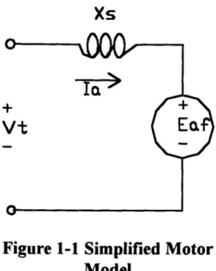
system it will continue to generate an internal voltage, Eaf, until the field comes to a stop.

In wound field machines the field circuit breaker can be tripped simultaneously with the

main circuit breakers thus essentially eliminating the field. Figure 1 shows a simple

Xs

lIi

Figure 1-1 Simplified Motor

Model

The internal voltage generated in the machine is proportional to the rotational

speed of the field. In big machines, such as those used for propulsion or power

generation, these internal voltages can be very large. The generated internal voltage can

be large enough to continue the arcing process and cause further damage while the

machine is coasting down.

The purpose of this research is to develop some tools that can be used to

investigate what happens to a large permanent magnet motor following an internal fault

while the motor coasts down.

1.1 Ship Propulsion Systems

Current naval propulsion systems consist of multiple diesel engines or gas turbines

coupled to one or more propulsion shafts through a set of reduction gears and clutches.

Using two engines per shaft provides redundancy and continuity of propulsion. In the

case of damage or maintenance to one engine while the ship is underway, propulsion can

still be maintained on that shaft.

Although mechanical systems are very simple and reliable, they have some major

disadvantages. Mechanical drive systems require separate prime movers for electrical

power generation. Alignment between the shaft and the prime mover requires that prime

movers be located as low in the ship as possible. This requirement results in large

amounts of"lost volume" inside the ship and the superstructure for intake and exhaust

trunks. Some of this volume can be recovered in ships with electric drive.

Relatively light prime movers, such as gas turbines, can be located higher in the

ship as electric drive does not require alignment between the propulsion motor and the

prime mover. Conceivably, prime movers could be located in the superstructure.

Locating the prime movers higher in the ship can minimize the arrangeable volume lost to

long exhaust and intake trunks. Other advantages and drawbacks of these systems are

discussed in [4].

Another possibility that electric propulsion offers is the capability to move the

propulsion motors outside the hull of the ship.

1.2 Permanent Magnet Motors

The machine used in this research is a permanent magnet ac synchronous motor.

This is essentially an ac synchronous motor in which the field windings have been replaced

by permanent magnets. The analysis used for this machine is that used for wound field ac

synchronous machines assuming that the machine is excited by a field current of constant

value.

Permanent magnet machines have a number of advantages over wound field

and the power losses generated in these windings. In addition, since no electrical

connections are required to supply the field, this eliminates the need for slip rings and

brushes. Therefore, eliminating the field windings can also result in smaller machines than

wound field machines. This is especially important in marine applications that are volume

limited where space is critical.

Some of the limitations of permanent magnet machines come from the permanent

magnets themselves. Excessive currents in the motor windings or excessive heat could

result in demagnetization of the magnets. Other limitations and advantages of permanent

magnet machines are discussed in detail in [5] and [6].

The control aspects and the electrical power requirements of permanent magnet ac

machines are not addressed in this research. Such aspects of permanent magnet and other

electrical machines are addressed in references such as [7] and [8].

For the purposes of this research the permanent magnet motor will be assumed to

have been operating in steady state at the time the fault is initiated. After the fault is

initiated the motor will be disconnected from the rest of the network and allowed to coast

down. This research will only address large, low speed motors such as those that would

be used for ship propulsion. In this configuration the propulsion shaft will be directly

connected to the rotor of the machine.

The permanent magnet motor used in this research is a notional machine. A

notional machine was used as this type of propulsion machinery is not yet in use in naval

One of the advantages of electric drive propulsion is the ability to directly drive a

propulsion shaft without the need for reduction gears. It is desirable that ship propulsion

motors operate at low speeds, so these machines will have a large number of poles. As

the number of poles increases the physical size of the machine will increase. During the

notional design phase an effort was made to keep the size and weight of the motor

comparable with current propulsion machinery. For this research a flux concentrating

permanent magnet machine was selected. The geometry of this machine is shown and

discussed in more detail in chapter two.

1.3 Ship Model

Following the fault to the motor, after the main supply breakers to the motor are

open, the ship is assumed to coast down to some fraction of its initial speed. During this

coast down period and during the initial phases of the casualty it will be assumed that no

action is taken by the ship's crew to slow down or stop the shaft. The basis for this

assumption is that during the initial phase of the casualty, the first indication available to

the operators will be the tripping of the main supply breakers. Once the main supply

breakers trip, there will exist an inherent time delay before action is taken to stop the

affected shaft and take corrective actions. This delay is due to the time that it will take for

ship's personnel to evaluate, recognize and act to combat the casualty.

Automatic protection systems, that operate when the breakers trip, could be used

to minimize the time delay in stopping the shaft. A problem with these systems is that they

could initiate protective action during spurious breaker trips. During these trips protection

The mechanical energy supplied to the motor while the ship is coasting down is

proportional to the speed of the shaft squared. It can be shown that for a given propeller

the rotational speed of a windmilling shaft is proportional to the speed of the ship. As the

ship coasts down the mechanical energy supplied to the motor will decrease as the ship

slows down.

1.4 Faults in Permanent Magnet Ship Propulsion Motors

The focus of this research is investigating the performance of large permanent

magnet motors such as those that would be used for ship propulsion. It can be expected

that part of the electrical protection of these large motors will be main supply breakers.

These breakers will disconnect the motor from its electrical power supply upon detection

of a fault in the motor.

Internal faults are of special interest due to the large amounts of energy that can be

supplied to these motors by a free spinning shaft after the electrical supply breakers are

tripped. Since the field of the machine is supplied by the permanent magnets, the motor

with the free spinning shaft will behave like a generator supplying power to the fault.

Referring to figure 1-1, the excitation voltage, Eaf, is proportional to the flux produced by

the field,

4f,

and the frequency of the field excitation, o [5]

Ef = Kcof

(1-1)

In permanent magnet machines a constant field flux,

4f,

is supplied by the permanent magnets. Therefore to stop this generator action, the shaft must be stopped.

pitch of the propeller in ships with controllable pitch propellers or stopping or slowing

down the ship. Ships with more than one propulsion shaft can use the unaffected shaft to

slow down or stop the ship.

Other ways to slow down or stop permanent magnet machines are discussed in [9].

These methods are for unfaulted machines whose shafts are not being driven by an

external source such as a ship's windmilling propeller. The windmilling propeller and shaft

will rotate at a speed that is proportional to the ship's speed.

1.5 Research Approach

This research studied the dynamic behavior of permanent magnet ac synchronous

motors following an internal fault. The motor studied was assumed to be directly

connected to a ship's propulsion shaft. Following the fault, the motor was disconnected

from its electrical supply source and allowed to windmill as the ship coasted down to a

fraction of its initial speed.

Different from wound field machines, permanent magnet machines have a constant

field flux supplied by the magnets. As the shaft windmills this constant field flux will

generate an internal voltage in the machine. A sufficiently large internal voltage can

continue to support an internal fault in the machine as the shaft windmills.

To accomplish the goals of this research the following tasks were identified and

performed:

1. A notional permanent magnet motor having the performance requirements of a

developed. By specifying the principal motor requirements the motor parameters were

estimated.

2. A dynamic model of the permanent magnet motor, which incorporated the

parameters of the notional design was derived.

3. Models for the internal fault and of the ship were derived.

4. The models of the motor, fault and ship were incorporated into a dynamic

simulation program.

Chapter 2. Conceptual Design

This chapter describes the procedure used to design the notional permanent

magnet motor used in this research. The motor designed incorporates desired attributes of

a motor for naval propulsion. The procedure described in this chapter is implemented into

an Excel [10] spreadsheet, Appendix A. For the motor design, a set of requirements was

established and some initial assumptions were made as to the geometry and operating

parameters of this motor. The initial assumptions and performance requirements are

summarized in Table 1.

Table 1. Motor Specifications

Number of Phases

3

Frequency (Hz) 60 Rotor speed (rpm) 200

Rated power (Hp)

40000

Operating voltage (V) 1000

Power factor

0.8

Winding factor, kw 0.9 L/D 0.22

Tooth fraction, p

0.5

A line frequency of 60 Hz was selected for the motor design since this is the

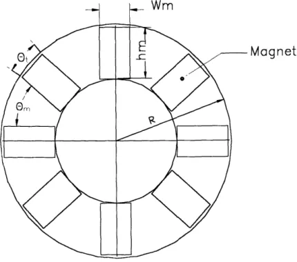
The type of machine that was used in this research is a flux concentrating

permanent magnet machine. In this type of machine the magnets are oriented so that their

magnetization is azimuthal as shown in figure 2-1.

tat

Magnet

Figure 2-1. Motor cross section

Using the geometry described in figure 2-1 and the requirements specified in table

1, some of the initial sizing considerations were started. For the required rotor speed, n,

and electrical frequency, f, the number of pole pairs, p, in the machine was determined

using p = 60f/n. A rotor speed of 200 rpm was selected for this design because this speed

is consistent with rated shaft speeds for naval ships.

Since this machine will be used for ship propulsion, one of its desired attributes is

that it is comparable is size and weight to conventional propulsion machinery. By

feasibility of the motor can be obtained. Weight calculations are performed once all the

machine components are sized.

Once the rated speed of the rotor was established, the radius of the rotor, R, was

determined from the mechanical power output required and the average gap shear

stress, (z). To calculate the radius of the rotor the following two equations were used

Power = (Torque)o

m

(2-1)

Torque = ()(2xRL)R

(2-2)

The aspect ratio indicated in table 1 was calculated using the following relation

suggested by Levi in [10]

2

L

2-L

xUp 3 (2-3)

D

2

The aspect ratio estimated using equation (2-3) minimizes the winding resistance for a

given electromotive force.

Using the aspect ratio, L/D, calculated from (2-3) and combining equations (2-1)

and (2-2), the radius of the rotor is

Power

R =

(2-4)

47o m (':)(L/D) (2-4)

Once the machine radius was calculated, the active length of the machine was determined

as L = 2R(L/D).

A value for the average gap shear was estimated in order to calculate the size of

1

the machine. The average gap shear stress can be estimated by (T) -s BIK , where B1

(rms) value of the effective armature reaction current density [6]. Gap shear has units of

pressure, pascals, (Pa).

For this machine design the value selected for the average gap shear was based on

machine sizing considerations and cooling requirements. By maximizing the gap shear, the

machine radius can be reduced, equation (2-4); however, high values of shear will require

additional cooling requirements.

The value of shear stress selected is that of an air-cooled machine. This type of

machine was selected in an effort to maintain simplicity. For this type of machine, and for

the specified rating, a shear value of approximately 50,000 Pa was obtained [6].

Figure 2-2 shows the variation of rotor radius as a function of gap shear. From

equation (2-4) it can be noted that R oc A-. Higher shear values will result in smaller

machines. However, these smaller machines will require additional cooling provisions,

adding to the complexity and most likely to the overall size of the machine.

Figure 2-2. Radius reduction as a function of gap shear

Fractional reduction in Rotor Size as

a Function of average gap shear

1 .

X

0.8

_

_

-of --- 4 --- --- ---g ---go 0.4 O O m 0 m C 0r 0 I 0 ' 0 'm A e g g a t ( iD 00

Considering the above reasons an average gap shear of 50,000 Pa was selected and

used for the motor design. This shear value is at the high end for typical slow speed

air-cooled machines [6]. For the specified shear and aspect ratio the rotor diameter was

calculated to be approximately 4.2 m and the length of the machine, L, approximately one

meter.

2.1 Air gap size

Mechanical considerations and performance requirements drive the length of the

air gap, g. The minimum physical length, in meters, of the air gap can be estimated from

the following relation [11]

g

3.35 x 1 - 3

( D (2-5)

Using the calculated radius of the rotor, equation (2-4), and L/D, (2-3) a minimum

gap length of 5 mm is obtained. This gap length was used for this research.

2.2 Magnet dimensions

Considering the geometry shown in figure 2-1, and assuming that the magnets

occupy one half of the circumference of the rotor, the width of a magnet is given by

Wm= =-Rand from figure 2-1 wm = 2R sin 0 . Combining these two equations and

p 2

solving for the magnet angle, 0t

0t = 2 sin-

'

2

(2-6)

2p

Om = t (2-7)

P

The remaining dimension of the magnets yet to be determined is the height, hm.

This dimension is determined by considerations other than just geometry, such as the

magnetic flux density at the air gap. In order to calculate the magnet height, the gap flux

density needs to be determined.

In flux concentrating machines, the flux density in the gap is greater than the flux

density in the magnets. To calculate the fields in this machine a simple reluctance model

presented in [ 12] was used. For the given geometry, the flux path in the rotor involves a

magnet and one half of each of two adjacent pole pieces. For one pole piece the

permeance of the air gap is given by

g gap = .oL ROm (2-8)

g

and the permeance of a magnet is

d

m= oL hm (2-9)

Wm

The magnetic flux density in the magnets, Bin, is calculated using a simplified

magnetic circuit. This circuit consists of the magnet's own permeance in series with one

half of the permeance of each of two pole pieces. So that the flux density of the magnets

is given by

Bm= Bo •gap (2-10)

Pgap + g m

2 h_

Bgap =B

2hm

(2-11)

R _m

Solving equation (2-11) for the magnet height, the following relation is obtained

B R

hm= -- Om (2-12)

Bm 2

For a given radius and magnet angle, the ratio of gap flux to magnet flux will

determine the magnet height. The gap flux density that can be achieved in the machine

will be limited by stator teeth and back iron saturation. This limit will be checked later in

the design. Once a magnet height is selected, the magnet spacing needs to be checked.

For the given geometry the closest point between two magnets occurs at the interior

corners. Using simple geometry the distance between two adjacent corners can be shown

to be [12]

7C

s= 2(R-hm)sin--wm cos-

(2-13)

2p

2p

After checking that the magnet dimensions are compatible with the rotor size and

the gap flux density has been selected, the surface current density, K, necessary for

operation of the machine at rated power can be calculated, K

BI

2.3 Determination of terminal current and machine rating

For a machine with a small gap, it can be assumed that the magnetic flux is not a

function of radial position. The space fundamental of this flux is then of the form

4

p(-B, = - sin p B (2-14)

With this value of flux, the internal voltage can be estimated using

E

af2RLN,k.o

af

B

/

(2-15)

2(2-15)

The terminal current into the machine, It, is given by

It - Nslotswslotshslot J (2-16)

6N

where Nslo swso = 2xRXp and K = Jah5,0tks. Once the internal voltage and the terminal

current are known, the rating of the machine IP + jQ = 3VtIt can be determined if the ratio

of terminal voltage to internal voltage, v = Vt /Eaf , is known. A method to calculate v

will be proposed later in the chapter; however, this method requires that the machine

reactances be known.

2.4 Machine Reactances

The permanent magnets are in the main flux path of the armature. The presence of

the magnets will make the machine salient since the direct and quadrature axes will be

affected differently. Derivation of the direct and quadrature axes' reactances is shown in

several places; however, for consistency the notation used in [12] will be maintained. The

direct and quadrature reactances, Xd and Xq, are given by

3 4 oSN2k2RL

p

_O.

Xd = 2

coy

sinR (2-17)

2 x

p g

2

2 P2g 2

These formulas have a new unknown, the number of turns per phase in the stator,

Ns. The value of Ns will be calculated once v and the rating of the machine are known.

2.5 Internal Voltage

To calculate the ratio of terminal voltage to internal voltage the phasor diagram

shown in figure 2-3 is used. A two-axis representation of the machine is shown in figure

2-3. The mathematical transformation used to derive the two-axis model is discussed in

chapter three.

Figure 2-3. Phasor diagram for Negatively Salient

Motor

From figure 2-3 the following set of phasor relations are derived

E

=

Vt2 +(ItXq) -2VtIX sin

Id

= It

sin(y +6)

=

tan-

IXq

cos

V + IXq COS v

(2-19)

(2-20)

(2-21)

d-axis

jXdld

Iq

q-axis

Vt

Eaf = E -(Xq -Xd)Id

(2-22)

To solve this set of equations an iterative method is suggested in [12]. The end

result of the proposed method is a value for the ratio of terminal to internal voltage, v. To

implement the method, the set of equations (2-19) through (2-22) and the machine

reactances, equations (2-17) and (2-18) are normalized with respect to the internal

voltage, equation (2-13). After normalizing, per unit scaling, and some simplification the

reactances are given by

ii0

R

K

pOM

Xad = PI2B ysin m (2-23)

pg B1 2

x- pg

The set of phasor relations after normalizing and assuming operation at rated

current ( it = 1.0 p.u.) and power factor is given by

e'=

v+

Xq

-

2

aqv sin

xv

(2-25)

XaqV COS X/

6 = tan

-

qvcos

(2-26)

v + XaqV

sin

W

id

= sin(W

+

6)

(2-27)

eaf = e* -(Xaq - Xad)id

(2-28)

Using the normalized reactances and the set of equations (2-25) through (2-28) the

suggested method of [12] seeks a set of values that will solve the above set of equations in

which the fixed point is eaf = 1.0. The iterative method is started by selecting an arbitrary

iterations a new value of vnew = Vold/ af is used and the iterative process is continued

until eaf converges to 1.0. Once convergence is obtained the final value of v is used to

determine the machine rating

3VtIt = i -R 2_{LX KB}

1v (2-29)

If a value of terminal voltage is selected, table 1, then the machine terminal current

can be calculated, equation (2-15).

2.6 Stator sizing

Once the terminal current is known the number of stator turns per phase is

calculated, equation (2-16). The slot width and height, the number of slots and the size of

the back iron need to be calculated to complete the initial sizing of the machine. If a tooth

fraction of Xp = 0.5 is used and assuming that R >>g, then the slot width is calculated as

2mtR

w

=6k

(2-30)

6Nk

5

and the number of slots in the stator is given by

Ns,1o = 6NsksXp (2-31)

The slot height, hs, is determined principally by the insulation required by the

armature windings. Commonly these requirements are such that the copper area in the

slot is between 40% to 60% of the area slot [6]. For this design the slot copper fraction,

kcu, selected was 0.5. With these assumptions the slot height is calculated by

h

t =

K

(2-32)

Limits on the current density, Ja, are established by the maximum temperature rise,

0, in degrees Kelvin, above ambient temperature (40 C), allowed in the copper. The

allowable temperature rise is based on the class of insulation used in the machine. For an

air-cooled machine, the maximum current density based on thermal considerations can be

estimated by

Ja <h

'

(2-33)

K

where YCu is the conductivity of copper and h is the overall heat transfer coefficient.

Equation (2-33) represents the energy balance between the heat generated in the copper

and the heat removed by the cooling medium, air [11]. In equation (2-33) an overall heat

watts

transfer coefficient, h = 30 ₀ w was used. This coefficient was derived for an air-K x meter'

cooled machine and is based on empirical calculations discussed in [11].

Equations (2-1) through (2-32) are used in Appendix A to do the initial machine

sizing. Based on the dimensions calculated by these equations and the established machine

geometry, the weight of the machine was estimated. In addition, once the dimensions and

geometry of the machine have been estimated, other machine parameters such as the

machine efficiency and stator leakage reactance can be estimated.

2.7 Stator leakage reactance

The stator leakage reactance was calculated using the methods of reference [ 11].

Leakage reactance consists of (1) slot, (2) tooth top, (3) end winding, and (4) harmonic

synchronous machines with permanent magnet field the gap length is small and tooth top

leakage reactance can be neglected [11].

For an initial estimate, the leakage reactance was assumed to consist of slot and

harmonic leakage reactances. The slot leakage and harmonic reactances were calculated

using the procedure outlined in [ 11]. The calculated reactance was increased by 10% to

account for the effects of end winding reactance in the total leakage reactance.

The leakage reactance was assumed to be the same for the direct and quadrature

axes. This assumption is commonly made in the literature [11].

2.8 Losses and machine efficiency

The power dissipated in the machine determines its efficiency. This dissipated

power will determine the cooling and ventilation requirements for the machine to ensure

that allowable temperature limits are not exceeded. The losses considered in Appendix A

comprise: no-load losses in the iron, friction and windage losses, copper losses and load

losses.

The rotating magnetic field will result in heat losses in the iron due to eddy

currents and hysteresis. These type of losses occur primarily in the stator teeth, the

surface of the rotor poles and the structural parts of the machine exposed to alternating

magnetic fields. These losses are proportional to the square of the peak value of B.

Hysteresis losses are proportional to the frequency and eddy current losses are

proportional to the square of the frequency. Core losses are estimated in Appendix A

Mechanical losses in the machine are the result of friction in the bearings and

windage between the rotor and the stator. These losses were estimated using the relation

presented in [11 ].

The copper losses were calculated by estimating the resistance of the armature

windings and using the rated terminal current. To calculate the armature resistance, the

mean length of conductor per phase in the armature was estimated as suggested in [11].

For a three phase machine the armature copper losses are 3RaI2, where Ra is the armature

winding resistance and I is the line current.

Load losses are caused by the flux produced by the armature currents. These

losses include eddy current losses in the support structures, pole surfaces and damper

windings. The load losses were estimated as 1% of the armature copper losses [10].

The machine efficiency was estimated in Appendix A using

losses

Efficiency = 1-

losses

input

where the losses are the sum of the individual losses described in the preceding

paragraphs. The calculated machine efficiency was 98%, close to the efficiency predicted

by [6].

2.9 Back iron sizing

The thickness of the back iron, hc, must be sufficient to carry the machine flux.

Assuming a sinusoidal air gap flux density, Bgap, the back iron thickness is determined

B. dS =O

(2-34)

If the air gap flux is assumed to be constant, using the specified machine geometry

and if R>>g, equation (2-34) can be simplified to

hc=(Bgap

R

(2-35)

where Bs represents the flux density in the back iron.

The minimum back iron thickness is then calculated by using a back iron flux

density close to saturation. A value of Bs = 1.2 T, rms, was used for the machine design.

2.10 Weight Calculations

A machine weight was estimated by calculating a rotor weight and a stator weight

for the given machine geometry. The material composition of the different components

was assumed to be that of use in standard motor construction. The machine weight

calculated does not include weight of foundations, the weight of a cooling system or the

weight of an enclosure for the motor.

The weight of the motor is expressed in long tons' (Iton) for easier comparison

Chapter 3. Dynamic Models

To perform the fault simulations a model of the permanent magnet motor and of the

electrical fault were derived. These two models were incorporated into a dynamic simulation

model developed by Professor James L. Kirtley, MIT. This chapter describes the various

models used in the simulation. Models for a permanent magnet ac synchronous motor, arc

fault and interconnections between the motor and the power system are presented.

3.1 Two axis transformation

The permanent magnet motor model used in this research is based on the derivations

presented in [11] through [14]. It assumes linear magnetics and sinusoidal stator winding

distributions. Inductance and resistance values for the motor were calculated using the

methods discussed in chapter two and Appendix A.

Using the symmetry of cylindrical rotation, a coordinate transformation that accounts

for the relative motion between the stator and the rotor is introduced. This transformation

maps the stator winding variables to a reference frame that rotates with the rotor. In this

reference frame, mutual inductances are independent of rotor position. Such transformation is

commonly known as the Park's transformation. A version of this transformation used in [5] is

cosO

-sinO

1

cos

2

-sin(O-- )1 1 cos(0+ -)

-sin(

+

3s

1

,/5

(3-1)

where 0 is some arbitrary angle. For a reference frame rotating with the rotor 0 = ot where co

is the speed of the rotor. This transformation is orthogonal and power invariant,

regardless of the choice of angle. The inverse transformation is given by

cosO

cos9y

-X 3 Cos 0 +-)i 3

-sinO

3/n

-sin(

_ 2X

- sin(

+-3)

If the Park's transformation is applied to an arbitrary vector, F, representing a set of

stator variables, such as currents or voltages, the stator variables are mapped to a fixed rotor

reference frame. In this stationary reference frame the machine reactances are constant,

independent of rotor position.

Fdqo = TFabc

Fab. =T-'Fdqo (3-3)

The d and q subscripts are used to represent the direct and quadrature axes,

respectively. The direct axis is aligned with the polar axis and the quadrature axis is aligned

with the interpolar space. Zero-sequence variables are represented by the subscript 0 in

T

-

=

1 1

--.2

(3-2)

equations (3-3). The zero-sequence components represent components of armature currents

that do not produce a net air gap flux [4].

3.2 Per Unit Scaling

The models used in the simulation have been scaled to a per unit (p.u.) system. Scaling

to a per unit system produces variables whose magnitudes are close to one. The base values

selected for this scaling can be arbitrary. However, for this analysis it is convenient to use the

motor's rated power and voltage as the base values for the per unit scaling. Expressing the

motor variables in a per unit system allows the comparison of this motor against other motors

regardless of their ratings.

For this motor the base quantities are defined by

PB= ₂VBIB

ZB=VB (3-4)

B

XB =VB

To convert the motor parameters to the per unit system, the ordinary variables were

divided by the corresponding base quantities. A new quantity will be introduced into the model

to change torque to the per unit system. This new constant is defined as the inertia constant,

H; it represents the rotor's kinetic energy at rated speed divided by the motor rated power.

The inertia constant, H, has units of seconds and is expressed as

1

H =

2

(3-5)

In equation (3-5), J is the moment of inertia of the shat and am. is the shaft's rotational

speed. In general the moment of inertia of a circular shaft can be calculated as J = r2_pdV,

V

where p is the shaft's material density [3]. It can be shown that for a circular shaft this is

equivalent to J = Wk2

, where W is the mass of the shaft and k is its radius of gyration. For a

solid circular shaft of radius, R, the radius of gyration is given by k = R/V . A value for H

was calculated for this motor using the mass and rotor radius calculated in Appendix A.

Since the rotor is directly connected to the propulsion shaft, the length of the shaft and

the propeller needs to be included in the moment of inertia calculation. The weight of the

propeller and of the propulsion shafts can be estimated from propeller and shaft weights from

U.S. Navy ships or commercial ships.

3.3 Permanent Magnet Motor Model

The permanent magnet machine model is defined by a set of six coupled

electro-mechanical equations. The electrical equations in this set are statements of Kirchoff and

Faraday's laws, which describe the voltage-current relations in the machine. The mechanical

equations are statements of Newton's Second Law of Motion. Coupling between the

mechanical and electrical systems is through the dependence of electrical torque on flux

linkages and through the dependence of flux linkages on torque angle, 5.

The machine parameters used for the simulations are calculated in Appendix A using

the methodology discussed in chapter two. A two-axis (d-q axis) representation of the

In the d-q reference frame, the direct axis of the motor is represented by the following

circuit based on the model presented in references [5] and [12].

Ra cXaL

Ifm

Figure 3-1. Direct axis circuit representation

where the constant current source represents the field generated by the permanent magnets.

Similarly the quadrature axis of the motor can be represented by the following circuit.

Ra

Xal

X

Xkq

Rkq

Figure 3-2. Quadrature axis circuit representation

The following notation has been introduced in the above two models:

Xad and Xaq represent the magnetizing reactances,

Xa represents the armature leakage reactance, which is assumed to be equal

for the d and q axes,

Ra is the armature resistance,

\1

Xkd and Xkq are the damper winding reactances, and

Rkd and Rkq are the damper winding resistances.

Using the models shown in figures 3-2 and 3-3, the three phase ac synchronous machine is represented by the following set of equations

Vd = + RaId d- q dt

V =dX

d

RI

+

dt Vkd = d + RkdIkd (3-6)

dt

dhkq Vkq=

dt

+RkqIkq

T.

-

3(%dI

q

- qId)()°

2 c0

For permanent magnet excitation, the field is represented by the constant current source, In. The flux equations for the machine are

Xd = LdId +LadIkd +LadIfm Xkd =Ladd + Lkd kd + Ladlfm

Xq

= LqIq +LaqIkq Xkq = LaqIq + Lkqlkq

(3-7)

where the inductances, Ld and Lq, are defined by

Ld = Lal + Lad

Lq = La +Laq

The simulation code was written to be used with any ac synchronous machine,

unit system. To use the dynamic simulation code, the above set of equations were scaled in the

per unit system. Dividing by the appropriate base quantities, the sets of equations 5) and

(3-6) are represented in the per unit system by

1

r 'dl

vd

I

tXd Xad Xad (3-8)

W kd Xad Xkd Xad

Wtq

LX

q Xaq

I~k~

Xkq

i~kq

1

iq

--

Ix~

(39)

(3-9)

1 d d x co d= - + rai - Wq o dt

1 dq

.

o

Vq

=

q

_ + ra

+

W[d

coo dt

c

o

0

dkd + rkdkd (3-10) w) o dt

0

= d

+

rkqikq

o,

dt

Te = (Wdiq - Vqid)

The damper windings' voltages, vkd and Vkq, were set to zero since these windings are

normally shorted. Using a Thevenin equivalent circuit of the d-axis model, figure 3-1, the

constant current source can be represented as a voltage source, Eaf = X ad fin in series with the

Ra

Xal

Xad

Figure 3-3. Thevenin equivalent of d-axis model

With the model presented in figure 3-3, equation (3-7) can be rewritten as follows

iNdl

_Xd Xadi d eaf (3-11)

[Vkd Xad Xkd ikd eaf/

By solving the above equations for the currents, the d-q model of the motor can then

be incorporated into a simulation code that connects the motor to an external network.

Solving equations (3-9) through (3-11) for the currents, id and iq, and after some simplifications

the following sixth order state-space representation of the motor was obtained

d

d + 4 v Vd (3-12) dt Tad Tad

dWq

Wq

e" Wd + oVq (3-13) dt Taq Taq de_ e" + (X X) - ₊ e (3-14) - ---

i

(3-15) dt Tq'" T"q' q db -dt = o - (3-16) dt L

Eaf

d0 2co (Tm -Te) (3-17)

In equations (3-12) through (3-17) the following quantities are defined:

X ad

eq = d = Voltage

behind subtransient reactance,

X kd

Xaq

ed =q = Voltage behind subtransient reactance,

x

₄

To = Xkd =- D-axis open circuit subtransient time constant,

)

orka

. o rkd

xd

Tad - d = Direct axis armature time constant, Cora

X"

Taq = q - Quadrature axis time constant,

Oo r

X'Xd ad = D-axis subtransient reactance,

Xkd

x2

xi? =x4 _ aq =

Q-axis subtransient reactance,

Xkq

The stator currents, in the motor reference frame, have been defined by

i = dd _tP (3-18)

Xd

iq

Wq d (3-19)

Equations (3-12) and (3-13) are the stator equations, which have time constants of the

order of l/co = 0.0026 seconds. If the transients of interest are in the order of 0.1 to several

seconds then two stator equations, equations (3-12) and (3-13), will become algebraic

equations provided that the following conditions hold

1 1 d

Tad 'Taq dt

Furthermore if co wo, then equations (3-12) and (3-13) simplify to0

Jd Vd (3-12a)

/q = vq

(3-13a)

With these two algebraic equations the machine model has been reduced to a fourth order

model, equations (3-14) through (3-17).

3.4 Network model

The external network model used in the simulation code is based on the model derived

in [15]. This model uses the machine currents to interface with the network. The definition of

the network is accomplished by defining the nodes and branches of the network. This model is

discussed in chapter four.

3.5 Fault Model

The fault model used for this research is an ac arc fault whose properties and

characteristics are described in detail in [2]. Reference [2] describes the electric arc as a

currents. At atmospheric pressure the temperature of the arc will reach temperatures as high as

6,000K.

According to [2], for large currents the arc voltage, ea, is given by

ea = cIi+ 2 +C3i2 (3-20)

i

where the constants cl through c3 are determined by the electrode materials. The

voltage-ampere characteristic of ac arcs will show hysteresis effects with distinct ignition and extinction

voltages [2].

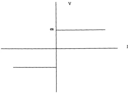
The arc is modeled as a constant voltage drop; for calculation simplifications the values

of ignition and extinction voltages will be neglected. For the materials considered such as

copper and iron the arc voltage drop is approximately 60 volts [2]. The voltage-current

relation of the fault can then be approximated by a characteristic such as that shown in

figure 3-4.

ea

V

I

For the purposes of this research the impedance of the fault is assumed to be much

smaller than the synchronous impedance of the motor. This is simulated by using fault

impedance values ten times lower than the synchronous impedance values for the motor.

The power dissipated by the fault is estimated by multiplying the fault current by the

fault voltage.

3.6 Motor Load Model

The mechanical load placed on the motor by the ship is represented by a mechanical

torque on the shaft. The power delivered by a propulsion shaft for a ship moving at high speed

is proportional to the speed of the ship cubed, P oc v3 [16]. This assumption is not valid for

ships such as destroyers that can reach speeds near or above hull speed2. At speeds close to

the hull speed, the power required may vary with speed raised to a power approaching 6 or 7

[16].

Once a propeller has been selected and matched to the hull, it can be shown the

rotational speed of the shaft is proportional to the speed of the ship. Using this relation, and

since P = To) m then the torque on the shaft can be assumed to be proportional to the square

of the shaft speed. This torque is assumed to be of the form

T, =act } (3-21)

2 Hull speed or critical speed length ratio is the speed at which wave making resistance starts

The constant is calculated with the motor operating at full load using the rated shaft

speed and torque calculated in Appendix A. It is further assumed that this constant is

independent of shaft speed.

A windmilling shaft is not delivering any thrust or torque; however, it will rotate at a

speed determined by the characteristics of the propeller and the speed of the ship. Once the

propeller is selected, for a fixed pitch propeller, the speed of rotation of the shaft, while

windmilling, will be proportional to the speed of the ship. So as the ship slows down the

windmilling shaft will slow down proportionately. To incorporate this model into the dynamic

simulation model it is necessary to determine how the ship's speed changes as a function of

time while the ship is coasting down.

For a ship moving on a constant course at some initial speed, v_, the total kinetic

energy of the ship, U, is of the form U = I Mv2. The symbol M accounts for the mass of the 2

ship and the "added" mass in the direction of motion. While a ship coasts down from some

given speed the rate at which the ship loses energy to the water is equal to the effective

horsepower, EHP, of the ship

dU

= -EHP

(3-22)

dt

In general EHP is proportional to speed elevated to some power, EHP = kv0_{, where k is}

some constant. During a short time interval, At = to - t , equation (3-22) can be written after

some manipulations as

1M(v - v

2

_{) = -(to - t)(kv")}

_(3-23)

If the ship is assumed to be moving at an initial speed, vo, at time, to = 0, then from (3-23)

2 2 2kvn

vo-v = kV t

_=M

(3-24)

For speeds close to the initial ship speed, v v , equation (3-24) can be rewritten as

2kv

2v

t

(3-25)

M

Using equation (3-25) the following relation between ship's speed and time is obtained

1

v

oc

-

(3-26)

Since the rotational speed of a windmilling shaft is proportional to the speed of the

ship, using equation (3-26) the rotational speed of the shaft, Com, will exhibit the same time

dependence as the ship's speed.

If the ship is operating below hull speed, which is the case for most full form ships, then

1

at its rated speed it can be assumed that EHP oc v3. For n=3, then v oc . After the

casualty takes place and the motor main supply breakers are opened, the shaft will continue to

rotate at a speed proportional to the speed of the ship. It can be assumed that the increase in

ship's resistance added by the windmilling shaft is negligible compared to the hull resistance

[17].

Considering the discussion above, while the ship is coasting down, the rotational speed

1

of the shaft was assumed to be of the form co m oC t . The final shaft speed will be

Chapter 4. Simulation Model

With the system model complete, as discussed in chapter three, the dynamic

response of the permanent magnet motor and the internal fault was investigated. The

purpose of conducting these studies was to determine the effect of the internal fault after

the motor is disconnected from the system. The possible damage done by the fault will

occur in a very short time so that the time delay of the relay and protection system might

not be significant.

A possible way to reduce the effects of the fault is to short circuit the motor

terminals after the motor is disconnected from its power supply. By shorting the motor

terminals it might be possible to reduce the power input into the fault, thus serving to

minimize the effects of the fault.

4.1 Discussion of the simulation program

The simulation code was written in C++. Using this language allowed the use of

object-oriented programming (OOP). This type of programming consists of building

programs as a collection of abstract data type instances. Operations performed on the

object types are the abstract operations that solve the problem. These objects serve as

modules that can be reused for solving another problem in the same domain [17]. In the

simulation code generators, motors, nodes and lines are built into objects. These objects

The dynamic simulation program, Appendices B through E, requires the user to

provide four input files. The first two files are used to define the node types and the

interconnection lines between nodes and their reactances. In addition, they define the

nodes to which the generators or motors are connected and the names of the output files

that will contain the node voltages and line currents.

Two other input files are needed for the simulation. One file defines the electrical

parameters of the machine. The other file defines the timing and sequence of events for

the simulation. The machine's electrical parameters used in the simulation were those

calculated using Appendix A.

The simulation code consists of four executable programs that can be run

individually or using a shell program that executes all four programs in their appropriate

sequence. The first program executed is a pre-processor program. It formats the node

and line input data into a format that can be used by the rest of the code. The next

program in the simulation estimates the power flow in the network. It assigns initial

values to node voltages and line currents. Using the power flow equations, the voltages

and current flows of the connected system are calculated.

The third executable program uses the node voltage, line current and power flow

data to build the line data required by the simulation program. The simulation program

will generate three output files that contain the state variables, the node voltages and the

line currents. To perform the simulation the four programs need to be run in sequence

The dynamic simulation program, developed by Professor James L. Kirtley, MIT,

was originally written to simulate the dynamic response of wound field ac synchronous

generators. The generators are defined as objects in the code so that multiple generators,

all possibly different can be connected to the network. For this research it was necessary

to generate a similar object for the permanent magnet motor. To properly interface the

motor object with the other programs it was necessary to maintain the same notation as

that used for the generator objects.

The simulation programs were modified to incorporate the permanent magnet

motor. To incorporate the motor into the simulation program the following major

modifications were made to the simulation code:

1. The state equations for the machine were modified to incorporate the

permanent magnet motor model discussed in chapter three. The reference frame of the

model was changed to the motor reference frame.

2. The programs were modified to delete the voltage regulator associated with

each generator.

3. The ship model discussed in chapter three was incorporated into the program.

This model is used to drive the windmilling shaft after the motor is disconnected from its

power supply.

4. The program was modified to allow connecting a motor to the network.

5. The fault model was incorporated into the motor simulation code. The fault is

introduced at a predetermined time after the simulation starts.

4.2 Fault simulation

The permanent magnet motor model and the parameters derived in chapters two

and three were incorporated into the dynamic simulation model, Appendix E. The

simplified system shown in figure 4-1 was used for the simulations. For this simulation it

was assumed that a single permanent magnet motor was connected to an infinite bus. The

idea of an infinite bus is not applicable to ships' power plants because loads such as

propulsion motors can have ratings comparable to that of the generators.

The infinite bus assumption was made to establish the initial state of the system.

For the simulation, the motor is operating at rated power and rated speed. At the time of

the fault the affected motor was disconnected from the rest of the system so that there was

no interaction between the motor and the rest of the system. Since interaction effects will

not be addressed, the concept of an infinite bus was considered suitable for establishing

the initial state of the system. This bus represented the ship's generators whose output can

be adjusted to provide a specific voltage and power flow.

Using the model shown in figure 4-1, the motor was disconnected from the system

some time after the initiation of the fault. In a real system this would have been

accomplished with circuit breakers together with some sort of sensing system. For this

simulation a fixed time of 100 milliseconds, after the initiation of the fault, was chosen for

the breakers to trip and disconnect the motor from its power supply. This time was used

for all simulation studies.

Once the motor was disconnected from its power supply, it was allowed to

windmill as the shaft coasted down. The speed of the windmilling shaft was taken to be a

function of the speed of the ship, as previously discussed in chapter three.

The fault current and power dissipated at the fault were calculated. The

simulations were terminated after one second. This time was selected for the simulations

since as will be shown most of the power dissipated at the fault will occur within this time.

This is consistent with the results obtained in reference [19]. In addition, this short time is

consistent with the assumptions made in chapter three for the ship model.

Re

Xe

Xa

Ra

Infinite Bus

Figure 4-1. System model

The internal fault in the motor was simulated by assuming that the fault occurred

somewhere in the windings between two points which have generated internal voltages

and leakage inductances. A similar model was used to simulate internal faults in [19].

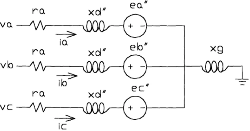
The motor and power supply interconnection model is shown in figure 4-2. This

va

vb

VC

ic

Figure 4-2. Motor and Network Interconnection Model

A derivation for this model and its representative equations are discussed in [15].

For this model it is assumed that subtransient saliency can be neglected, x = xq'. The

internal voltages, ea", eb ", ec", represent voltages induced by rotor fluxes and xg

represents the impedance in the neutral of the machine and of mutual coupling between the

phases. The internal voltages are calculated as follows

o . 1 de" 1 ded

e = -- (e'sinO-e cosO)+ cosO +-sinO d

o co O dt co dt

f? ) 27c 21r 1 27r der' 27 de

eb

=--(e" sin(- )--e"

cos(O- ))+-cos(O- -) + -s

--

)

) ds(O

co,

3 3

o,

3 dt

c-

3

dt

co 27t 27c 1 27c de' _d

e= - - (e sin( + ) - ecos( + )) + cos( + ) +- sin(0 + ) dd

C

co

-3 -

3

dt

oo

3

dt

where, 0 is the shaft angle and e"d and e"q are the subtransient voltages defined in chapter

three. A detailed derivation of this model is explained in [12] and [15].

This machine model was used in the synchronous machine simulation program.

The internal fault was assumed to occur between two phase points whose voltages are

proportional to the internal phase voltage. Because the fault occurred between two

ea"

phases, the voltage across the fault is proportional to the difference between the internal

voltages of the two points.

The internal voltages in the machine are generated across the entire winding.

Since the fault can occur anywhere in the windings there are many possible connections

that can be established. For this analysis the fault was assumed to occur in the middle of

the winding. The impedance seen by the fault will be proportional to the impedance of the

motor winding.

The power dissipated in the fault was calculated assuming that the voltage drop

across the fault was constant as discussed in chapter three.

This type of fault and simulations for a large turbogenerator are discussed in [19].

Fault currents as large as 14 per unit and peak phase currents of approximately 7 per unit

were obtained in [19] for an internal phase to phase fault. These large currents can be

expected to cause severe stator damage.

For an asymmetrical fault, large negative phase sequence currents are expected to

flow in the stator windings and consequently in the rotor damper bars. These large

currents in the damper bars could impose high thermal stresses in the damper bars.

4.3 Simulations

The following cases were run for this research and the results obtained are

presented and discussed in chapter five. All the simulations were started with the motor

operating at rated speed and power. A phase to phase fault was introduced, in all cases,

300 milliseconds after the simulation was initiated. The motor was disconnected from its