A conditional probit model for qualitative choice : discrete decisions recognizing interdependence and heterogenous preferences

Boston

Library

Consortium

IVIember

Libraries

worKing

paper

department

of

economics

A CONDITIONAL PROBIT MODEL FOR QUALITATIVE CHOICE; DISCRETE DECISIONS RECOGNIZING

INTERDEPENDENCE AND HETEROGENOUS PREFERENCES Jerry A. Hausman (MIT)

David A. Wise (Harvard)

Number 173 April 1976

massachusetts

institute

of

technology

50 memorial

drive

Cambridge, mass.

02139

/

A CONDITIONAL PROBIT MODEL FOR QUALITATIVE CHOICE: DISCRETE DECISIONS RECOGNIZING

INTERDEPENDENCE AND HETEROGENOUS PREFERENCES Jerry A. Hausman (MIT)

David A. Wise (Harvard)

Number 173 April 1976

The views expressed here are the responsibility of the authors and

do not reflect those of the Department of Economics or the Massachusetts Institute of Technology.

The authors wish to thank Gary Chamberlain, Zvi Griliches, Charles Manski, and Dan McFadden for helpful suggestions. An earlier version

of this paper was presented at the Third World Congress of the Econometric Society, August, 1975.

M.l.T. Li3RAR''iE3 |

-1-1. Introduction and Background

The social sciences attempt to explain and predict the behavior

of individuals. In practice, this often requires that they predict individual decisions or choices. In many situations, choices are made over a continuum of possibilities; for example, "how much" to spend or

how much to work. But in many other situations, choices are made from

a limited number of possibilities or alternatives; the possible alternatives are "discrete" or "quantal." Indeed, many decisions made in the public sector could be considered to be informed only if knowledge of the deter-minants of discrete choices by individuals were available. Examples

of these kinds of choice are whether or not to work, where to live,

where to work, mode of transportation, and size of family. Knowledge

of the determinants of such decisions is important to the policy maker in designing, for example, income maintenance programs, urban renewal projects, medical education programs, public transportation networks, and child care facilities.

Logit and probit analysis are the most widely used methods for es-timating the relationship between choices on the one hand and attributes of

alternatives and individual decision makers on the other in binary choice,

or two alternative, situations (e.g., Cox [1970]). In multiple alternative situations the most widely used method is a generalization of logit

analysis, often called conditional logit analysis. Professor McFadden has developed qualitative choice models based on the conditional logit specification to a high degree of sophistication. He first applied

the model to the choice of urban freeway routes by state highway departments

[1975] and since has done extensive investigation of transit mode choice by individuals [1974] . Others have applied the same model to college

choice, plant location, occupational choice, and the choice of fuel for

electric power generators. Conditional logit analysis has been preferred over other theoretical possibilities primarily because of computational simplicity, a distinct advantage. The primary disadvantage of the func-tional form providing the basis of conditional logit is a property termed the "independence of irrelevant alternatives." This restriction of the model is quite unrealistic in many situations. To date, attempts to cor-rect for this shortcoming have been on an ad hoc basis and not generally applicable.

This paper proposes a computationally feasible method of estimation not constrained by the "independence" restriction and which allows for a much richer range of human behavior than does the 'conditional logit approach. An important characteristic of the model is the explicit allowance for variation in tastes across individuals for the attributes of alternatives. This gain in realism, though, is at the expense of com-putational simplicity. To date, application of the model is limited to choice situations with four or five alternatives. The example in this paper uses only three. However, the increasing capacity of new generations

of computer facilities may be expected to broaden the applicability of our approach.

The general problem that we are dealing with may be formulated as

follows. Consider an individual who faces J alternatives and must choose one of them. Let the probability that he chooses the j

—

alternative

J

be P., where E P. = 1. Let the outcome be represented by a vector

J

j=l J J

Y = (y-i .y^j• • _{-Yj) J} where y. is either zero or one, and Z y. = 1.

J _j=l -'

Then the probability that the first alternative is chosen is given by the probability that Y = _{(1,0,...,0), where} the probability of any Y

-3-^1 ^2 ^J

is given by P P ...P . For N identical individuals indexed by i, the likelihood that Y^ = _(y^^.y^^'

• • •

'y^j) ' • • • ' "^^ "

^^il'^iZ' ' * "

'^iJ^ '

etc.... is given by the following likelihood function,

N y., y.„ y.

T

eL=

_n

_p/^1

^2 •••Pj •

i=l

If individuals face different numbers of alternatives, J must be indexed by i, and if the i

—

individual is faced with R. repetitions of the

J. 1

same choice situation, then Z y.. = R., and the likelihood function

is given by,

L N R^ y^^ y^2 ^^-^i

^ = _{.", ^il ^12}

_^'y±J.

^

^ _^2 ^

•••^J.

^'

1=1 1 1

A common statistical problem is to find the values of the P. that

maximize the value of this likelihood function. A more general problem

is to allow the selection probabilities to be dependent on attributes

of the alternatives in the choice set and on attributes of the individual making the choice. That is, the probability that the i

—

individual

chooses the _Jj

—

alternative is given by P. . = P(X..,a.), where X.. is

6 ' _ij ^ _ij '

i"^ ' 13

a vector of attributes of the j

—

alternative faced by individual i and

a. is a vector of characteristics of the i

—

individual. Conditional probit analysis differs from conditional loglt analysis in the stochastic specification of the probabilities P . . The probit specification is based

on the multivariate normal distribution, while the logit formulation

rests on the univariate extreme value distribution. In turn, it is useful

to relate the selection probabilities, given the attributes of the alter-natives and characteristics of decision makers, to underlying theories of

consumer choice. While both models can be related to the idea of the

representative individual (explained below) , we will see that the different

stochastic formulations imply quite different theories of individual be-havior and, in fact, lead to quite different predictions of selection

probabilities in some important choice situations. Even though both loodels are likely to "fit the data" well

—

analogous to the similar results

obtained from logit and probit analysis in the binary case; '

the predicted effect of the introduction of a new alternative based on one model is

likely to differ substantially from that of the other. This possibility is

investigated in the last sections of the paper.

Section 2 examines the general specifications of qualitative choice models. The deterministic theory of the representative individual is

discussed and then a stochastic theory is formulated from which the

choice probabilities are derived. In Section 3 specific parametric distributions are developed and conditional probit and conditional logit models are discussed. Section 4 deals with maximum likelihood estimation

of the unknown parameters in the probit model and the formulation of statistics

to compare different model specifications. An empirical example of trans-portation mode choice for commuters is analyzed in Section 5. Important

differences between the conditional probit and conditional logit models are found. In Section 6 artificial data are used to compare forecasts based on the two models when a new transit mode is introduced. One

of the important uses of conditional logit models has been in this situation;

1. We will see below, however, that our model will lead to a covariance

term, for each choice situation, that depends on the attributes of the alternatives being compared

—

the choice set.

-5-thus, the comparative forecasts of the two specifications should be of interest. Again, important differences are found. Finally, the treatment of the "red-bus, blue-bus" problem by logit and probit models is discussed

in Section 7

2. A Model of Individual Choice

While economic theory provides a well-determined axiomatic theory

of individual choice, use of this theory in econometrics is not always straightforward. Even when observations on individual choices are

avail-able, two problems remain. The investigator observes and measures only some portion of the factors that determine individual decisions. There are unobserved attributes of the alternatives in the choice sets faced by

decision makers and unobserved attributes of the decision makers them-selves. Also, the investigator usually lacks repeated observations on choices made by any given individual, in particular, under changing

condi-tions. The usual situation in economics is that data is collected for many individuals, but with only one (random) observation for each. The

follow-ing information is typically available: the observed attributes of the

alternatives in the choice sets faced by individuals, their observed at-tributes, and their choices. In qualitative choice situations with ap-propriate sampling techniques each trial is assumed to be a single drawing from an independent but not identical multinomial distribution. The task

of the empirical investigator is to construct a model of individual be-havior that is consistent with estimation of the probabilities in the

multinomial distribution. The estimation procedure can use only observed

data; but a very important aspect of any such model is the treatment of the

unobserved determinants of individual behavior.

A common procedure used in both economic theory and econometrics

is to assume the existence of a "representative" or "average" individual who is assumed to have tastes equal to the average over all decision maker's with given observed attributes. Suppose the representative individual i

faces alternatives X..(i = 1,...,J), where X,. is a vector of the observed

-7-characteristics of alternative j , and he is described by a vector of

observed attributes a.. Then this representative person is assumed to

1

have a utility function U defined over alternatives X, often assumed linear in parameters, such that,

(2.1) U. . = U(X.

. ,a.)

= _{Z. .3,}

where Z.. is a vector of arithmetic combinations of the elements of

X and a., and g is a vector of parameters. Note, the further assumption

has been made that U(') or, equivalently, 3 is common to the entire

population. This assumption is made necessary by the lack of individual repetitions. If 6 is assumed constant only over subsets of the entire population, the sample would be partitioned according to observed charac-teristics and different utility functions would be estimated for each.

Once a functional fonn representing the behavior of the average individual is given, a stochastic theory is used to describe unobserved components that differentiate a particular individual from the average. That is, the deterministic model, equation (2.1), is assumed to represent average (e.g., mean) behavior, and a nondeterministic part to represent

(random) deviations from this average. A convenient parametrization

of the random utility of alternative j to person i is then (2.2) U.. = U(X..,a.)

+

E(X..,a.) = _Z. .6 + e. .

,

where e is a random variable. Two possible explanations for the stochastic term may be given. The first Is that individuals behave randomly, perhaps due to random firing of neurons; so that faced repeatedly with the same alternative set, the same Individual makes different choices. A more attractive explanation is to assume that given the observed data (X. . ,a )

a stochastic distribution is induced by unobserved data in each trial

of the experiment. That is, there are unobserved characteristics of

the decision maker (or random preferences) and unobserved attributes of the

alternatives. We will discuss this possibility in some detail below.

Given the specification of the utility function U.., the individual is assumed to choose the alternative that maximizes his utility. Suppose individual i faces three choices, J = 3. The probability that he chooses the first alternative is.

(2.3) P., = pr[U., > U.„ and U., > U.„]

il il i2 il i3

i2 il i2 il i3 il i3 il

Similar expressions are obtained for P.„ and ?._. It is clear that i2 i3

the P. . are well defined probabilities once we choose a joint density

function for the e... Let f(e., ,e.„,e.«) = f.(e) be this density function

ij il i2 i3 1

and let F(k.^ ,k „,k.t) be the corresponding distribution function. Then

J:he probability that person i chooses alternative 1 is

/-I /\ n / r 11 i2 Xl r ll l3 ll £, ^ J J J (2.4) _Pii = _{J J /} ^(^il'^i2'^i3^ '^^i3*^"i2'^^il —00 —CO —oo " U.

n+e.,

U.

_„+£.i

f /• 1,12 il r 1,13 il _£, . , _J , = _{/ / /} ' _{f(^il'^i2'^i3>} ^"i3'^'i2'^^il —OO —oo —oo

/ F^(e^^, U.^^2 + _{^il' "i,13} + ^11^ _'^^il

where U. ... is the difference in utility of alternatives j and j' to

the representative individual and F^ = 9F/9k,^. It is sometimes more convenient to look at equations (2.3) and (2.4) in differenced form.

-9-(The subscript i will be dropped and will be used only where needed to prevent confusion.) Then the probability of choosing alternative

1 is,

(2.5) P^ = pr[n23^ < U^2 ^'^'^

"^31 < _^u'^'

where n..i = e. - e... This change of variables will induce a new ioint density g-.(,r]„-.,r\^^) that depends on which probability is being considered

(i.e., g, (•) "f gn(')) . The new density g.(*) is easily derived from the

1. ^ _J

density f(e) by a linear transformation with Jacobian equal to unity, then from (2.5)

,

"l2 "l3

(2.6) _p^ = _{/ / g^(n2i,n33_) cin2idn23}

—00 —CO

Two important points to note are that this transformation reduces the order

of integration by one, and because only subtraction is involved in going from f(') to g.(*)> distributions which are closed under subtraction

or are transformed into mathematically convenient distributions by subtraction may be desirable candidates for f(*)»

The specification of the density function f(e) will complete the

formulation of the model of individual choice. It then remains to estimate

the unknown parameters of U as well as any unknown parameters of f(e).

While mathematical convenience of estimation must be an important consid-eration in choosing the density function f, because equation (2.6) contains

a J-1 dimension integral, a reasonable stochastic theory, represented by f(e)

,

is essential for a model that implies acceptable behavioral characteristics

of individuals. In the next section two stochastic parametrizations are discussed which lead to convenient expressions for the basic probability equation (2.6)

3. Problt and Logit Models of Stochastic Choice

Beginning.with a general formulation, we will discuss first the

conditional probit model; then the familiar conditional logit specification

and its primary disadvantage. The focus of the latter discussion will be

on the parametric specification of the covariance matrix of the joint density function f(e) . The goal is to develop a parametrization with

reasonable behavioral implications that is also computationally feasible,

and that overcomes the main shortcoming of the logit model. An important property of the proposed random coefficients parametrization is explicit allowance for a distribution of tastes among decision makers in the

population. For purposes of exposition, we will consider only three alter-natives.

Following the discussion above, we assume that the values of the

three alternatives to the i

—

individual can be represented by. (3.1a) U(Xj^,a^) = U(X^,a^) + £iX^,a^) = _U^^ + e^^

(3.1b)

U(X2,ap

=

U(X2,ap

+ e(X2,a^) = U^^ + _^12

(3.1c) U(X3,a^) = U(X3,a^) + e(X3,a^) = U^^ + e^^

We may assume, as is usual, that E(e..) = 0, because any nonzero term

would be absorbed in the mean function U...

a. The conditional probit model rests on the assumption that the

e. in equation (3.1) have a multivariate normal distribution. The normal distribution provides a good approximation to many multivariate

distribu-tions, and has the advantage that n..i = e. - e.i is also distributed

JJ 3 J

normally. Suppose then that f.(e) is multivariate normal with covariance matrix given by.

-11-(3.2) E. = X a. , 1.1 1,12 1,2 1,13 1,23 1,3

Consider the probability of selecting the first alternative. The covariance matrix for r\

=£„-£•,

and r\^ = e„ - e,, with density function g-.(.T]j,,T)^),

is given by (3.3) a = 2 2 ^1 " ^13 " "12 + °23 ^1 + ^3 " ^°13 '1,11 "1,12 "^1,22

where the index i has been suppressed. Note that g and 9, are subscripted

according to the alternative whose choice probability is being referenced. Then the probability that the first alternative is chosen is given by.

(3.4) —00

u^^V-i

2 2 +02 -2a^2

\,//o[

2 2 +03 -2a^3 ''l^^21'^31' ^1^ ^^^21^^31

where b^ is a standardized bivariate normal distribution with correlation coefficient r^ =

'^i,i2V"i,ii'^i, 22 = ^^1 " °13 " '^12 + ^23^^

2 2 2 2

(a^ +a„ -2a^ _„) (a, +a„ -2a^_). A further transformation of variables allows (3.9) to be written as

(3.5) ?! = / '

—00 13yw^^22^^"'^l ^

lyi-^i

2 dX,

where (|) is a unit normal density function and $ is a standardized normal

cumulative distribution function. The probabilities P„ and P„ are similarly calculated. The stochastic specification is complete given a parametrization

of the covariance terms, a. . ,^i » in (3.2). With no more than one observation

for each individual, the covariance can be estimated only through para-metrization.

Of course, as mentioned in Section 2, a reasonable assumption may be that the a., are independent. In that case _^^ , for example, has a

particularly simple form given by.

(3.6) fi^ =

'2^2

2

1

^1

+°2

°1

2

2,2

^1 °1

+°3

If the variances are assumed to be equal across alternatives, then the Q.

are identical for all j. And, because the variance terms can only be determined up to a scale factor, we can set them equal to one. The matrix Q then has twos on the diagonal and ones on the off-diagonal. This case

is sometimes referred to as the equi-corr elated case. The independence assumption eases the computation burden of evaluating the integrals in

equations (3.4) or (3.5) considerably. However, computational convenience

is only one criteria for choosing Z; thus, other specifications are also

considered. The problem then becomes one of choosing "good" parametrizations. We will argue below that some rather simple functional forms imply quite

plausible behavioral assumptions about individual decision makers.

Consider again an individual facing a set of alternatives, each de-scribed by a vector of measured characteristics X... As described above, we consider the "worth" to him of each alternative to be composed of two

parts; the "average" worth of an alternative with measured characteristics X. . , plus a deviation from this average, an "error" term. The average

-13-and, over the group of all decision makers, from which a particular individual

is selected at random. The deviation is thus assumed to be a function

of two factors: unobserved characteristics of the alternative together with a deviation in the tastes of a given individual from average tastes,

those of the "representative" individual. We will argue that it may not

be reasonable to assume that these deviations or errors are uncorrelated across alternatives in the choice set for a given decision maker. Indeed,

we will argue that the degree of correlation between any two errors might be expected to depend on how "close" the corresponding alternatives are

in measured characteristics. We will first try to motivate this idea

in a heuristic manner. Then we will discuss possible metrics for measuring "closeness." In particular we will propose a general parametrization of the covariance matrix, simple cases of which are easily seen to capture

the idea of closeness.

For purposes of exposition, let us assume first that all relevant characteristics of alternatives are measured; there are no unobserved attributes. Then the deviation of the utility of any individual from representative utility is due only to differences in tastes across the

population of decision makers. Assume that the preferences, U, of the

average or representative individual over characteristics X^ and X.

are represented by the solid lines in figure 1. The preferences of an individual U are represented by the dashed lines. This individual is assumed to have an "unusually weak" taste for characteristic X„, and thus for the alternative indicated by point A on the graph. He is likely also

to have a "weak" taste for any point such as B that is "close" to A. Knowing his preferences for A, however, may tell us much less about his

Because we don't know the "shape" of any individual's preferences

—

that

is, we don't know how any individual's preferences differ from the av-erage

—

our ability to predict the relationship between any two deviations decreases as the "distance" between them in attribute space increases.

Now assume that all decision makers have identical tastes; but that not all characteristics of alternatives are observed. That is,

the "error" results from the values of unmeasured attributes; that for a given alternative are the same for all individuals, but vary from one alternative to the other. This is true even if measured attributes

of two alternatives, for example, are the same; there may be many values

of unobserved ones. We may expect unobserved attributes to be closer together if observed attributes are closer than if they are distant from each other.

A reasonable argument is based on the assumption that the set of all relevant (to the decision maker) attributes of alternatives has a

multivariate distribution, say normal. If we assume in addition that the covariances between observed and unobserved attributes are not all

zero, the expected value of unobserved attributes depends on the values

of observed attributes. In fact, the expected values of unobserved attributes will be closer together, the nearer are observed characteristics. This

can be seen by considering the expected value of unobserved, given observed attributes, when both groups are jointly normal.

But does this imply that deviations from representative utility are closer together the closer are observed characteristics? Recall

that representative utility, U(X.) , is the expected value of U(X.), given

observed attributes. Unobserved attributes are "included" in U. The relationships between deviations from U(X) and U(Y) should not depend

-15-on how close X and Y are. In fact, assuming that the rules of random sampling are followed, the covariance of e(X) and e(Y) is zero.

Unobserved attributes, however, should be expected to affect the correla-tion between deviations when tastes vary across individuals.

We will propose a rather general random utility formulation of

the model that captures the essence of these heuristic ideas. Special

cases of the formulation are then discussed. For convenience of exposition, we assume that there are only two measured attributes, X^ and X„. The

analysis can easily be extended to more.

Let,

(3.7) U(X) = U(X,a) + e(X,a)

= _(3^ + e^)x^ + (e^ + B2^^2 "^ _^

= e^x^ + B2X2 +

_^i\

+ ^2^2 "^ _^'

In this specification, U = _B X + B^X., e(X,a) = _B,X + B2X2 + _Y, and

1. More formally, let X and Y be the observed attributes of two alternatives

c c

and let X and Y be unobserved. Assume the observed and unobserved attributes have a joint multivariate distribution (e.g., normal). Then

U(X) = EU(X) = _EU(X,X |X) = _/ U(X,X )dX ,

X'^

and the covariance between e(X) and e(Y) by,

Cov[e(X),e(Y)] = _E[U(X) - _EU(X,X^|X)] [U(Y) - EU(Y,Y*^|y)]

=

E[u(x)-u(Y)] - _{eu(x,x'^|x)-eu(y,y'^|y)} = 0,

g^ , g , and Y ^^^ assumed to be uncorrelated random terms. The random

variables 3 and _3^ may be thought of as random taste parameters

repre-senting the effects of unobserved attributes of individuals. The term _y may be considered to represent "purely" random components of utility

—

unobserved characteristics of alternatives, or purely random behavior on the part of individuals, for example.

Note that the taste parameters g and g are assumed to be uncorrelated. An obvious reason for this is the saving in computation that it allows.

There is, however, a more fundamental rationalization. In some sense we describe alternatives by their attributes to allow explicit description

of why one alternative may be preferred to another. If the tastes of individuals for one "attribute" are correlated with those for another,

it must be that the two attributes have something "in common." If this

common component is in fact identifiable, then we would like to isolate

it by explicit consideration of it as a separate attribute. This would presumably eliminate correlation between the new attributes

—

now more precisely defined. In this sense, precise definition of attributes,

if successful, would lead to defined attributes for which individual tastes are uncorrelated.

The variance of the error term corresponding to the j

—

alternative

faced by the i

—

individual is given by,

(3.8) Var(e. .) = a. .^ = a„ ^ X,, .^ + CJ„ ^ X„. .

^ _{+ a}

. .^

ij ij _g^ lij _g^ 2ij YiJ

2

where a represents the variance in tastes across individuals relative

^1

to the measured characteristics, X , etc... The covariance between the

-17-i

—

individual is given by,

(3.9) Cov(e..,e..,) = a„ ^ X, ..X, ...

+

a- ^ X„..X„. .,.

ij ij _3j^ lij lij _{&2 ^^J ^^J}

Because the variance of e is identified only up to some arbitrary multiple,

2 2 2

we can fix one of the variances, a . a_ , or a , at an arbitrary

^1 ^2 ^

2 2

value. We have elected to set o . .

=1.

We must estimate only a„

YiJ 3,

2

and a . In general then the covariance matrix Y. is of the form,

^2 V 2 ^ 2 ^ 2 I

\

\il

^

%il

(3.10) Z. = _^ a

2x^.^x^.2

^a

_'X^i2'-^V2'

k k k k

lX^\il\l3

_1%J\±2\±3

I

%J

\i3^

^ _'yt3' k k k k k k

where the summation is over all measured characteristics. ' _{Note that}

the y . are assumed to be independent across alternatives faced by a given

individual, as well as across individuals.

2

If tastes do not vary across individuals

—

that is, if a

=0

'^k

2

for all k

—

and we assume that the a .,

=1

for all j, then.

(3.11) E^ = 1

1

1. This specification thus allows an "alternative set" effect as used by McFadden [ ] . The logit and Independent problt assume this effect to be zero.

and.

1 2

(3.12) Q. =

J

2 1

for all choices j. This is the independence case.

We mentioned above that the variance in the values, or utilities, that different individuals assign to any particular alternative, or alter-natives with the same measured characteristics, can be thought of as

resulting from two factors

—

differences in tastes across individuals, and unobserved characteristics of the alternative. (This ignores the

possibility of purely random behavior.) Some idea of the relative

im-portance of these two factors can be had by comparing the estimates

2 2

of the normalized a„ with the normalized value of a , fixed at 1.

The number of parameters to estimate can be reduced and the model

2 2

simplified by constraining a to equal some constant variance a„

for all characteristics k. For this simplification to be at all reasonable certainly requires that the variables X, be normalized, since the units

in which they are measured is completely arbitrary. We experimented with this constrained model after normalizing measures on the X, by dividing them by their respective sample standard deviations (determined from measures across all alternatives and individual decision makers in

the sample)

We can constrain the covariance specification even further by assuming that there are no unmeasured characteristics that affect individual

de-2

cisions and setting a

=0.

That is, we assume not only that the variance in tastes is the same for all measured attributes of alternatives, but

-19-also that all the randomness in utility results from variation in tastes. This formulation in fact allows a straightforward intuitive feeling for the properties of the more general model. The relationship between

this specification and the loose idea of the correlation of errors de-pending on "closeness" in attribute space is easily seen. In this case, U(X) is given by,

(3.13) U(X) = B^X^ + _62^2 +

^i\

+ ^2^2'

where U(X,a) = g^X^ + "^^X^, and e(X,a) = _B^X^ + &^X^. If _6^ and _6^

have equal variances and are uncorrelated, the covariance between any

two errors, say for the alternatives X and Y, is given by: Cov[e(X) ,e(Y) ] =

2

a (X,Y + X„Y ) . The correlation between the two is given by,

o^(X Y +X Y ) X Y + X Y

(3.14)

_p^

= - ₌

||

J

| iIy II

= cos(X,Y) .

Jo^iX^hx^^) Jo'^{Y^+Y^)

This formulation assumes that if A and B have the same measured char-acteristics, a decision maker will treat them as identical; the deviation

of his valuation of A from that of the representative individual will equal

the deviation in his valuation of B. (See figure 2.) If there were no

unmeasured characteristics of alternatives, we would want precisely this

property. Identical alternatives are treated identically by a given de-cision maker. '

(We will see below that under this formulation, adding

1. It also has the property that if A and B are orthogonal, or at right angles to one another, so that A^B^

+

A„B„ = 0; the corresponding devia-tions are assumed to be uncorrelated. Finally, if two alternatives are in

the same direction, but different "distances" from the origin, like A and

D, they are assumed to have the same correlation as alternatives closer together, like A and C, or two alternatives A.

an alternative identical to an existing one will not change the predicted probability of choosing other alternatives. This represents the absence of

the unwanted "independence of irrelevant alternatives", property; however,

it is an extreme case, stronger than we would like to impose.)

In summation, we will experiment with three parametrizations of the

covariance matrix. The first constrains all off-diagonal elements to

be zero. We call this the independent probit case. The second assumes

that off diagonal elements are given by (3.9). We refer to it as

co-variance probit. And, third, we will use an intermediate parametrization that constrains the taste variation parameters to be equal. The more flexible parametrizations correspond to letting the data "choose" the

degree of association of e.. and e... conditional on how "close" the

observed alternatives are in attribute space.

These three parametrizations of the covariance matrix are all generali-zations of the "probit" model used often in economic analysis. To date only the independent probit model has been used in the binary choice case where

its properties are rather similar to the more commonly used logit model because the distribution functions on which the models are based are sim-ilar except in the extreme tails. However, with three or more alternatives

the behavior of the logit and covariance probit models is apt to differ since the logit model is based on binary comparisons while the covariance probit model is based on an n-way comparison with interdependent stochastic

terms. In particular, predicted effects of the introduction of a new

alternative are likely to differ substantially between the two models. But before comparing results from the two models we will review briefly the

-21-b. The conditional logit specification is based on the assumption

that the e. in (3.1) are independently and identically distributed with extreme value density functions (Type I extreme value

—

Johnson and

Kotz, pp. 272 ff) , -c . -e. _ 1 (3.15) f(e.) = e ^ _e ^

and distribution functions,

-k.

-e ^ (3.16) F(k.) = pr(e. < k.) = e

It is the limiting distribution (as n->^) of the greatest value of n

in-dependent and identically distributed random variables. While it is dif-ficult to argue that the extreme value distribution is a particularly good representation of the stochastic nature of the e., it turns out to be

ex-J

tremely convenient mathematically. The difference between any two random variables with this distribution [e.g., n. . « = £.. - e... in equations (2.5)

and (2.6)] has a logistic distribution function, that gives rise to the binary logit model. For example, if only two alternatives are available, the probability that the first is chosen is given by.

"l (3.17) P^

^—

"l "2 ,

,

^2 -"l e + e 1

+

e

The probability that the first is chosen from three alternatives is given

(3.18) P, =

^—

' "l "2 "3 ,

^

"2 - _{"l "3} - "1

e+e+e

1

+

e

+e

which appears as a straightforward extension of the binary case. This simple form arises because the relevant probabilities in equation (2.4)

are independent, as well as having convenient functional forms.

That is, Fj^(kj^.U^2 "^

'^l' ^13

"^ _^1^ " f(k^)-Pr(e2 ₁ U^2 "^ kj^)-Pi^(e3 ₁ Uj^3 + k^^)

= f(k,)'F(U + k )'F(U „ + k ). The integration in (2.4) is essentially taking a weighted (by f(*)) average over the values of e^ , of the product

of binary comparisons, where the value of e, is fixed in each. Another way to see that the model assumes that only binary comparisons need be made is to rewrite (3.18) as the inverse of the sum of binary odds. That

is P can be written as,

"1 ^2 U3

(3.19) P = 1/

^—

+

^—

+

^—

.

^1 ^1 ^1

e e e

(The extension to a greater number of alternatives is straightforward.)

In fact, we can let any alternative be a "basis" for the set of alternatives, and then write any probability P. in terms of binary comparisons with

it as.

1. McFadden [1973] has shown that a necessary and sufficient condition

for the random utility model with independent and identically distributed errors to yield the conditional logit or "strict utility" model, is

(3.20) P. = J -23-u. - _c^ "l - "l "2 - "l "3 - "1 e + e + e

Thus all choices may be assumed to result from binary comparisons with

a basis alternative. Well defined probabilities are obtained by appropriate

U. - U^

transformation of these "comparisons" (differences), e , and normalization.

We emphasize the binary comparison aspect of this model because it is

integrally related to its primary shortcoming. This very powerful simplifica-tion brings with it very restrictive assumptions on individual behavior.

As Luce and Suppes [1965], Marshak [1960], and McFadden [1973] have

pointed out, the relative odds of alternative j being chosen over

alterna-tive j' is independent of the number, or attributes, of other alternatives in the set. This so called independence of irrelevant alternatives

assumption follows directly from equation (3.18)

.

While for many problems the logit choice model is adequate, for

some problems which contain alternatives that are close substitutes for

each other the specification is too restrictive. For example, consider an individual with a choice of two residence locations, say Florida

and Vermont. Assume that he likes the sun in Florida; but he likes equally the beautiful fall and winter skiing possibilities in Vermont. This results in a 50-50 chance that he will choose Florida over Vermont; P„T . , /P„ _^ = 1. Now assume that his alternative set is expanded

Florida Vermont

to include New Hampshire, which we assume to be identical to Vermont in skiing opportunities and fall beauty; U(Vermont) = _{U(New Hampshire)}

.

We would expect that the individual would still choose Florida with prob-ability .5 and would choose Vermont o£ New Hampshire with probability .5

and each of them with probability .25. Contrary to this expectation, the

conditional logit functional form constrains the odds of choosing Florida over Vermont to remain at 1. The probability of choosing Florida, as

well as the probability of choosing Vermont, falls. The model predicts

that each state will be chosen with probability 1/3. In the empirical application used later there are three alternatives for commuting to work: drive alone, car pool, or bus; the characteristics of the first two alter-natives are similar. Yet, if we had started only with the drive alone-bus split and wanted to predict the effect of car-pooling, the relative odds of the original choices would be constrained to remain the same, while it

seems likely that much more substitution exists between driving alone and car pooling than between taking a bus and car pooling. These restrictions essentially result from the assumption of independent errors in (3.1). The goal of the conditional probit model is to allow relaxation of these re-strictions.

The probit and logit models have been specified in terms of the theory

of a representative individual and a stochastic theory of the distribution

of "deviations" from the representative individual. On prior grounds it is difficult to choose between them because a more general specification is

gained at the expense of computational convenience. After discussing the

estimation procedure for the probit model in the next section, an empirical example is used to demonstrate differences between probit and logit models

in estimation and prediction. We might expect the independent probit and

the logit models to have similar properties and, in fact, they lead to

almost identical empirical results. Both assume Independence and after normalizing the variances, the distributions that form the basis of the

-25-models

—

independent normal and extreme value respectively

—

are quite similar. The independent probit is introduced to allow direct comparison (nested hypothesis testing) with the covariance probit. Although we can only make "precise" comparisons between the two probit models, the fact

that the independent probit and the logit models give almost identical results allows us in practice to make implicit comparisons between the

4. Estimation

Given a random sample of individuals, the unknown parameters are estimated by maximum likelihood. A sample (without repetitions) may be thought of as N independent drawings from a multinomial distribution with log-likelihood function.

(4.1) N L = K + E J ^ y i=i j=i . . log p.

where y. . = 1 if person i chooses alternative i, and y..

=0

otherwise.

Both the probit and logit likelihood functions have this same general

form, but have different specifications of the probabilities p... Estima-tion of the logit model (equation 3.4) is discussed at length by MacFadden

[1973] and will not be described here. In the case of three alternatives,

the relevant probabilities for the probit model are given by equations corresponding to (3.9) or (3.10) with the bivariate distributions having the covariance matrices

(4.2) a^ = ^2 = 2

2^2

2

%1

"

%2

^

_.\%.

_^\±

-^2i> 1=1 1 2

\i^

+

%2^

"^ _^ ""e ^^^''^ ~ ^''^ i i 2i li^

v'-''°e.'^^2i-^ii)(^2i-Si)

2 2 '^ ₂ y1 y3 _{^^^ 3^} li -

hi\

V'-'%3'-^^^6.'(^2i

' ' 1 1 X3.) f^- =

^l'

+

_{^3'-^^\'(Si-^li)'}

%3^

"^ _^

%

^^^^^_3i " ^1-)^^-^-_li'

^31

- ^o.)21' 2 2 2 y2 y3 _^ B^ 31

V

-27-The derivatives of (4.1) with respect to 3 yields,

„T N J y.. 9P..

k 1=1 j=l ij k

The derivatives of the P.. with respect to g have a simple form comprised

of standardized normal densities and distributions. For example, let us

rewrite equation (3.3) as "l2 ^13 (4.4) _^1 ^ i" / h^(r\^^,r\^^; r^) ^1123^^1122^ —00 —00 ~ - / 2 2 / 2 where U^^ = _^12''^°1 '^ _{'^2 ~ ^^^12} " ^^il~^i2^ S>/Ja^ + 2 2 ~

and likewise for U^_. Then the derivative has the formula

9Pi (Z,^6 - r Z 6) (4.5)

—

^=

4)(Z,.B) $ ^"-^^^—

L.k

3Bj^ 12 , 2 12 >/l-r^ Z 6 - r Zj^ 6 _ + *(Z,3B) $ _i Z^3j^ .

yi-r/

where <()(•) and $(•) are standard normal density and distribution functions respectively. Thus, in the three alternative case the gradient involves only univariate normal densities and distributions that are easily evaluated on a computer. To obtain likelihood values requires evaluation of bivariate normal distributions. This is done using a modification of an algorithm first introduced by Owen [1956]. Each additional alternative past three increases the order of the integrals in the derivatives by one. Thus computation with many alternatives may be prohibitively expensive. To

date, the specification has been used for three and four alternatives and costs have been moderate. Significant cost reductions do accrue to careful programming of the maximization routine. In the case of the

un-2

known a. entering the covariance matrix, the corresponding derivative again has a simple form. For example, the derivative of P, with respect

2 to a. is given by, ^^1 ^,~ , , z e - r z e z e ^'^i^u 9a^_2 12 _y _ ^ 2 ^'"11 ^^6.2 Z, „3 ~ r.Z,„3 Z,o3 3(i)-| 99

/^

22 ""3^ ^12^ - ^iZi33 1 3r^ + <i>(Zi33) *

:===

—

•

7==

•

_^t:^

.

y^

- ^1'

_/i-'^i

where the last term may be written as.

2 3,

bT(ZT„3, Z,,3;

rj

^"1,12 _J^l ^'"1,11

_Jl

^'"1.22 1' 12^'

_'^W'

_^r

J 9a- 2 2(x), _,, da. 2 2ui. .. 9a- 2

,22 ^i ' "i ' "i

The method used to maximize the likelihood function is that proposed

by Berndt, Hall, Hall, and Hausman [1974]. It requires only first derivatives, each iteration is guaranteed to increase the value of the likelihood function

and, given an additional requirement likely to be satisfied (equation 2.1 of Berndt et. al.) , will converge to a stationary point. If a global

maximum of the likelihood function L* is assured, then under the usual regularity conditions (see Cox and Hinckley [1974]) the maximum likelihood estimates will be consistent and asymptotically normal. The asymptotic

-29-covariance matrix of the maximum likelihood estimates is equal to the

covariance matrix of the gradient of the likelihood function evaluated at

2

the maximum 6* = _(gjO )*. The expression,

N ^(^ ^ij ^°S ^ij^ ^(^ ^ij '°^

^j^

(4.7) Q(e) = Z

-J-^^

-J-^^

,

1=1

has the same expectation in the limit as the covariance matrix of the

gradient and thus provides a consistent estimate of the inverse covariance matrix of the parameters.

Given the covariance matrix of the estimates, large sample tests of coefficient values can be made in the usual way. The diagonal elements of the inverse of the covariance matrix of the gradient provide consistent estimates of the variances of the unknown parameters. Tests on model specification can also be constructed. One interesting test of the model specification might be that 6 = (3,a) = 0. Then P. in equation (4.4)

equals

—

and the log likelihood function (4.1) takes the value

(4.8) L' = N log

J

= N log

^

.

Hypothesis testing then follows the classical likelihood procedure with

2

-2(L'-L*) "^ _{XoTT.o .} where K is the dimension of g. For the independent

2

covariance specification where o).

11

= 1 and the a.

=0

are assumed zero, 2

the appropriate test statistic is -2(L'-L*) '^ _Xxr •

K.

Unfortunately, in trying to test the probit against the logit specifica-tion a problem arises. Although both model specif icatons are intended

to estimate the same multinomial probabilities in the likelihood function

classlcal likelihood ratio tests cannot be applied. While the two different likelihood values give some indication of how successful the respective models are with respect to the sample, no easy distributional theory can be developed to choose between the specifications. However, since the

logit specification gives such similar results to the identity probit specification which is a vested case of the more general covariance specification, the relative likelihood values might be used in an

"ap-2

proximate" _x test.

To test the two different classes of models a measure of fit against

the observed frequencies can be constructed. Let,

N J (y.. - p..(e))^

(4.9) Z = Z Z

-^

^

.

i=i j=i p^^(e)

N J

2

Then as I Z p.. becomes infinite for each j, Z approaches the x

i=l j=l ^J

distribution with N'J - (K+1) - N (because probabilities add to 1) degrees

of freedom.

An alternative interpretation of the measure is that under random sampling each individual in the sample is given the same weight and the proportion of decision makers selecting the j

—

alternative is estimated to

be,

(4.10)

_Pj=i

j,

Pij(^>-We note that while predicted frequencies from both the logit and probit models can be compared to the observed frequencies, this does not provide a

formal test of one model specification against the other. An associated nondistribution test is to compare the Z statistics from the three models.

-31-Alternatively, the p. can be compared to the observed p. where p.. = 1

if individual i makes choice j and is zero otherwise. Since given correct

model specification the estimated empirical distribution function converges

to the underlying population distribution function, comparing the estimated

p. to the sample p. provides some guide to relative model performance.

In the next section both probit and logit are estimates, based on

transportation mode choice data, are presented. The models are compared on

5. Empirical Example: Transit Mode Choice

Disaggregate models of transit mode choice are widely used to analyze factors that determine the type of transportation individuals use. The models are important in answering two types of questions: patronage of

a new transit mode (e.g. new subways in San Francisco or Washington) and effects on patronage of changes in existing modes (e.g. introduction of off-peak fares in Boston) . To date, almost all such models have been

based on a conditional logit specification. The major weakness of such a

specification is that when a new mode is introduced or the characteristics

of an existing mode change, all predicted probabilities of choice are

constrained to change by the same proportion. This result follows from the

independence of irrelevant alternatives assumption. While on the micro level of the individual, this property seems undesirable, it is not clear

that aggregate forecasts will be seriously wrong. Therefore, both probit and logit specifications are used to estimate mode choice for commuters to

the central business district (CBD) of Washington, and in the next section

a forecasting example is discussed.

Three alternative transit modes are available in this example. * _The

first mode is driving alone, the second is car pooling, and the third

is public transit (bus). The model analyzes the worker's choice of travel mode from his home to his work place in the CBD. As the model of the

representative individual postulates, two types of factors are important:

1. We would like to thank Professors M.E. Ben-Akiva, F. Koppelman,

and S.R. Lerman for kindly providing us with the survey data used in this

-33-characteristics of the alternatives, x... and attributes of decision makers, a.

,

1

The data used in the study are from the Washington Council of Govern-ments Home Inter\fiew Survey described in [4] . The specification is similar

to that used by Koppelman and Watchnatada [1975]. Three mode

character-istics, and one personal attribute are used. The mode factors are cost of

trip divided by income (PINC) , in-vehicle travel time (INTIME) , and

out-of-vehicle travel time (OUTTIME) . Cost and travel time are typically found to

be the most important determinants of transit mode choice.

Three models are initially estimated. The first two are probit models corresponding to independence and a covariance specification where the

2

alternative specific variances are set to one (a . = 1) . Lastly,

condi-tional logit estimates are obtained for comparison purposes. One hundred observations are used with the cost of computing being quite small (under

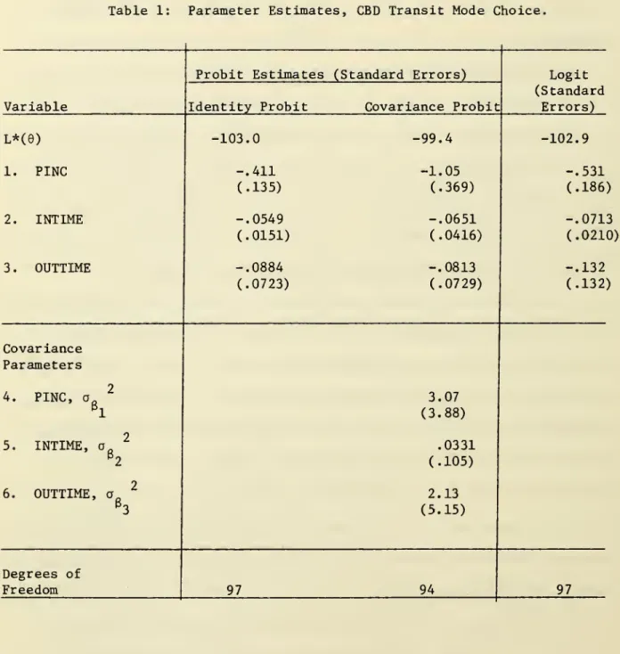
$10 in all cases) . Parameter estimates are presented in table 1. The

parametric estimates of the probit model are roughly similar and accord with prior expectations with respect to sign. Note that the mean estimates are quite different for the probit estimates depending on the specification

of the covariance matrix.

The hypothesis that

6=0,

[L' = -109.89

—

equation (4.7)] is

re-2

jected at the 1% level by all the models using a _x variate with 3 or

6 degrees of freedom. Another important test is a "saturated" model

specification referred to as the presence of "alternative specific effects" by McFadden ([1973], p. 114) or as the "pure mode preference effect"

([1973], p. 131). This test entails inclusion of a constant for the

Table 1: Parameter Estimates, CBD Transit Mode Choice.

Variable

Probit Estimates (Standard Errors) Identity Probit Covariance Probit

Logit (Standard Errors) L*(e) 1. PINC 2. INTIME 3 OUTTIME -103.0 -.411 (.135) -.0549 (.0151) -.0884 (.0723) -99.4 -102.9 -1.05 -.531 (.369) (.186) -.0651 -.0713 (.0416) (.0210) -.0813 -.132 (.0729) (.132) Covariance Parameters 4. PINC, a e. 5. INTIME, a. 6. OUTTIME, a. 3.07 (3.88) .0331 (.105) 2.13 (5.15) Degrees of Freedom 97 94 97

-35-left out of the model specification, e.g., a "convenience factor" for

driving alone versus car pooling or taking transit. Besides providing

a check for correct model specification, this test is important since forecasting the effects of the introduction of a new choice or altering

the characteristics of an existing mode are impossible if alternative specific effects are present. The two saturated models which are tested are first to include alternative specific constants for the second and third choices in the identity probit specification (for choice one the

alternative specific effect is normalized at zero) and second in the

co-variance probit model to have two alternative specific effects and to

2 2 2

estimate a „ and o _ while normalizing a ,

=1.

Neither saturated

y2 y3 yl

model provides a significant improvement over the corresponding unsaturated model at the 10% level by a likelihood ratio test although some evidence

is present that there may be a specific effect for the transit choice.

Thus the model specifications would be appropriate to use in a forecasting situation.

Variable L*(e) 1. PINC 2. INTIME 3 OUTTIME 4. Alt. Effect 2 5. Alt. Effect 3

Identity Probit Covariance Probit

-101.2 -98.9 -.107 -.187 (.230) (.722) -.0379 -.0216 (.0282) (.0567) -.139 -.246 (.073) (.877) -.033 -.047 (.496) (1.11) .483 .361 (.403) (.460) Covariance Parameters 6. PINC,

a^

.098 (.529) 7. INTIME,

a^

.0054 (.024) 8. OUTTIME, aJ" .204 (.782) 9. Alt. Effect 2, a

_^

2.02 (3.46) 10. Alt. Effect 3, a

^

1.001 (8.42) Degrees of Freedom 95 90 Unsaturated LR Statistic

-37-The two unsaturated probit specifications can be tested against each other in two ways. First a likelihood ratio test can be constructed.

2

Two times the likelihood ratio is distributed as _x with three degrees

of freedom. This statistic has the value of 7.2 which is significant

at about the 7% level. The more general specification seems to provide evidence of considerable variation in tastes for the first and third mode attributes. A second test of the covariance specification as well

as the logit specification is to calculate the predicted sample frequencies

as discussed in Section 4.

Estimated Sample Frequency Distribution

Mode 1 Mode 2 Mode 3 _X2

Independent Probit .362 .218 .421 1.67

Covariance Probit .346 .197 .457 .281

Logit .363 .218 .419 1.73

Sample .34 .18 .48

Two findings should be noted. All model specifications do a good job with the hypothesis of the predicted and empirical distributions not

being significantly different not rejected in all cases. Also, as expected,

the independent probit and logit specifications give virtually identical population forecasts. The covariance probit specification, however,

2

does better than either of the other models. Not only is the x statistic

lower, but also it never misses the sample frequency by more than .02. Given the wide variation in transit mode choice, these results appear promising for further development of the model.

6. Forecasting Example: Introduction of a New Transit Mode

Disaggregate mode choice models are often used to forecast patronage

for a potentially new transit mode. Transit modes are described in terms of their characteristics x... If a new mode is introduced its characteristic

ij

vector X. ^,, along with the individual attributes a, will be used to form

1,J+1 ° 1

the representative utility U. ^ = Z. _f,-,&' This utility will then

be compared with the utility of the other modes U. . (j = 1,J and i = 1,N) and

the probabilities of use by each individual will be predicted by the stochastic model.

To ascertain if important differences between probit and logit forecasts might be expected, a new mode was "created" and resulting effects were

predicted with the different specifications. The "new" mode is intended to correspond roughly to a new subway mode. Cost divided by income (PINC)

is set at a mean value higher than the bus mode, the mean of in-vehicle travel time (INTIME) is assumed to be lower than the bus mean, and out-of-vehicle time (OUTTIME) is set at a higher mean. Two types of experiments were carried out. In the first, all x.. for the new mode were set at the

mean values. In the second, not reported on here, a random number generator assigns the x.. randomly according to normal or rectangular distributions.

Of course, in any actual forecast situation the design characteristics of the new mode would be used to set x. ^.,

1,J+1

For the probit models the probabilities of taking the new mode follow from equation (2.6) and are given by.

^41 ^42 "43

(6.1) P4 = _{/ / / ^1(^14'^24}'"^34^ _{'^''l4'^'^24'^34'}

-39-where h, (•) Is a trivariate normal density. For existing modes (say the

first mode) the probability in equation (2.6) changes with the addition

of a new dimension of integration. The new probability, P^ , will be less

than the former probability P, , but no fixed relationship between P.

and the old P. can be ascertained. It depends in a complex way on both

the U... and the covariance matrix of the normal distribution. On the

other hand, the new probability according to the logit specification is

(z^-z^)e

(6.2) I, =

^

4 4 (Z -Z )|

Z e ^

The old probabilities can be seen to change from equation (3.12) only Pi Pi

in the addition of a new term in the denominator so that

^—

=

—

, the

independence of irrelevant alternatives assumption. As discussed above, many people find it unreasonable that for representative individuals the

same proportion will change from driving alone to the subway mode as will switch from the bus mode. However, it is important to realize that this

assumption is a micro one and may not have an adverse effect on macro (population) predictions.

Given the new alternative the macro forecasts that a transit planner might use in designing the new mode are:

Aggregate Probabilities of Transit Choice Mode 1 Mode 2 Mode 3 Mode 4

Independent Probit .335 .200 .391 .074

Covariance Probit .255 .181 .377 .187

The forecasts again demonstrate that the logit and identity probit specifica-tions give very similar results. While the independence of irrelevant

alternative property holds only at the level of individual probabilities, note that the logit specification forecast a ridership of 8% for the new mode with the three existing modes losing ridership of from 7.9% to 8.3%.

Thus the independence property holds approximately at the macro level

in this example. The covariance probit forecasts differ in two ways. First, a much greater ridership of 18.7% is forecast for the new mode.

Also, many of the new riders are from the existing transit mode and from those people who currently drive alone. Current mode two which is car pooling has a decline of less than half that of the other two modes. Thus a differential response of the three existing modes to the new

mode is found. While this experiment cannot be validated since artificial data is used, it does demonstrate that the different specifications may lead to different forecasts. Furthermore, both the logit and independent probit models suffer from the disadvantage that more people are forecast to take existing mode two than currently do so in the presence of three choices. These forecasts seem counterintuitive in the presence of an enlarged choice set.

-41-7. Conditional Probit Specification and Random Utility Models

The stochastic specification of the utility function U.. in equation

(2.2) is sometimes called the random utility model. Block and Marschak

[1960] and Luce and Suppes [1965] discuss the model at length, and recently Manski [1975] has given an interesting theoretical discussion of a special case of this model

—

the independent and identically distributed random utility model. By this terminology is meant that the stochastic terms are I.I.D. and thus independent of x. . and a.. The logit specification,

being a particular case of this specification, is often criticized on

the following grounds. * _{(McFadden has called the problem the "red-bus}

blue-bus problem".) Suppose in a transit choice problem the original choice set consists of driving alone or taking a (red) bus. Next, an additional alternative is added identical in all characteristics to the

red bus, except its color is blue. From equation (3.4) it can be seen that the logit specification will "correctly" forecast equal probability

of use of the two buses; but, unfortunately, the decreased proportion

of car drivers must exactly equal the decreased proportion of red bus riders. Thus, the odds of the first two choices must remain identical,

so if the original probabilities were 2/3 car and 1/3 bus, the new probabilities are 1/2 for car and 1/4 for each type of bus. This counterintuitive

result has led to many attempts at "correction" of the logit specification

to remove the property.

Note that the independent probit specification of equation (3.5)

has a similar undesirable property. The original probability of driving

is

1. G. Debreu, to the best of our knowledge, was the first to point out this property, although his example is less prosaic than ours.

U //2

(7.1) _{^1 = /}

*(^2i^ '^'^Zl

where <!)(•) is the standard normal density. When the blue bus is added,

the probability of driving falls to

U //2 U //2 (7.2) _p^ = _/ ^^ _/ ^-^

b(n2i,Ti33^; 1/2) dn3^2'^nj^3

—OO —00

where U „ = U^» since all characteristics are the same. While the exact

relationship between P and P depends on U^„ and follows no simple

formula, as does the logit formula, the result is still counterintuitive. The independent probit specification would not be appropriate in such situations.

On the other hand, the covariance probit specification offers a

solution to the problem. Originally, the probability of driving is

U-„/(2+Za^

X 9^)^^

(7.3) _^1 = _{/ *(^21^}

'^'^21-—OO

With the addition of an identical alternative the probability is

0^2/(2+1:0.^ ^12^^^ U^2/(2+Za.^

_\2^^

(7. A) _{^1 "} / / ^^^21*^31' ^^ '^^21*^'^31'

—00 —00

The correlation is unity since in equation (3.8) oi^

^^ = o)^ ^» = co^ 07 ^^ ^^^

natural assumption is made that the unobserved characteristics are the

same for the red and blue buses and have covariance equal to their respective variances. Because the limits of integration in equations (7.3) and (7.4)

are identical, P = _P-i . The second integration is equivalent to the first

integration along the line rio, = no-, . Thus, the covariance specification

-43-driving remains the same while P„ = P = _{1/2 P„.} * _{Thus the}

model specification seems satisfactory in the "red-bus blue-bus problem".

1. Actually, the probabilities P„ and P„ are degenerate in one dimension,

References

1. Berndt, E.K. , B.H. Hall, R.E. Hall, and J.A. Hausman, "Estimation and

Inference in Nonlinear Structural Models," Annals of Economic and Social Measurement, March 1974, pp. 653-665.

2. Block, H.D. and J. Marschak, "Random Orderings and Stochastic Theories

of Responses," in I. Olkin, et. al. (eds.), Contributions to Prob-ability and Statistics, Stanford, pp. 97-132, 1960.

3. Bock, R.D. and L.V. Jones, The Measurement and Prediction of Judgement and Choice, Holden-Day, San Francisco, 1968.

4. Cambridge Systematics, Inc., The Effect of Transit Service on Automobile Ownership, U.S. D.O.T. Contract DOT-OS-30056, 1974.

5. Cox, D., The Analysis of Binary Data, Methuen, London, 1970.

6. Cox, D. and D.V. Hinckley, Theoretical Statistics, London, 1974.

7. Johnson, N. and S. Kotz, Continuous Univariate Distributions - 1, Houghton

Mifflin, Boston, 1970.

8. Koppelman, F. and T. Watanatada, "Disaggregate Three-Mode Choice Model for Aggregate Forecast Testing," Unpublished Mimeograph, MIT, 1975.

9. Luce, R.D. and P. Suppes, "Preferences, Utility and Subjective Probability," in Luce et. al. (eds.) , Handbook of Mathematical Psychology, III,

Wiley, New York, pp. 249-441, 1965.

10. Manski,

C,

"The Structure of Random Utility Models," School of Urban and Public Affairs, Carnegie-Mellon University, Working Paper, 1975.

-45-11. Marschak, J., "Binary Choice Constraints on Random Utility Indicators,"

in K. Arrow (ed.)> Stanford Symposium on Mathematical Methods in the Social Sciences, Stanford, 1960.

12. McFadden, D., "Conditional Logit Analysis of Qualitative Choice Behavior,"

in P. Zarembka (ed.) , Frontiers in Econometrics, Academic Press,

New York, 1973.

13. McFadden, D., "The Measurement of Urban Travel Demand," Journal of Public Economics, 26, 1974.

14. McFadden, D. , "The Revealed Preferences of a Government Bureaucracy:

Theory," Bell Journal, Autumn 1975.

15. McFadden, D., "The Revealed Preferences of a Government Bureaucracy: Evidence," Bell Journal, Spring 1976.

16. Owen, D. , "Tables for Computing Bivariate Normal Probabilities," Annals

k::'

^t-BEC ^0

^m.'^w^

jj',..

HB31.M415 no.169

Fisher, Frank l/Quantity constraints, s 726267 .D*BKS.. 000198""

3 ^DflO DOO b4b 353

SERIAL-CIRCULATE

MANUALLY

T-J5 E19 w no.170

Temin, Peter. /Lessons for the present

726484 ,.D*B|<S. Oa0,.?.3.ir

liiiiiH

3

TOaa

ODD

bflT MMS

V

HB31.IV1415 no. 171

Joskow, Paul L/Regulatory activities b

727644, D*BKS [)rir)4804S

3 TDflD

DDO

TTO DSfl HB31.IV1415 no. 172

BhagwatI, Jagd/Optinnal policy interven

727641 D*BKS 00048047

3 TDflO

DOO

TTD 074

HB31.M415 no.173

Hausman, Jerry/A conditional probit mo 727640... D*BKS . .. 0004804S

3

TOaO

000

TTO lOfl HB31.IV1415 no. 174

Carlton, Denni/Vertical integration in 727637 P*BKS 00048C

3 TOflO 000 TTO 124

HB31.IVI415 no. 175

Fisher, Frankl/On donor sovereignty an

727636 D*BKS 00048

1

iiiiiii