by
KARA M. HUFFMAN
B.S. Aeronautical and Astronautical Engineering University of Illinois at Urbana-Champaign, May 2004
SUBMITTED TO THE DEPARTMENT OF
AERONAUTICAL AND ASTRONAUTICAL ENGINEERING
IN
PARTIAL FULLFILLMENT OF THE DEGREE OFMASTER OF SCIENCE IN AERONAUTICS AND ASTRONAUTICS at the
MASSACHUSETTS INSTITUTE OF TECHNOLOGY ay 26,2006 sMT
LL\*\? ,.:% 3'3
,kf
2
O 2006 Massachusetts Institute of Technology All rights reserved
...
...
...
Signature of Author.. ./ .".r.y.
,
,
.-.
n
(kl
- U D
Department of Aer autic and Astronautics May 26,2006
-
...
Certified by..
,.
...
.=-. ..
./.
...
Dr. Raymond J. Sedwick Dep ment of Aeron utics and Astronauticsf
h1
4
Thesis Supervisor...
Accepted by..
...
'
Professor Jaime Peraire Department of Aeronautics and Astronautics Chair, Comrni ttee on Graduate Studentby
KARA M. HUFFMAN
Submitted to the Department of Aeronautics and Astronautics on May 26,2006 in Partial Fulfillment of the
Requirements for the Degree of Master of Science in Aeronautics and Astronautics
at the Massachusetts Institute of Technology
Abstract
Star trackers provide numerous advantages over other attitude sensors because of their ability to provide full, three-axis orientation information with high accuracy and flexibility to operate independently from other navigation tools. However, current star trackers are optimized to maximize accuracy, at the exclusion of all else. Although this produces extremely capable systems, the excessive mass, power consumption, and cost that result are often contradictory to the requirements of smaller space vehicles. Thus, it is of interest to design smaller, lower cost, albeit reduced capability star trackers that can provide adequate attitude and rate determination to small, highly maneuverable, low-cost spacecraft. This thesis discusses the analysis used to select hardware and predict system performance, as well as the algorithms that have been employed to determine attitude information and rotation rates of the spacecraft. Finally, the performance of these algorithms using computer simulated images, nighttime photographs, and images captured directly by star tracker prototypes is presented.
Thesis Supervisor: Dr. Raymond J. Sedwick Title: Principle Research Scientist
To Mom and Dad, for teaching me to reach for the stars,
To Jonathan, for being my biggest fan,
and
To my fiance, and soon-to-be husband, Jon,
Abstract
...
3 Acknowledgments...
5 Table of Contents... 7
List of Figures... 13
List of Tables ... 19 Nomenclature...
21 Acronyms...
23 Chapter 1...
251.1 Attitude Sensors for Satellites and Spacecraft
...
251.2 Types of Attitude Sensors
...
26...
1.2.1 Earth Sensor 26 1.2.2 Sun Sensor...
27...
1.2.3 Magnetometers 28 1.2.4 Global Positioning System Receivers...
29...
1.2.5 Star Trackers 31 1.3 The Next Generation of Star Trackers...
36Chapter 2
... 41
...
2.2 Imager Selection 44...
2.2.1 CID Imagers 4 4...
2.2.2 CCD Imagers 4 5...
2.2.3 CMOS Imagers 46...
2.3 Optics Design 4 9 2.4 Hardware Mounting...
53 Chapter 3...
55 3.1 Stellar Signal...
55
.
.
3.2 Noise Vanations...
583.2.1 Signal Shot Noise
...
593.2.2 Dark Current Noise
...
593.2.3 Background Noise
...
59. .
...
3.2.4 Quantization Noise 60...
3.2.5 Readout Noise 61...
3.2.6 Combining Different Noise Types 62 3.3 Signal-to-Noise Ratio...
63Chapter 4
...
654.1 Image Thresholding
...
65...
4.2.1 Formation of Star Clusters
...
674.2.2 LIST and FAR-MST Centroiding Techniques
...
69Weighted Sum Technique
... 69
...
Measuring Centroid Uncertainty 71 Maximum Likelihood Estimator Technique...
73Performance Comparison Between WS and MLE Centroiders
...
77...
4.2.3 Predictive Centroiding 84...
Chapter 5 87 5.1 NASA Sky2000 Star Catalog... 87
...
5.2 Stellar Matching Techniques 89...
5.3 Single Star Matching 90...
5.4 Pattern Matching 93 5.4.1 The Angle Method and Pivoting... 93
5.4.2 Triangle Matching Algorithms ... 95
Spherical Triangle Pattern Matching ... 95
Planar Triangle Pattern Matching
... 97
...
5.4.3 Rate Matching 98 5.4.4 Selecting Stars to Process ... 98...
5.5.1 Pair Match ... 100
5.5.2 Triangle Match
...
1005.5.3 Rate Match
...
1045.5.4 N-vertex Match
...
105Creating a Reduced Star Catalog
...
105Double Star Reduction
...
107Projection of Stars onto the Celestial Sphere
...
108The k-vector
...
109The n-vertex Match Algorithm
...
111Chapter 6
...
1156.1.1 Wahba's Loss Function
...
115...
6.1.2 The Predictive Attitude Determination Algorithm 116...
6.1.3 The q-method and the QUEST Algorithm 117...
6.1.4 The Singular Value Decomposition Algorithm 122 6.1.5 The Fast Optimal Attitude Matrix Algorithm...
124Chapter 7
...
1277.1 Centroider Performance
...
1297.1.1 Centroider Speed
...
1297.1.3 Attitude Quaternion Uncertainty
...
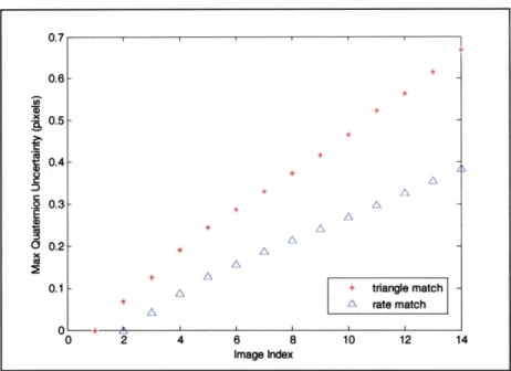
1447.2 Triangle Match Performance
...
1477.3 Rate Match Performance
...
1517.4 Attitude Quaternion Comparison Using n-vertex Match
...
159Chapter 8
...
1658.1 Conclusions
...
1658.1.1 The Optimal Centroider
...
1658.1.2 Pattern Matching
... 167
8.1.3 Attitude Determination ... 170
8.2 Future Work
...
170...
8.2.1 Quantifying Multiple Star Pairs 170 8.2.2 Additional Benchmarking...
1718.2.3 Dynamic Thresholding
...
172...
8.2.4 Predictive Centroiding 172 8.2.5 Reducing Error Propagation in Frame-to-Frame Pattern Matching ... 1738.2.6 Attitude determination
... 173
...
Appendix A 175...
Definition 175...
Quaternion Multiplication 175Frame Rotation vs. Vector Rotation
...
176 References...
. . .
. . .
.
. . .
.
. . .
.
.
.
. . .
.
.
. .
. . .
. . . .
. . .
.
. .
. . .
. . .
.
.
. .
. . .
.
.
. . .
179Figure 1.1 Goodrich Corporation Multi-Mission Earth Sensor Model 13-410[~]
...
27 Figure 1.2 AeroAstro. Incorporation Medium and Coarse Sun ~ensors[~I...
28 Figure 1.3 Voyager Spacecraft with Magnetometer Boom ~xtended'~]...
29...
Figure 1.4 GPS Satellite ~onfi~uration[~O] 30
Figure 1.5 GPS Receiver Block ~ i a ~ r a m ' ~ ]
...
31.
...
Figure 1.6 Star Scanner Example Galileo
acecr craft["'
33 Figure 1.7 Gimbaled Star Tracker Example; Top Left . SR.71. Top Right . RC.135. Bottom .Figure 1.8 Astro- 1 Observatory aboard ~ ~ s - 3 5 ~ ~ ~ ~
...
34 Figure 1.9 Comparison of LIST and FAR-MST Attitude ~eterrnination'~~]...
37 Figure 2.1 ASTROS Tracker Block ~ i a ~ r a m [ ~ O I... 42
...
Figure 2.2 LIST and FAR-MST Star Tracker Block Diagram [291 43
...
Figure 2.3 Fillfactory IBIS5-A-1300 CMOS 49
...
Figure 2.4 Illustration of Defocusing Effects Due to Field Curvature 52...
Figure 2.5 Implementing a Double Gauss Lens to Remove Field ~ u r v a t u r e [ ~ ~ ' 53Figure 2.6 ASTROS Tracker Hardware ~ s s e m b l ~ ~ ~ ~ ]
...
54 Figure 2.7 LIST ~ o u n t ' 471... 54
Figure 3.2 Airy Disk with Outer Rings Digitally Enhanced to Make More Easily visible' 491
....
56...
Figure 3.3 Gaussian Function with Bivariate Normal Distribution 57 Figure 3.4 Standard Normal Distribution Depicting the Percentage that SNR Will Exceed lo. 20. and 30 Amounts of Noise...
6 3...
Figure 4.1 Filtered Image with Threshold Set at SNR = 1 66 Figure 4.2 Bright Star...
68Figure 4.3 Dim Star
...
69Figure 4.4 Centroid Accuracy with No Noise
...
71Figure 4.5 Centroid Accuracy for Various SNR
...
73Figure 4.6 Simulated Noisy Image for Mv = 1
...
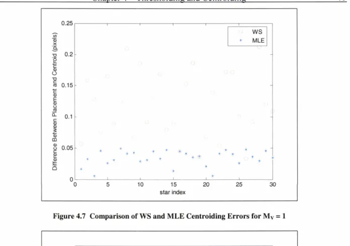
78Figure 4.7 Comparison of WS and MLE Centroiding Errors for Mv = 1
...
79Figure 4.8 Simulated Noisy Image for Mv = 2
...
79Figure 4.9 Comparison of WS and MLE Centroiding Errors for Mv = 2
...
80Figure 4.10 Simulated Noisy Image for Mv = 3
...
80Figure 4.1 1 Comparison of WS and MLE Centroiding Errors for Mv = 3
...
81Figure 4.12 Simulated Noisy Image for Mv = 4
...
81Figure 4.13 Comparison of WS and MLE Centroiding Errors for Mv = 4
...
82Figure 4.14 Simulated Noisy Image for Mv = 5
...
82Figure 4.15 Comparison of WS and MLE Centroiding Errors for Mv = 5
...
83Figure 5.2 Minimum Number of Stars for Given Mv and FOV
...
88Figure 5.3 Difference Between Assigned Mv and Calculated Mv ... 91
Figure 5.4 Stars to Match from Image 1
... 102
Figure 5.5 Candidate Matching Stars from Image 2
...
102Figure 5.6 Candidate Star Matrix
... 103
Figure 5.7 Row Reduction of Candidate Star Matrix
...
104Figure 5.8 All Stars in NASA SKY2000 Master Star Catalog Brighter than MV6 ... 106
...
Figure 5.9 Reduced Version of NASA SKY2000 Master Star Catalog 107 Figure 5.10 Plot of A ... 109Figure 5.1 1 Linear Approximation of Plot of A
... 110
Figure 5.12 N-Vertex Match Example with 4 Stars
...
112Figure 5.13 Results of N-Vertex Match Example
...
113Figure 7.1 Centroiding Execution Times for Noise Threshold of lonoise
...
129Figure 7.2 Centroiding Execution Times for Noise Threshold of 1
.
5anOise... 130
Figure 7.3 Centroiding Execution Times for Noise Threshold of
... 130
Figure 7.4 Centroiding Execution Times for Noise Threshold of 3onOi,
...
131Figure 7.5 Centroiding Execution Times for Noise Threshold of 4onoise
...
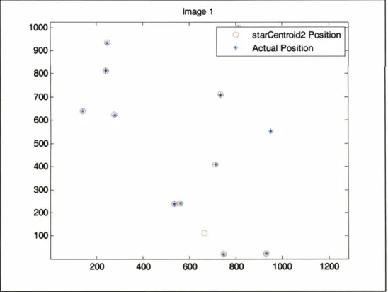
131Figure 7.6 Image 1 . starCentroid2 Positioning Accuracy for Noise Threshold of 1 onoise
...
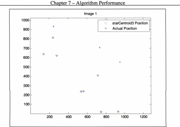
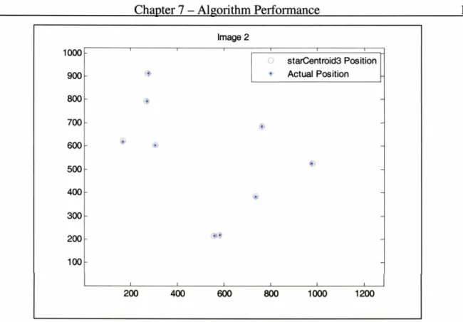
133Figure 7.8 Image 2
.
starCentroid2 Positioning Accuracy for Noise Threshold of lanoise...
134...
. Figure 7.9 Image 2 starCentroid3 Positioning Accuracy for Noise Threshold of 1 anoiSe 135...
Figure 7.10 Image 3 . starCentroid2 Positioning Accuracy for Noise Threshold oflanoise
135...
Figure 7.1 1 Image 3 - starCentroid3 Positioning Accuracy for Noise Threshold of lanoise 136 Figure 7.12 Image 4 . starCentroid2 Positioning Accuracy for Noise Threshold of lanoise...
136...
Figure 7.13 Image 4 - starCentroid3 Positioning Accuracy for Noise Threshold of 1anOise
137 Figure 7.14 Image 5 . starCentroid2 Positioning Accuracy for Noise Threshold of 1anOise
...
137Figure 7.15 Image 5
-
starCentroid3 Positioning Accuracy for Noise Threshold of laoise...
138Figure 7.16 Image 1 . starCentroid2 Positioning Accuracy for Noise Threshold of 3anOise
...
139Figure 7.17 Image 1 - starCentroid3 Positioning Accuracy for Noise Threshold of 3andSe
...
139Figure 7.18 Image 2 . starCentroid2 Positioning Accuracy for Noise Threshold of 3anoi,
...
140Figure 7.19 Image 2
-
starCentroid3 Positioning Accuracy for Noise Threshold of 3anOise...
140Figure 7.20 Image 3 . starCentroid2 Positioning Accuracy for Noise Threshold of 3anOise
...
141Figure 7.2 1 Image 3
-
starCentroid3 Positioning Accuracy for Noise Threshold of 3onOiSe...
141Figure 7.22 Image 4 . starCentroid2 Positioning Accuracy for Noise Threshold of 3anOise
...
142Figure 7.23 Image 4
-
starCentroid3 Positioning Accuracy for Noise Threshold of 3anoise...
142Figure 7.24 Image 5 . starCentroid2 Positioning Accuracy for Noise Threshold of 3anOise
...
143Figure 7.25 Image 5
-
starCentroid3 Positioning Accuracy for Noise Threshold of 3anOise...
143Figure 7.27 Uncertainty in Image Attitude Quaternion for Noise Threshold of 1.50 noise
...
145Figure 7.28 Uncertainty in Image Attitude Quaternion for Noise Threshold of 2onoi,
...
145Figure 7.29 Uncertainty in Image Attitude Quaternion for Noise Threshold of 2 . 5 0 ~ ~ ~ ~
...
146Figure 7.30 Uncertainty in Image Attitude Quaternion for Noise Threshold of 3onOise
...
146Figure 7.3 1 Triangles Selected for Matching Using the Triangle Match Algorithm
...
149....
Figure 7.32 Maximum Attitude Quaternion Uncertainty Using Triangle Match Algorithm 150 Figure 7.33 Rate Match Between Images 2 and 3...
152Figure 7.34 Rate Match Between Images 3 and 4
...
152Figure 7.35 Rate Match Between Images 4 and 5
...
153Figure 7.36 Rate Match Between Images 5 and 6
...
153Figure 7.37 Rate Match Between Images 6 and 7
...
154Figure 7.38 Rate Match Between Images 7 and 8
...
154Figure 7.39 Rate Match Between Images 8 and 9
...
155Figure 7.40 Rate Match Between Images 9 and 10
...
155...
Figure 7.4 1 Rate Match Between Images 10 and 1 1 156 Figure 7.42 Rate Match Between Images 1 1 and 12...
156Figure 7.43 Rate Match Between Images 12 and 13
...
157...
Figure 7.44 Rate Match Between Images 13 and 14 157
...
Figure 7.45 Maximum Attitude Quaternion Uncertainty Using Rate Match Algorithm 158Figure 7.46 Pentagon Selected for Matching Using the n-vertex Match Algorithm with n = 5 161 Figure 7.47 Uncertainty in Image Attitude Quaternion for n-vertex Match when n = 3
...
162Figure 7.48 Uncertainty in Image Attitude Quaternion for n-vertex Match when n = 4
...
162Figure 7.49 Uncertainty in Image Attitude Quaternion for n-vertex Match when n = 5
...
163Figure 8.1 Comparison of Triangle Match and Rate Match Quaternion Uncertainties in Roll Direction
...
168Table 1.1 Attitude Sensor Goals
...
25...
Table 1.2 Comparison of Current Attitude Sensors 35.
...
Table 1.3 LIST and FAR-MST Operational ~ o a l s ' ~ ~ 241 38...
Table 2.1 Comparison of Existing Star Trackers and FAR-MST Star Tracker [259 263 279 289 291 41...
Table 2.2 Blackfin ADSP-BF533 ~ r o ~ e r t i e s [ ~ ' ] 43 I Table 2.3 Comparison of Various CMOS ~ m a ~ e r s ' ~...
48...
Table 2.4 Lens Comparison 50 Table 4.1 Centroider Comparison Image Parameters...
77Table 4.2 Computational Time Requirements for WS and MLE Centroiders ... 83
...
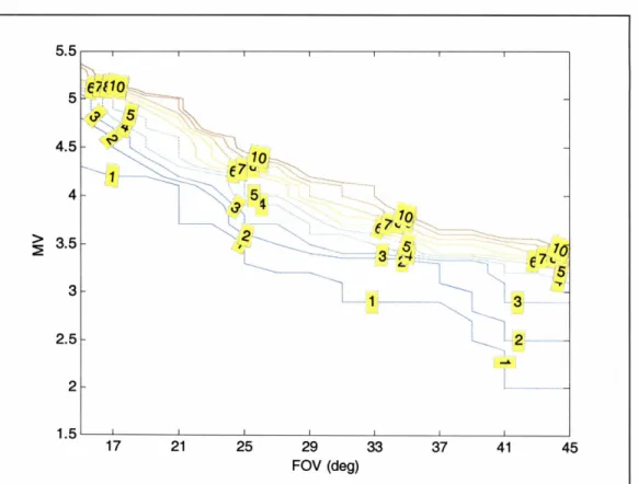
Table 5.1 Required Mv for a Given Minimum Number of Stars and FOV 89...
Table 5.2 Parameters for Mv Trade Study 91...
Table 5.3 Statistical Mv Data for 500 Stars 92 Table 5.4 Results of S Matrix Construction...
113Table 7.1 Parameter Settings for Centroider Performance Tests
...
127Table 7.2 Weighted Sum Centroider Comparison Statistics
...
132Table 8.1 Optimal Centroider Based on Speed and Accuracy Performance Results ... 166
...
a
DK
f
FF FFSR full Well lens aperture (cm)number of dark current noise electrons (electron count)
lens focal length (mm) imager fill factor (%)
product of fill factor and spectral response ( A N )
maximum number of electrons that one imager pixel can contain (electron count)
image sensor gain (electron count/ADU)
field of view in the horizontal direction (4
visual magnitude
width of Gaussian approximating the point spread function of a star (pixels)
standard deviation of the noise (electron counts)
pixel pitch in the x-direction (pm)
pixel pitch in the y-direction (pm)
quantum efficiency (%)
number of readout noise electrons (electron counts)
number of stellar electrons (electron counts)
Vi
-
-
unit vector defining the position of the im starAD ADC ADU CCD CID CMOS FAR-MST FOV GPS LIS LIST MMACS PSF SNR analog-to-digital analog-to-digital converter analog-to-digital unit charge-coupled device charge-induction device complementary metal-oxide-semiconductor
fast angular rate miniature star tracker
field of view
Global Positioning System
lost-in-space
lightweight inexpensive star tracker
Million Multiply Accumulate Cycles per Second
point spread function
Chapter 1
BACKGROUND AND MOTIVATION
1.1 Attitude Sensors for Satellites and Spacecraft
All satellites and spacecraft require onboard attitude sensors to ensure maintenance of the projected trajectory. Errors in attitude sensing andfor tracking can result in significant damage, or in the worst case, complete loss of the spacecraft. Ideal attitude sensors can function independently from other onboard systems and can report current position and rate information instantaneously. An attitude sensor is generally designed to work in conjunction with an attitude controller. Once the attitude sensor detects an undesired deviation in course heading or speed, it signals the amount of deviation and the type of correction needed to the controller; the controller is then responsible for firing thrusters or other actuators to perform the corrective maneuver to return the spacecraft to its appropriate route.
A wide variety of attitude sensors exist, but their particular characteristics depend largely on the intended application. Nonetheless, the general design objectives of all attitude sensors are the same, as displayed in Table 1.1.
Table 1.1 Attitude Sensor Goals
Unfortunately, most attitude sensors have to prioritize between their desired success rates, computational speed and storage allotments, and hardware parameters. As a result, attitude
Maximize
accuracy reliability wide-angle capture ability
number of axes that can provide information insensitivity to celestial bodies
other than the one(s) it seeks lifetime
Minimize
mass size power consumption time delay in information relay
operating limits cost
sensors that are most appropriate for one particular mission type, may be very different from attitude sensors applicable for a different mission type. However, because of the wide spread of satellite and spacecraft mission profiles in comparison to the number of attitude sensor types, individual missions are forced to rank which attitude sensor properties are most desirable and select one from those currently available.
1.2 Types of Attitude Sensors
There are numerous types of attitude sensors, but among the most popular are Earth sensors, Sun sensors, magnetometers, Global Positioning System receivers, and star trackers. Detailed below are brief introductions to these types of attitude sensors, including their respective purposes, hardware properties, and limitations.
1.2.1
Earth
Sensor
Earth sensors, also known as horizon scanners, determine spacecraft attitude relative to the Earth's horizon. They are generally used for space navigation, communication, and weather reports. Earth sensors have flown on the United States Mercury and Gemini manned spacecrafts and are currently implemented onboard various aircraft.
Earth sensors are appropriate for spacecraft and satellites within a reasonable proximity to the Earth. However, the crafts especially near the Earth can have 40% of their field of view (FOV) filled by the Earth itself, which makes it difficult to obtain accurate attitude information based on the Earth as a whole. Instead, these sensors locate the Earth's horizon and use it as a means of attitude determinati~n.''~
It has been shown that the position of Earth's horizon is the least ambiguous in the spectral region near 15pm in the infrared. The spectral region of choice for most Earth sensors is the C02 band because it has the most uniform intensity across the ~ a r t h . ' ~ ' One advantage of working in this realm is that the sensors can work just as effectively during the night as during the day and that they are naturally less susceptible to reflected light off of the craft than those sensors that work in the visible spectrum.
Earth sensors have four basic components: a scanning mechanism, an optical system, a
radiance detector, and signal processing electronics."] An Earth sensor designed by Goodrich
Corporation is displayed in Figure 1.1 .I3]
Eatth Sensor Tel.rcope
Figure 1.1 Goodrich Corporation Multi-Mission Earth Sensor Model 13-410[~'
Earth sensors do have several significant limitations. They have been known to perform
poorly when high-altitude cold clouds are present or during solar interference, especially when
close to the horizon.[41 Therefore, sufficient Sun rejection capability is a primary requirement for most Earth sensors. Additionally, uncertainties in temperature and altitude of the sensor are two other common sources of error.
1.2.2
Sun
Sensor
Sun sensors are similar to Earth sensors, except they provide attitude information relative to the Sun, as opposed to the Earth. Apart from attitude determination, they are also used to protect delicate onboard equipment and position solar power arrays.['] Solar sensors hold the advantage over Earth sensors in that the angular radius of the Sun is nearly Earth-orbit
independent and small enough that for most missions a point-source approximation can be
1
There are three primary categories of Sun sensors: analog sensors, Sun presence sensors,
and digital sensors. Due to the fact that Sun sensors are used in a wide range of applications, their fields of view (FOVs) range from several arc-minutes to a full 360". An important advantage of Sun sensors is that they generally require no onboard power systems because their
satellites or spacecraft use the Sun as their power source. Figure 1.2 shows an example of four medium Sun sensors surrounding a coarse Sun sensor designed by AeroAstro, In~orporated.~~]
Figure 1.2 AeroAstro, Incorporation Medium and Coarse Sun sensors"
The primary disadvantage of solar sensors is that satellites and spacecraft implementing
them must continuously be concerned with the orientation and time evolution of the Sun vector
in the body coordinate frame. In other words, the Sun must always remain in the FOV for the
attitude sensor to be useful. This can pose strong limitations on mission flexibility. Another disadvantage is due to the natural occurrence of solar aging, which is caused by the persistent exposure to solar ultraviolet radiation. This can only be reduced through radiation shields and
light baffles, which increase the mass requirements of the sensor.
1.2.3 Magnetometers
Magnetometers are vector sensors that measure the orientation of satellites and spacecraft relative to a particular magnetic field, usually that of the Earth. These sensors run alternating currents through three mutually perpendicular coil-wound rods to magnetize the rods. The current is applied in one direction, and then in the opposite direction, and the orientation of the rods relative to the Earth's magnetic field is indicated by an imbalance in the alternating current output from the coils with respect to zero voltage.'"
Magnetometers have two components: a magnetic sensor and an electronics unit that transforms the sensor measurements into a useable format.[71 Figure 1.3'~' depicts a
magnetometer in use aboard the Voyager spacecraft, which studied the outer planets of Jupiter,
Saturn, Uranus, and Neptune in the 1970s and 1980s.
Figure 1 3 Voyager Spacecraft with Magnetometer Boom ~xtended'~'
There are several significant limitations to magnetometers. First, due to the nature of how the rods are used to determine orientation, magnetometers can only determine attitude infomation about two axes; an additional sensor is necessary to obtain information about the
third axis. Second, the use of the Earth's magnetic field becomes problematic because it is not completely known, and the models used to predict its magnitude and direction at the satellite or spacecraft's location are subject to substantial errors.'71 Additionally, because the Earth's magnetic field strength decreases with distance from the Earth as 112, magnetometers are generally limited to operate below an altitude of 1000krn.; above this altitude, residual craft magnetic biases tend to dominate the total magnetic field measurement."'
1.2.4
Global
Positioning
System
Receivers
The Global Positioning System (GPS) is a constellation of 27 Earth-orbiting satellites, 24 active and 3 spares, that was first designed and implemented by the United States Air Force in
55" with right ascension of the ascending nodes separated by 60°, as shown in Figure 1.4[99101 These orbits are aligned so that at least 4 satellites are always within the line of sight from nearly any location on the Earth.
Figure 1.4 GPS Satellite ~ o n f i ~ u r a t i o n ~ ~ ~ '
GPS receivers are attitude sensors that calculate their current position, which includes latitude, longitude, and elevation, as well as the precise time aboard the satellites. The objective of a GPS receiver is to locate 4 of the GPS satellites, determine the distances to each, and then deduce its own location; this is accomplished using the mathematical principle known as trilateration, which is the process of determining relative positions of objects using the geometry of triangles.'' l1 GPS receivers contain the following components/functions: antenna, preamplifier, reference oscillator, frequency synthesizer, downconverter, intermediate frequency (IF) section, signal processing, and navigation processing, as displayed in Figure 1.5.'~~ These elements work together to acquire signals from the satellites, filter noise and interference, and finally output the receiver's position.
PROCESSING
VELOCITY. nME. ETC
REFERENCE FREQUENCY OSCILUTOR
Figure 1.5 GPS Receiver Block ~ia~rarn"'
Although GPS receivers have the potential for producing highly accurate positioning estimates, there are several disadvantages to using them. One of the largest contributors to receiver inaccuracies results from changing atmospheric conditions. Varying conditions unpredictably alter the speed of the GPS signals as they pass through the Earth's ionosphere, which is the atmospheric layer ionized by solar radiation.[12] The only means of alleviating this is to wait until satellites are more directly overhead, where the signal travels through less distance of the ionosphere. Signals can also be degraded because of multi-path reflections of the radio signals off of the ground or surrounding structures such as buildings or mountains.[121 With regards to spacecraft attitude sensing, current GPS receivers are limited in that they are currently restricted for use below altitudes of approximately 10,000krn.
1.2.5 Star Trackers
Star trackers are composed of three elements: an optics system that incorporates a pinhole, single, or double lens that enables the capture of stellar photons, a detector system generally composed of a charge-coupled device (CCD), charge-injection device (CID), or complementary metal oxide semiconductor (CMOS) onto which the star light is defocused, and an electronics processing unit that both digitizes and analyzes the stellar data. Star trackers measure stellar coordinates and compare them to known coordinates from either an onboard star catalog or from previous images. This comparison results in attitude information within the star tracker body frame, which can then be translated into the spacecraft body frame or to an inertial reference frame. In general, star trackers are the most accurate attitude sensors because they have the potential of achieving accuracies within several arc-seconds. Also, since they do not
rely on the positions of the Earth, Sun, magnetic fields, or external satellites, they are highly flexible attitude sensors.
The earliest star trackers required initial, coarse attitude estimates from other onboard attitude sensors. In the 1940s and early 1950s, star trackers were used in aircraft and missile guidance to provide celestial reference for position and bearing determination that was available during the day and night.[13' In the 1950s and 1960s, star trackers were used in conjunction with gyro-stabilizing platforms to more accurately align rockets prior to launch. Star trackers continue to be used in the stabilization of Earth-orbiting, Lunar, and planetary satellites and spacecraft. Fortunately, with increasing duration and more complicated mission requirements, solid state imaging devices, such as the CCD, CID, and CMOS imagers, have been incorporated, which have drastically improved reliability and attitude information accuracy.
There are three types of star trackers: star scanners, which use the craft's rotation to dictate the searching and scanning function, gimbaled star trackers, which search for and acquire stars via mechanical movement, and fixed head star trackers, which electronically search for and track stars over limited ~ 0 ~ s . ~ ' ~ A star scanner was used onboard the Galileo spacecraft, in addition to Sun sensors and gyroscopes, to provide the most accurate and final attitude.[15] This is highlighted in Figure 1.6 by the red arrow.
Figure 1.6 Star Scanner Example
-
GPlileoacecr craft'^^^
The United States Air Force SR-71 Blackbird, RC-135 Rivet Joint surveillance aircraft, and the B-2 Spirit, displayed in Figure 1.7'~~. '*I, all implement gimbaled star trackers.[19' In the B-2, the star tracker observations are made through a 7in window located in the left wing.
Figure 1.7 Gimbaled Star Tracker Example; Top Left - SR-71, Top Right - RC-135, Bottom
-
B-2""'''
The Astro-1 observatory aboard STS-35, depicted in Figure 1.8, relied on a fixed head star tracker (FHST).'~~] The FHST was supposed to acquire, track, and identify stars of known visual magnitude, but the star tracker erroneously calculated the visual magnitudes to be lower than what they were in reality, severely hampering the outcome of theAs evident in these examples, star trackers have been implemented onboard some of the most sophisticated aircraft, spacecraft, and satellites that have accomplished impressive feats.
Star trackers were selected as the primary attitude sensors in these missions because of their potential for high sensing and tracking accuracy. The unfortunate tradeoff for high precision is significant increases in mass, computational expense, and power consumption. Regardless, all of
these missions were multi-million dollar ventures where the most advanced attitude sensors were not only appropriate, but were crucial, and so these tradeoffs were relatively inconsequential.
However, there are numerous current missions, many of which have a high potential for significant scientific advancement, that cannot afford the large increases in mass, computational expense or power consumption. Whether these missions emanate from small start-up companies or large government proposals, their objectives remain high. The pervasive requirement to drive down overall weight and volume of satellites and spacecraft in order to minimize propulsive expenses for launch will require attitude sensors that are small enough to accompany their reduced hardware sizes, while simultaneously maintaining their effectiveness in attitude determination. The second through fifth rows of Table 1.2 describe the five attitude sensors discussed above. It is clear from this table that current star trackers can perform under the most variable operating conditions and can provide the most accurate attitude information, but these advantages come at the expense of requiring the greatest size, mass, power consumption, and
cost.
Table 1.2 Comparison of Current Attitude Sensors
Sensor Earth Sensor Sun Sensor Magnetometer Available GPS Num. Axes 2 Operating Angular Range Narrow: Nadir A -1 0" Narmw: Sun i -30" None in eclipse Full sphere, but need
magnetic clean sat.
Obits Circ., small alt. range Any LEO only SlzelMass/ PowerlCost Medium Low Low Accuracy1 Angular Rate Medium/ High Low1 High Low/ High
The majority of missions are not at the same level as those of Galileo or Astro-1, and so a new method of attitude sensing that can provide low cost, high performance micro-satellites with appropriate means of attitude determination is currently desirable. This goal is best described by Junkins (2003):
"In order to accelerate the evolution of faster, better, cheaper spacecraft, it is evident that greatly enhanced general-purpose attitude determination methods are needed. There is a clear need for lightweight, accurate, reliable, and inexpensive systems for spacecraft attitude estimation. Moreover, the use of smaller satellites have more onboard processing as well as reduced ground computer support has encouraged the development of lightweight, autonomous star trackers. Such star trackers should be able to identify and track star patterns in arbitrary directions without prior information, additional sensor support, or ground processing. ,,[13]
To meet these requirements, new opportunity "micro" star trackers are currently being designed with properties specified in the final row of Table 1.2. These star trackers hope to provide medium to high attitude sensing and tracking accuracies in all three axes, while simultaneously minimizing their own size, mass, power consumption, and cost. Several existing micro star trackers include the Jet Propulsion Laboratory's ASTROS star tracker, Ball Aerospace's CT-600 series star trackers, Lockheed Martin's Coming OCA improvement to the Lawrence Livermore National Laboratory Clementine star tracker, and Junkin's DIGISTAR star tracker. Two specific star trackers, which are the focus of this paper, are described briefly below.
1.3 The Next Generation of Star Trackers
Two next-generation star trackers, the Lightweight Inexpensive Star Tracker (LIST) and the Fast Angular Rate Miniature Star Tracker (FAR-MST), are currently under joint development by AeroAstro, Inc. and the Massachusetts Institute of Technology Space Systems Laboratory. The purpose of LIST and FAR-MST is to provide star tracker position and rate determination to small, highly maneuverable, low-cost spacecraft. Thus, LIST and FAR-MST propose a better balance between attitude determination accuracy and cost metrics, providing more affordable attitude sensors to smaller vehicles.
LIST and FAR-MST star trackers differ with respect to their attitude performance abilities, as described in Figure 1.9.'~~' LIST is a simpler, minimum requirement star tracker capable of determining relative rate information. FAR-MST can achieve rate information during faster tumbles and also will provide lost-in-space (LIS) capability, by determining spacecraft orientation without prior attitude information
[stars patterns are (stars streak are
compared against examined to
eterrnine rate
- - - . I - - I I I
Tkacking Hods (relative motion sf
Figure 1.9 Comparison of LIST and FAR-MST Attitude ~etermination'~~'
To meet physical requirements, appropriate constraints on optics, memory, and computational speed have been defined and included in the hardware selection and software design. The targeted hardware characteristics of FAR-MST include a mass below lkg, dimensions smaller than 15cm x 8cm x 8cm, power consumption not exceeding 3W, and cost less than $look, as shown in Table 1.3. [239 241 Since LIST has more lenient rate sensing requirements, the targeted characteristics for LIST are somewhat smaller than those for FAR- MST.
Table 1.3 LIST and FAR-MST Operational G o a p u '
Despite their restrictive specifications, LIST and FAR-MST star trackers will still be capable of performing attitude determination at 1Hz update rate with an accuracy of 100arcsec. LIST and FAR-MST will manage tumble rates up to 1'1s and 10°/s, respectively.
dimensions (cm3) mass (kg)
power consumtion (W)
cost ($k)
limiting MV
stars tracked per fiame pitch/yaw accuracy (arcsec) roll accuracy (arcsec) max acquire rate (Ols) max sensing rate ("Is) max tracking rate (Vs) update rate (Hz)
FOV (O)
onboard star catalog (# stars) supporting satellite weight (kg) mode of operation
The primary software algorithms include functions to extract and centroid stars from image noise and to match star patterns between subsequent images or to a small on-board catalog. The current algorithms incorporate various ideas from open literature, but appropriate modifications and improvements have been made where applicable. Thresholding at low signal- to-noise is accomplished using a statistical pre-filter to address high noise content. Centroiding examines the stellar shape to optimally set shutter time at different rotation rates. Pattern matching between frames implements a 'smart' star selection technique to avoid wasted time on stars that might not appear in both images. Several algorithms, including the pair match, triangle match, and rate match, are used for frame-to-frame matching. Additionally, an n-vertex pattern match can be performed against a star catalog that has been reduced either based on the probability that the stars would be used or by existing attitude information. This variety in pattern matching algorithms enables the codes to be implemented in a dynamic manner based on
LIST 5.1 x 7.6 x 7.6 0.3 < 1 4 < 4 70 1080 1 30 none tens to hundreds relative tracking FAR-MST 1 5 x 8 ~ 8 0.9 3 100 4.5 I > 2 100 4 15
.
10 25 to 45 < 500 LISthe number of stars present in the image and whether or not current rate information is available. This provides several modes of operation and graceful degradation of performance at higher angular rates. Finally, a recursive estimation technique is used to generate attitude quaternion solutions from the pattern matching results.
The principle goal of next-generation star trackers, such as LIST and FAR-MST, is to provide micro-satellites and spacecraft with accurate attitude information without the lofty mass, size, power consumption, and cost requirements that constrain most current star trackers. These goals are accomplished by selecting particular hardware components that are capable of meeting star tracker needs. Table 2.1 compares the FAR-MST star tracker with current star trackers designed by Goodrich, Ball Aerospace, SODERN, and Galileo. [25,26,27,28,29]
Table 2.1 Comparison of Existing Star Trackers and FAR-MST Star Tracker W"n3a291
Star trackers are composed of three main hardware elements: optics, imager, and processor. The optics subsystem is used to collect and focus light onto the image plane. The
imager digitizes the photons into electrons and passes them to the processor, which converts digitized electron signals into quantities that can be used in the pattern matching and attitude defining algorithms. These subsystems are assembled together in a manner similar to that shown
below for the ASTROS star tracker in Figure 2.1.[301 The sensor assembly receives incoming
light rays through a single lens, projects the photons onto the CCD, and generates the
corresponding digital star-image pixel data. The electronics assembly receives the digitized data Star Tracker Sire (an) Mass (kg) Power (W) Cost (Sk) Accuracy (srcaac 3a) Max Acquire Rate ("lsec) Max Tracking Rate ("lsec)
.
Max Sensing Rate ["fsec) Ball CT-633 3 4 x 1 9 ~ 1 9 2.85 10 > 600 40 0.2 10 None Goodrich HD-1003 4 1 x 1 6 ~ 1 1 3.54 10 550 25 0.8 1.4 None SODERN SED-16 2 9 x 1 7 ~ 1 6 3.0 12.8 > 500 70 7.0 20 None Gsiiw AA-STR 1 8 x 1 2 ~ 1 2 1.1 3.8 -300 98 1 .O Ae&tro FAR-MST 1 5 x 8 ~ 8 0.9 3 100 100 4.0 NIA 10 4 10I
and uses the processor and memory to run the image processing algorithms necessary for attitude determination.
SENSOR ASSEMBLY I
I ELECTRONICS ASS€ MBLY
(SAl I E A I I VACUUM I INTERFACE
-
IMAGE MOTION COMPENSATION IIMCI SYSTEMFigure 2.1 ASTROS Tracker Block ~ia~rarn'"]
Figure 2.2 shows a simple schematic of how the hardware functions en bloc to produce attitude information for the satellite.r291 Stellar light rays enter the optics system and are focused on the imager. The processor then uses the image, pattern recognition software, and onboard star catalog to output the roll, pitch, and yaw position as attitude information.
Roll,
Pitch, and
Yaw
Position
( ~Y.
9 z)Figure 2.2 LIST and FAR-MST Star Tracker Block Diagram ["I
2.1
Processor
Selection
A star tracker processor is used to convert the image stored by the sensor into information
useful to the software that eventually outputs attitude information. The parameters of importance for LIST and FAR-MST star trackers are clock speed and power consumption. Several processors have been considered, including the Hitachi SH7065 processor and Analog Devices, Inc.'s Blackfin ADSP-BF533. The Blackfin BF533 has been selected for FAR-MST and its parameters of importance are displayed in Table 2.2.1311
Table 2.2 Blackfin ADSP-BF533 ~ r o ~ e r t i e p ' '
max clock speed (MHz)
max MMACS
,RAM (kBYtes)
external memory bus (# bit) core voltage (V) 750 1500 148 16 0.8 to 1.26
2.2 Imager Selection
Star tracker imagers are responsible for the digital conversion of the photons collected by the lens into electrons that can be read by the processing unit. Current star trackers generally implement either charge-injection devices (CIDs), charge coupled devices (CCDs), or complementary metal oxide semiconductors (CMOS) detectors. The primary difference between these three types of imagers is the variation in signal readout methods, as is explained below.
2.2.1 CID Imagers
General Electric Company initiated the concept of charge-injection devices (CIDs). In 1972, General Electric's scientists used the photosensitive properties of silicon to develop a simple array of photosensitive capacitor elements, which eventually evolved into the first CID camera. Since the 1970s, CIDs have evolved to provide high resolution with blooming resistance, broad spectral response capabilities, and asynchronous operation modes for detection and measurement.
CIDs are composed of a two-dimensional array of charge-coupled MOS storage capacitors. They measure signal charge in
sit^'^^],
meaning electron charges are not removed from the original pixels during readout. Although this type of reading is difficult, the charge remains intact following readout, thus preventing the data from being erased. Signal reading is generally accomplished by "sequential-injection" or "parallel-injection."[331 When a clear pixel map is desired for a new image, electrodes in each pixel are temporarily switched to ground, "injecting" the charge into the silicon.[341Because of this unique data-readout process, CID imagers hold several important technical advantages over other imaging devices. CCDs and CMOS detectors suffer from low fill factors. However, since CIDs have a contiguous pixel structure, their fill factors are always loo%, which translates to higher image resolution. Because the readout process is nondestructive, CIDs have large degrees of exposure control. This means that low-light static images can be captured, and images can be exposed for long time periods, until an optimal exposure develops.[341 Solid state imaging, such as that provided by CCDs, is often challenged
by pixels "blooming" and "smearing," caused by individual pixels reaching their maximum fullwell saturation levels and spilling their electrons into adjacent pixels during longer exposures at the brighter intensity levels. However, CIDs better tolerate bright intensity levels because electrons are confined to the pixels in which they were originally placed, since charge does not move from pixel to pixel in these imagers.
CIDs can implement several different types of progressive scanning modes. When the fastest capture rate is desired over full resolution, the image frame can be downsized. Also, particular regions of the FOV can be isolated to more quickly update specific windows of interest to the user. CIDs also have the ability to act in a "freeze-frame" mode to enable images to be viewed for shorter or longer periods of time?]
2.2.2 CCD
Imagers
The charge-coupled device (CCD) was first developed by Willard Boyle and George Smith at AT&T Bell Labs in 1969. Further advances in CCD technology were made by Fairchild Semiconductor, RCA, and Texas Instruments, and the first commercial device was manufactured in 1974 by Fairchild Semiconductor. CCDs are known for their fast speed, high dynamic range, low noise, and excellent resolution capabilities. However, the primary disadvantage of CCD imagers is their high power consumption.
A charge-coupled device is composed of an array of photosensitive coupled capacitors embedded in an integrated circuit, where each capacitor, or pixel, accumulates and stores electric charge. Prior to digitization, charge must be moved from the original pixel locations to the end columns in their row where they are sent through an analog-to-digital converter (ADC) to be read. Readout times are small in comparison to integration times to prevent image smearing.
The CCD is commonly implemented in one of three different architectures: full-frame, frame-transfer, and interline.I3'] The full-frame architecture uses a mechanical shutter instead of an electronic one, and all of its image area is active. The frame-transfer architecture is more expensive than the full-frame architecture because half of the silicon area on the imager is covered by an opaque mask. This opaque area provides an additional storage area for readout
while a new image can be simultaneously integrated in the active area. The primary disadvantage of a full-frame CCD is the increased power requirements of the mechanical shutter. The interline architecture covers every-other column of the imager with the opaque mask. This architecture is advantageous because it only requires charge to move one pixel over to reach a storage and readout region. The unfortunate tradeoff is that the overall fill factor and quantum efficiency are decreased to 50%. Modifications have been made to the interline architecture to improve the imager's fill factor by incorporating micro-lenses to direct light away from the opaque areas and focus it onto the active ones. In general, applications requiring maximum light capture, regardless of cost, power or processing time, should implement full-frame CCDs. However, applications requiring lower costs and lower power consumption should utilize interline CCDS.'~~]
2.2.3 CMOS Imagers
Complementary metal-oxide-semiconductor (CMOS) circuits were developed by Frank Wanlass at Fairchild Semiconductor in 1963. CMOS imagers read image data through the use of transistors, located at each pixel, that amplify and transfer the charge. In terms of the reading process, CMOS imagers are more flexible than CCD imagers because each pixel in a CMOS imager can be individually read.1361 This enables a window-of-interest, or "windowing," capability that is useful in image compression, motion detection, and target tracking.[371
There are two types of CMOS imagers: ones with passive pixel sensors and ones with active pixel sensors. Passive pixel sensors are the oldest CMOS imagers and were first used in the 1960s. Photosites convert photons into electrical charges. The main drawback of passive pixel sensors is that high background noise is generated in the image. Active pixel sensors were designed to reduce the noise associated with passive pixel sensors. This is accomplished by implementing "active circuitry" to determine and cancel out the noise level at each pixel. Active pixel sensors allow for larger image arrays and enable higher resolution due to this noise cancellation ability while still consuming considerably less power than CCDs.
In general, the first CMOS imagers were prone to lower resolution and lower sensitivity in comparison to other solid state imagers. However, significant improvement has been made to
bring them almost up to par with CCD imagers. Although CMOS imagers still do not provide quite as much accuracy and flexibility as CCD imagers, CMOS imagers are significantly less expensive and are beginning to show capabilities comparable to CCD imagers.
One of the largest problems with CCDs is the fact that their hardware characteristics require them to be manufactured using specialized and expensive processes, which are used exclusively for CCD production.[381 However, CMOS imagers use the same processes and equipment as computer processing and memory chips, which are mass-produced all over the world. This standard fabrication ability is the foremost reason CMOS imagers are much less expensive than CCD imagers.
There are two disadvantages of CMOS detectors. First, CMOS chips have fill factors lower than CCDs, making them less sensitive to light and therefore requiring longer exposure times to capture the same number of photons. Second, they have higher noise levels than CCDs, requiring longer processing times to reduce the noise.
Despite these few shortcomings of CMOS imagers, their low cost, low power consumption, imbedded analog-to-digital (AD) conversion and amplification, and windowing capabilities make them the imager of choice for micro star trackers like LIST and FAR-MST. Table 2.3 compares six different CMOS detectors manufactured by three different companies.
Table 2.3 Comparison of Various CMOS ~ m a ~ e r s ' ~ ~ ' "' 41' 4 2 433 "I
The imager selected for LIST and FAR-MST is Fillfactory ' s IBIS5-A- 1300, which is displayed in Figure 2.3. This imager was chosen because of its low power consumption, high sensitivity, fast frame rate and large QE, as shown in Table 2.3.
active image area (mm2)
active array format
(# pixels) pixel size (pm2) frame rate (fps) shutter mode ADC conversion gain ( pvle') FF (%) FFSR (AIW) QE (%I peak QE
*
FF (%) sensitivity (VILx-s) fullwell (# e? dynamic range (dB) dark current . ( p ~ / c m 2 )dark current rate
(# of e'/s) power dissipation (mW) operating ,temperature ("C) KAC-9638 6.27 x 7.81 1288 x 1032 6 x 6 18 rolling reset 8 and 10 bit 49 57 150 -10 to +50 Kodak KAC-01301 3.47 x 2.78 1284x 1028 2.7 x 2.7 16 continuous, single frame rolling 10 bit TBD TBD 49 < 100 -30 to +70 MT9M001 6.66 x 5.32 1280x 1024 5.2 x 5.2 30 electronic rolling 10 bit < 15 c 55 2.1 68.2 363 0 to 70 Micron MT9M413 15'36 12.29 1280x 1024 12 x 12 < 500 trueSNAP freeze-frame 10 bit 13 40 < 25 1600 bits/ Lx-s 63000 59 50 mV/s < 500 at 500 fps, < 150 at 60 fps -5 to +60 Fillfactory IBIS4-1300 1280x 1024 7 x 7 7 (on chip ADC),<23 (analog output) electronic rolling 10 bit < 16 60 0.165 > 50 > 30 7 70000 < 100 344 1055 535 IBIS5-A-1300 1280x 1024 6.7 x 6.7 <27.5 rolling, snapshot 10 bit 17.6 50 0.16 > 60 30% c 8.46 < 100 410 175 0 to 60
Figure 2.3 Fillfactory IBISS-A-1300 CMOS
2.3
Optics Design
The primary function of a lens is to collect and focus light rays. The important
parameters for consideration in imaging lenses are aperture, focal length, f-number, format, and
resolution.
A lens' aperture is its diameter. Larger apertures correspond to larger lenses, and therefore have higher light collecting capabilities. The downside of large apertures is increased mass. In general for star trackers, the largest lens that does not exceed hardware constraints is desired to maximize light collection, allowing for drnmer stars to be processed at faster rates. A
lens' focal length is the distance between the lens and the location of the focused image. Long
focal lengths correspond to high magnifications and narrow FOVs, whereas short focal lengths correspond to low magnifications and wide ~ 0 ~ s . ' ~ ~ ' The focal length and FOV of the lens and imager plane are related by
where w is the width of the imager and f is the focal length. A lens' f-number, or focal ratio, is the ratio of the lens' focal length to its aperture. Smaller f-numbers correspond to greater light collection ability while larger f-numbers correspond to greater latitude for focus.'"'
When selecting the proper star tracker optical and imaging hardware, a lens' format and
of the imager plane helps dictate the necessary size of the lens' format and vice-versa. For example, an imager having a ?4 inch optical format, which corresponds to a diagonal of approximately 4 mm, should be paired with a lens also having a ?4 inch format.[451 This ensures that the star tracker will make use of the entire imaging array, including the comers. The resolution of the lens should match the resolution of the imager, which can be measured by the number of microns contained in a single pixel. For example, an imager containing pixels that are 5 microns wide should be matched with a lens that can resolve 5 micron wide features.[451 Improperly matched optical and imaging subsystems can result in blurry images and, consequently, inaccurate attitude information.
Star trackers have the flexibility to implement several different lens types. Three lenses have been considered for LIST and FAR-MST, which include a pinhole, single lens, and double lens. Their respective properties are displayed in Table 2.4.
Table 2.4 Lens Comparison
Type I Pinhole Single Lens L Double Lens Advantages simple no additional mass no radiation yellowing
larger light gathering area -* higher light capturing ability -+ shorter exposure times required -+ lower SNR allowed
-+ higher capacity in roll direction sensor protected
larger light gathering area -* higher light capturing ability -* shorter exposure times required -* lower SNR allowed
-* higher capacity in roll direction sensor protected
removal of curvature of fields effect
Disadvantages small light gathering area
-* low light capturing ability -* longer exposure times required
-
higher SNR required-* less capacity in roll direction open to radiation
open to contaminants
additional mass required
lens radiation yellowing
curvature of fields effect
additional mass required
The pinhole was initially considered for LIST because of its simplicity and low cost. However, testing showed that the sensing and tracking capabilities did not meet the performance requirements in roll for dim visual magnitudes. The single lens does meet performance requirements, but is problematic due to the bending of the light as it passes through the lens, which results in a field curvature.
When light enters a lens, it is refracted, and all light entering perpendicular to the lens is focused to a single point, known as the lens focal point, at a distance equal to the focal length. Light entering at angles offset from the perpendicular is focused to a point also at a distance equal to the focal length, but due to the angle offset, this point is not in line with the image plane, as displayed in Figure 2.4. Therefore, light rays entering the lens at any angles other than perpendicular to the lens are projected onto a curved image plane. This results in defocused images on the actual flat imager. For star trackers, this means that stars appear larger or smaller, depending on where they fall on the imager, which can have serious effects on pattern matching and image processing algorithms. The two-dimensional curvature-of-fields effect is illustrated in Figure 2.4.
incoming light rzys
lens focal point
Figure 2.4 Illustration of Defocusing Effects Due to Field Curvature
A double lens system can be used to eliminate the field curvature. For example, a double Gauss lens refracts non-perpendicular light rays back by the appropriate angles so that all light is focused onto a flat image plane, which, therefore, prevents stellar distortion. This is illustrated in Figure 2.5. 1461
incoming light rays
imager plane
Figure 2.5 Implementing a Double Gauss Lens to Remove Field ~ u r v a t u r e ' ~ ~ ~
The primary constraint limiting the use of a double lens for LIST and FAR-MST star trackers is the resulting increased mass and size of the hardware system. Testing has shown that LIST star trackers can achieve their required accuracy using a single lens, and so a commercial off-the- shelf (COTS) single lens will be utilized in
LIST.
However, due to more rigid FAR-MST goals, a double lens will most likely be considered for FAR-MST star trackers.2.4
Hardware
Mounting
The processor, imager, and optics must be mounted together as a single unit to be attached to the satellite or spacecraft. The optics and imager are generally assembled using a C, S, CS, or X mount; the difference between these mounts is the number of threads and the back flange-to-image distance. An example of the imager and electronic assembly of the ASTROS star tracker is shown in Figure 2.6.[301 The ASTROS star tracker implements Texas Instrument's
Figure 2.6 ASTROS Tracker Hardware ~ s s e r n b l ~ ' ~ '
Once the star tracker is assembled, it must be mounted onto the star tracker. The mount for the LIST star tracker is outlined in Figure 2.7.[471 The overall dimensions of the mount are 10.2cm x 8.9cm x 5.3cm.
Chapter
3
STELLAR SIGNAL AND NOISE
In the subsequent algorithms described in Chapters 4,5, and 6, several assumptions have been made regarding stellar signal and noise variations. The signal itself is assumed to be modeled by a two dimensional Gaussian. The stellar shot, dark current, and readout noise variations are significant electron contributions that must be considered in the image processing. Properties of the stellar signal and noise electrons are defined and discussed in this section.
3.1 Stellar Signal
As light is gathered by the star tracker, the optics system defocuses the photons on the detector. Each star that falls on the detector maps out a two-dimensional Airy function, as displayed in Figure 3 . 1 ' ~ ~ ' and Figure 3.2.["] The central portion of the Airy pattern, which is known as the Airy Disk, comprises approximately 86% of the total number of electrons that make up the star.
I
Radius at Image PlaneI
Figure 3.2 Airy Disk with Outer Rings Digitally Enhanced to Make More Easily
The Airy function, Ai(z), is defined asf501
For real values, the Airy function is written asf5']
The two-dimensional Airy function is fairly accurately approximated out to the first zero by the two-dimensional Gaussian function. The Gaussian shape is assumed to approximate the number of photons that fall on the imager. The two-dimensional Gaussian is defined asfs2]
where x and y are pixel coordinates, pi is the mean centroid location, and ci is the standard deviation from the mean. A plot of the two-dimensional Gaussian function, having bivariate normal distribution with a mean of 0 and a variance of 1, is shown below in Figure 3.3.
Figure 3.3 Gaussian Function with Bivariate Normal Distribution
On star trackers, the stellar signal is the entity that is to be measured. In the case of
CMOS and
CCD
imagers, this signal is generally measured in terms of the number of electronsthat are generated on the imager. The number of electrons, eNum, for a given star is given as
where a is the lens area, FFSR is the product of the fill factor and the spectral response of the imager, t s b , is the length of time in which the shutter is open to collect stellar light, g is the gain of the imager measured by the number of electrons represented by each analog-to-digital unit (ADU), and
M V
is the visual magnitude. The fill factor is the percentage of an individual pixel that is photo-responsive, and the spectral response is the average value of the responsiveness of the imaging element to the characteristic spectrum in units of AAV.3.2 Noise Variations
Ideally, the only photons passed through the imager are those from the stellar signal. However, all imagers contain uncertainties caused by the injection of various types of noise that are digitized along with the actual image. The most common of these are signal shot, dark current, and background noises. Additionally, there are pseudo-noise sources introduced during the process of digitizing the stellar signal, which include readout and quantization noises.
To fully comprehend digital signal and noise processing, several fundamental aspects of probability theory and statistics are required. Recall the generic formulas for one dimensional (ID) Gaussian and Poisson distributions. A 1D Gaussian distribution is modeled by
where x is a random variable, p is the mean, 0 is the standard deviation, and c? is the variance. A 1D Poisson Distribution is modeled by
where x is a random variable and A is both the mean and variance.
If XI has Poisson distribution with parameter Li, then Xl