Shapes and
Geometries
design and control and their applications. Topics of interest include shape optimization, multidisciplinary design, trajectory optimization, feedback, and optimal control. The series focuses on the mathematical and computational aspects of engineering design and control that are usable in a wide variety of scientific and engineering disciplines.
Editor-in-Chief
Ralph C. Smith, North Carolina State University Editorial Board
Athanasios C. Antoulas, Rice University Siva Banda, Air Force Research Laboratory Belinda A. Batten, Oregon State University John Betts, The Boeing Company (retired)
Stephen L. Campbell, North Carolina State University Michel C. Delfour, University of Montreal
Max D. Gunzburger, Florida State University J. William Helton, University of California, San Diego Arthur J. Krener, University of California, Davis Kirsten Morris, University of Waterloo
Richard Murray, California Institute of Technology Ekkehard Sachs, University of Trier
Series Volumes
Delfour, M. C. and Zolésio, J.-P., Shapes and Geometries: Metrics, Analysis, Differential Calculus, and
Optimization, Second Edition
Hovakimyan, Naira and Cao, Chengyu, L1 Adaptive Control Theory: Guaranteed Robustness with Fast Adaptation
Speyer, Jason L. and Jacobson, David H., Primer on Optimal Control Theory
Betts, John T., Practical Methods for Optimal Control and Estimation Using Nonlinear Programming, Second
Edition
Shima, Tal and Rasmussen, Steven, eds., UAV Cooperative Decision and Control: Challenges and Practical
Approaches
Speyer, Jason L. and Chung, Walter H., Stochastic Processes, Estimation, and Control
Krstic, Miroslav and Smyshlyaev, Andrey, Boundary Control of PDEs: A Course on Backstepping Designs Ito, Kazufumi and Kunisch, Karl, Lagrange Multiplier Approach to Variational Problems and Applications Xue, Dingyü, Chen, YangQuan, and Atherton, Derek P., Linear Feedback Control: Analysis and Design
with MATLAB
Hanson, Floyd B., Applied Stochastic Processes and Control for Jump-Diffusions: Modeling, Analysis, and
Computation
Michiels, Wim and Niculescu, Silviu-Iulian, Stability and Stabilization of Time-Delay Systems: An Eigenvalue-
Based Approach
Ioannou, Petros and Fidan, Barıs, Adaptive Control Tutorial
Bhaya, Amit and Kaszkurewicz, Eugenius, Control Perspectives on Numerical Algorithms and Matrix Problems Robinett III, Rush D., Wilson, David G., Eisler, G. Richard, and Hurtado, John E., Applied Dynamic Programming
for Optimization of Dynamical Systems
Huang, J., Nonlinear Output Regulation: Theory and Applications
Haslinger, J. and Mäkinen, R. A. E., Introduction to Shape Optimization: Theory, Approximation, and Computation Antoulas, Athanasios C., Approximation of Large-Scale Dynamical Systems
Gunzburger, Max D., Perspectives in Flow Control and Optimization
Delfour, M. C. and Zolésio, J.-P., Shapes and Geometries: Analysis, Differential Calculus, and Optimization Betts, John T., Practical Methods for Optimal Control Using Nonlinear Programming
El Ghaoui, Laurent and Niculescu, Silviu-Iulian, eds., Advances in Linear Matrix Inequality Methods in Control Helton, J. William and James, Matthew R., Extending H∞ Control to Nonlinear Systems: Control of Nonlinear
Systems to Achieve Performance Objectives
Society for Industrial and Applied Mathematics Philadelphia
Shapes and
Geometries
Metrics, Analysis, Differential
Calculus, and Optimization
SECOND EDITION
M. C. Delfour
Université de Montréal
Montréal, Québec
Canada
J.-P. Zolésio
National Center for Scientific Research (CNRS) and
National Institute for Research in Computer Science and Control (INRIA)
Sophia Antipolis
is a registered trademark. 10 9 8 7 6 5 4 3 2 1
All rights reserved. Printed in the United States of America. No part of this book may be reproduced, stored, or transmitted in any manner without the written permission of the publisher. For information, write to the Society for Industrial and Applied Mathematics, 3600 Market Street, 6th Floor, Philadelphia, PA 19104-2688 USA.
Trademarked names may be used in this book without the inclusion of a trademark symbol. These names are used in an editorial context only; no infringement of trademark is intended.
The research of the first author was supported by the Canada Council, which initiated the work presented in this book through a Killam Fellowship; the National Sciences and Engineering Research Council of Canada; and the FQRNT program of the Ministère de l’Éducation du Québec.
Library of Congress Cataloging-in-Publication Data
Delfour, Michel C.,
Shapes and geometries : metrics, analysis, differential calculus, and optimization / M. C. Delfour, J.-P. Zolésio. -- 2nd ed.
p. cm.
Includes bibliographical references and index. ISBN 978-0-898719-36-9 (hardcover : alk. paper) 1. Shape theory (Topology) I. Zolésio, J.-P. II. Title. QA612.7.D45 2011
514’.24--dc22
Alice, Jeanne, Jean, and Roger
Contents
List of Figures xvii Preface xix
1 Objectives and Scope of the Book . . . xix
2 Overview of the Second Edition . . . xx
3 Intended Audience . . . xxii
4 Acknowledgments . . . xxiii
1 Introduction: Examples, Background, and Perspectives 1 1 Orientation . . . 1
1.1 Geometry as a Variable . . . 1
1.2 Outline of the Introductory Chapter . . . 3
2 A Simple One-Dimensional Example . . . 3
3 Buckling of Columns . . . 4
4 Eigenvalue Problems . . . 6
5 Optimal Triangular Meshing . . . 7
6 Modeling Free Boundary Problems . . . 10
6.1 Free Interface between Two Materials . . . 11
6.2 Minimal Surfaces . . . 12
7 Design of a Thermal Diffuser . . . 13
7.1 Description of the Physical Problem . . . 13
7.2 Statement of the Problem . . . 14
7.3 Reformulation of the Problem . . . 16
7.4 Scaling of the Problem . . . 16
7.5 Design Problem . . . 17
8 Design of a Thermal Radiator . . . 18
8.1 Statement of the Problem . . . 18
8.2 Scaling of the Problem . . . 20
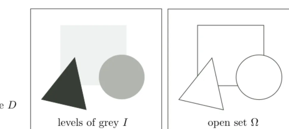
9 A Glimpse into Segmentation of Images . . . 21
9.1 Automatic Image Processing . . . 21
9.2 Image Smoothing/Filtering by Convolution and Edge Detectors 22 9.2.1 Construction of the Convolution of I . . . 23
9.2.2 Space-Frequency Uncertainty Relationship . . . 23
9.2.3 Laplacian Detector . . . 25 vii
9.3 Objective Functions Defined on the Whole Edge . . . 26
9.3.1 Eulerian Shape Semiderivative . . . 26
9.3.2 From Local to Global Conditions on the Edge . . . 27
9.4 Snakes, Geodesic Active Contours, and Level Sets . . . 28
9.4.1 Objective Functions Defined on the Contours . . . . 28
9.4.2 Snakes and Geodesic Active Contours . . . 28
9.4.3 Level Set Method . . . 29
9.4.4 Velocity Carried by the Normal . . . 30
9.4.5 Extension of the Level Set Equations . . . 31
9.5 Objective Function Defined on the Whole Image . . . 32
9.5.1 Tikhonov Regularization/Smoothing . . . 32
9.5.2 Objective Function of Mumford and Shah . . . 32
9.5.3 Relaxation of the (N − 1)-Hausdorff Measure . . . . 33
9.5.4 Relaxation to BV-, Hs-, and SBV-Functions . . . . 33
9.5.5 Cracked Sets and Density Perimeter . . . 35
10 Shapes and Geometries: Background and Perspectives . . . 36
10.1 Parametrize Geometries by Functions or Functions by Geometries? . . . 36
10.2 Shape Analysis in Mechanics and Mathematics . . . 39
10.3 Characteristic Functions: Surface Measure and Geometric Measure Theory . . . 41
10.4 Distance Functions: Smoothness, Normal, and Curvatures . . 41
10.5 Shape Optimization: Compliance Analysis and Sensitivity Analysis . . . 43
10.6 Shape Derivatives . . . 44
10.7 Shape Calculus and Tangential Differential Calculus . . . 46
10.8 Shape Analysis in This Book . . . 46
11 Shapes and Geometries: Second Edition . . . 47
11.1 Geometries Parametrized by Functions . . . 48
11.2 Functions Parametrized by Geometries . . . 50
11.3 Shape Continuity and Optimization . . . 52
11.4 Derivatives, Shape and Tangential Differential Calculuses, and Derivatives under State Constraints . . . 53
2 Classical Descriptions of Geometries and Their Properties 55 1 Introduction . . . 55
2 Notation and Definitions . . . 56
2.1 Basic Notation . . . 56
2.2 Abelian Group Structures on Subsets of a Fixed Holdall D . 56 2.2.1 First Abelian Group Structure on (P(D), △) . . . . 57
2.2.2 Second Abelian Group Structure on (P(D), ▽) . . . 58
2.3 Connected Space, Path-Connected Space, and Geodesic Distance . . . 58
2.4 Bouligand’s Contingent Cone, Dual Cone, and Normal Cone 59 2.5 Sobolev Spaces . . . 60
2.5.2 The Space Wm,p
0 (Ω) . . . 61
2.5.3 Embedding of H1 0(Ω) into H01(D) . . . 62
2.5.4 Projection Operator . . . 63
2.6 Spaces of Continuous and Differentiable Functions . . . 63
2.6.1 Continuous and Ck Functions . . . 63
2.6.2 H¨older (C0,ℓ) and Lipschitz (C0,1) Continuous Functions . . . 65
2.6.3 Embedding Theorem . . . 65
2.6.4 Identity Ck,1(Ω) = Wk+1,∞(Ω): From Convex to Path-Connected Domains via the Geodesic Distance 66 3 Sets Locally Described by an Homeomorphism or a Diffeomorphism 67 3.1 Sets of Classes Ck and Ck,ℓ . . . 67
3.2 Boundary Integral, Canonical Density, and Hausdorff Measures 70 3.2.1 Boundary Integral for Sets of Class C1 . . . 70
3.2.2 Integral on Submanifolds . . . 71
3.2.3 Hausdorff Measures . . . 72
3.3 Fundamental Forms and Principal Curvatures . . . 73
4 Sets Globally Described by the Level Sets of a Function . . . 75
5 Sets Locally Described by the Epigraph of a Function . . . 78
5.1 Local C0 Epigraphs, C0 Epigraphs, and Equi-C0 Epigraphs and the Space H of Dominating Functions . . . 79
5.2 Local Ck,ℓ-Epigraphs and H¨olderian/Lipschitzian Sets . . . . 87
5.3 Local Ck,ℓ-Epigraphs and Sets of Class Ck,ℓ . . . 89
5.4 Locally Lipschitzian Sets: Some Examples and Properties . . 92
5.4.1 Examples and Continuous Linear Extensions . . . . 92
5.4.2 Convex Sets . . . 93
5.4.3 Boundary Measure and Integral for Lipschitzian Sets 94 5.4.4 Geodesic Distance in a Domain and in Its Boundary 97 5.4.5 Nonhomogeneous Neumann and Dirichlet Problems 100 6 Sets Locally Described by a Geometric Property . . . 101
6.1 Definitions and Main Results . . . 102
6.2 Equivalence of Geometric Segment and C0 Epigraph Properties . . . 104
6.3 Equivalence of the Uniform Fat Segment and the Equi-C0 Epigraph Properties . . . 109
6.4 Uniform Cone/Cusp Properties and H¨olderian/Lipschitzian Sets . . . 113
6.4.1 Uniform Cone Property and Lipschitzian Sets . . . 114
6.4.2 Uniform Cusp Property and H¨olderian Sets . . . 115
6.5 Hausdorff Measure and Dimension of the Boundary . . . 116
3 Courant Metrics on Images of a Set 123 1 Introduction . . . 123
2 Generic Constructions of Micheletti . . . 124
2.1 Space F(Θ) of Transformations of RN . . . 124
2.2 Diffeomorphisms for B(RN, RN) and C∞ 0 (RN, RN) . . . 136
2.3 Closed Subgroups G . . . 138
2.4 Courant Metric on the Quotient Group F(Θ)/G . . . 140
2.5 Assumptions for Bk(RN, RN), Ck(RN, RN), and Ck 0(RN, RN) 143 2.5.1 Checking the Assumptions . . . 143
2.5.2 Perturbations of the Identity and Tangent Space . . 147
2.6 Assumptions for Ck,1(RN, RN) and Ck,1 0 (RN, RN) . . . 149
2.6.1 Checking the Assumptions . . . 149
2.6.2 Perturbations of the Identity and Tangent Space . . 151
3 Generalization to All Homeomorphisms and Ck-Diffeomorphisms . . 153
4 Transformations Generated by Velocities 159 1 Introduction . . . 159
2 Metrics on Transformations Generated by Velocities . . . 161
2.1 Subgroup GΘ of Transformations Generated by Velocities . . 161
2.2 Complete Metrics on GΘ and Geodesics . . . 166
2.3 Constructions of Azencott and Trouv´e . . . 169
3 Semiderivatives via Transformations Generated by Velocities . . . . 170
3.1 Shape Function . . . 170
3.2 Gateaux and Hadamard Semiderivatives . . . 170
3.3 Examples of Families of Transformations of Domains . . . 173
3.3.1 C∞-Domains . . . 173
3.3.2 Ck-Domains . . . 175
3.3.3 Cartesian Graphs . . . 176
3.3.4 Polar Coordinates and Star-Shaped Domains . . . . 177
3.3.5 Level Sets . . . 178
4 Unconstrained Families of Domains . . . 180
4.1 Equivalence between Velocities and Transformations . . . 180
4.2 Perturbations of the Identity . . . 183
4.3 Equivalence for Special Families of Velocities . . . 185
5 Constrained Families of Domains . . . 193
5.1 Equivalence between Velocities and Transformations . . . 193
5.2 Transformation of Condition (V2D) into a Linear Constraint . . . 200
6 Continuity of Shape Functions along Velocity Flows . . . 202
5 Metrics via Characteristic Functions 209 1 Introduction . . . 209
2 Abelian Group Structure on Measurable Characteristic Functions . . 210
2.1 Group Structure on Xµ(RN) . . . 210
2.2 Measure Spaces . . . 211
2.3 Complete Metric for Characteristic Functions in Lp-Topologies . . . 212
3 Lebesgue Measurable Characteristic Functions . . . 214
3.1 Strong Topologies and C∞-Approximations . . . 214
3.2 Weak Topologies and Microstructures . . . 215
3.4 The Family of Convex Sets . . . 223
3.5 Sobolev Spaces for Measurable Domains . . . 224
4 Some Compliance Problems with Two Materials . . . 228
4.1 Transmission Problem and Compliance . . . 228
4.2 The Original Problem of C´ea and Malanowski . . . 235
4.3 Relaxation and Homogenization . . . 239
5 Buckling of Columns . . . 240
6 Caccioppoli or Finite Perimeter Sets . . . 244
6.1 Finite Perimeter Sets . . . 245
6.2 Decomposition of the Integral along Level Sets . . . 251
6.3 Domains of Class Wε,p(D), 0 ≤ ε < 1/p, p ≥ 1, and a Cascade of Complete Metric Spaces . . . 252
6.4 Compactness and Uniform Cone Property . . . 254
7 Existence for the Bernoulli Free Boundary Problem . . . 258
7.1 An Example: Elementary Modeling of the Water Wave . . . 258
7.2 Existence for a Class of Free Boundary Problems . . . 260
7.3 Weak Solutions of Some Generic Free Boundary Problems . . 262
7.3.1 Problem without Constraint . . . 262
7.3.2 Constraint on the Measure of the Domain Ω . . . . 264
7.4 Weak Existence with Surface Tension . . . 265
6 Metrics via Distance Functions 267 1 Introduction . . . 267
2 Uniform Metric Topologies . . . 268
2.1 Family of Distance Functions Cd(D) . . . 268
2.2 Pomp´eiu–Hausdorff Metric on Cd(D) . . . 269
2.3 Uniform Complementary Metric Topology and Cc d(D) . . . . 275
2.4 Families Cc d(E; D) and Cd,locc (E; D) . . . 278
3 Projection, Skeleton, Crack, and Differentiability . . . 279
4 W1,p-Metric Topology and Characteristic Functions . . . 292
4.1 Motivations and Main Properties . . . 292
4.2 Weak W1,p-Topology . . . 296
5 Sets of Bounded and Locally Bounded Curvature . . . 299
5.1 Examples . . . 301
6 Reach and Federer’s Sets of Positive Reach . . . 303
6.1 Definitions and Main Properties . . . 303
6.2 Ck-Submanifolds . . . 310
6.3 A Compact Family of Sets with Uniform Positive Reach . . . 315
7 Approximation by Dilated Sets/Tubular Neighborhoods and Critical Points . . . 316
8 Characterization of Convex Sets . . . 318
8.1 Convex Sets and Properties of dA. . . 318
8.2 Semiconvexity and BV Character of dA . . . 320
8.3 Closed Convex Hull of A and Fenchel Transform of dA . . . . 322
8.4 Families of Convex Sets Cd(D), Cdc(D), Cdc(E; D), and Cc d,loc(E; D) . . . 323
9 Compactness Theorems for Sets of Bounded Curvature . . . 324
9.1 Global Conditions in D . . . 325
9.2 Local Conditions in Tubular Neighborhoods . . . 327
7 Metrics via Oriented Distance Functions 335 1 Introduction . . . 335
2 Uniform Metric Topology . . . 337
2.1 The Family of Oriented Distance Functions Cb(D) . . . 337
2.2 Uniform Metric Topology . . . 339
3 Projection, Skeleton, Crack, and Differentiability . . . 344
4 W1,p(D)-Metric Topology and the Family Cb0(D) . . . 349
4.1 Motivations and Main Properties . . . 349
4.2 Weak W1,p-Topology . . . 352
5 Boundary of Bounded and Locally Bounded Curvature . . . 354
5.1 Examples and Limit of Tubular Norms as h Goes to Zero . . 355
6 Approximation by Dilated Sets/Tubular Neighborhoods . . . 358
7 Federer’s Sets of Positive Reach . . . 361
7.1 Approximation by Dilated Sets/Tubular Neighborhoods . . . 361
7.2 Boundaries with Positive Reach . . . 363
8 Boundary Smoothness and Smoothness of bA . . . 365
9 Sobolev or Wm,p Domains . . . 373
10 Characterization of Convex and Semiconvex Sets . . . 375
10.1 Convex Sets and Convexity of bA . . . 375
10.2 Families of Convex Sets Cb(D), Cb(E; D), and Cb,loc(E; D) . . . 379
10.3 BV Character of bAand Semiconvex Sets . . . 380
11 Compactness and Sets of Bounded Curvature . . . 381
11.1 Global Conditions on D . . . 382
11.2 Local Conditions in Tubular Neighborhoods . . . 382
12 Finite Density Perimeter and Compactness . . . 385
13 Compactness and Uniform Fat Segment Property . . . 387
13.1 Main Theorem . . . 387
13.2 Equivalent Conditions on the Local Graph Functions . . . 391
14 Compactness under the Uniform Fat Segment Property and a Bound on a Perimeter . . . 393
14.1 De Giorgi Perimeter of Caccioppoli Sets . . . 393
14.2 Finite Density Perimeter . . . 394
15 The Families of Cracked Sets . . . 394
16 A Variation of the Image Segmentation Problem of Mumford and Shah . . . 400
16.1 Problem Formulation . . . 400
16.2 Cracked Sets without the Perimeter . . . 401
16.2.1 Technical Lemmas . . . 401
16.2.2 Another Compactness Theorem . . . 402
16.2.3 Proof of Theorem 16.1 . . . 402 16.3 Existence of a Cracked Set with Minimum Density Perimeter 405
16.4 Uniform Bound or Penalization Term in the Objective
Function on the Density Perimeter . . . 407
8 Shape Continuity and Optimization 409 1 Introduction and Generic Examples . . . 409
1.1 First Generic Example . . . 411
1.2 Second Generic Example . . . 411
1.3 Third Generic Example . . . 411
1.4 Fourth Generic Example . . . 412
2 Upper Semicontinuity and Maximization of the First Eigenvalue . . 412
3 Continuity of the Transmission Problem . . . 417
4 Continuity of the Homogeneous Dirichlet Boundary Value Problem . 418 4.1 Classical, Relaxed, and Overrelaxed Problems . . . 418
4.2 Classical Dirichlet Boundary Value Problem . . . 421
4.3 Overrelaxed Dirichlet Boundary Value Problem . . . 423
4.3.1 Approximation by Transmission Problems . . . 423
4.3.2 Continuity with Respect to X(D) in the Lp(D)-Topology . . . 424
4.4 Relaxed Dirichlet Boundary Value Problem . . . 425
5 Continuity of the Homogeneous Neumann Boundary Value Problem 426 6 Elements of Capacity Theory . . . 429
6.1 Definition and Basic Properties . . . 429
6.2 Quasi-continuous Representative and H1-Functions . . . 431
6.3 Transport of Sets of Zero Capacity . . . 432
7 Crack-Free Sets and Some Applications . . . 434
7.1 Definitions and Properties . . . 434
7.2 Continuity and Optimization over L(D, r, O, λ) . . . 437
7.2.1 Continuity of the Classical Homogeneous Dirichlet Boundary Condition . . . 437
7.2.2 Minimization/Maximization of the First Eigenvalue . . . 438
8 Continuity under Capacity Constraints . . . 440
9 Compact Families Oc,r(D) and Lc,r(O, D) . . . 447
9.1 Compact Family Oc,r(D) . . . 447
9.2 Compact Family Lc,r(O, D) and Thick Set Property . . . 450
9.3 Maximizing the Eigenvalue λA(Ω) . . . 452
9.4 State Constrained Minimization Problems . . . 453
9.5 Examples with a Constraint on the Gradient . . . 454
9 Shape and Tangential Differential Calculuses 457 1 Introduction . . . 457
2 Review of Differentiation in Topological Vector Spaces . . . 458
2.1 Definitions of Semiderivatives and Derivatives . . . 458
2.2 Derivatives in Normed Vector Spaces . . . 461
2.3 Locally Lipschitz Functions . . . 465
2.5 Semiderivatives of Convex Functions . . . 467
2.6 Hadamard Semiderivative and Velocity Method . . . 469
3 First-Order Shape Semiderivatives and Derivatives . . . 471
3.1 Eulerian and Hadamard Semiderivatives . . . 471
3.2 Hadamard Semidifferentiability and Courant Metric Continuity . . . 476
3.3 Perturbations of the Identity and Gateaux and Fr´echet Derivatives . . . 476
3.4 Shape Gradient and Structure Theorem . . . 479
4 Elements of Shape Calculus . . . 482
4.1 Basic Formula for Domain Integrals . . . 482
4.2 Basic Formula for Boundary Integrals . . . 484
4.3 Examples of Shape Derivatives . . . 486
4.3.1 Volume of Ω and Surface Area of Γ . . . 486
4.3.2 H1(Ω)-Norm . . . 487
4.3.3 Normal Derivative . . . 488
5 Elements of Tangential Calculus . . . 491
5.1 Intrinsic Definition of the Tangential Gradient . . . 492
5.2 First-Order Derivatives . . . 495
5.3 Second-Order Derivatives . . . 496
5.4 A Few Useful Formulae and the Chain Rule . . . 497
5.5 The Stokes and Green Formulae . . . 498
5.6 Relation between Tangential and Covariant Derivatives . . . 498
5.7 Back to the Example of Section 4.3.3 . . . 501
6 Second-Order Semiderivative and Shape Hessian . . . 501
6.1 Second-Order Derivative of the Domain Integral . . . 502
6.2 Basic Formula for Domain Integrals . . . 504
6.3 Nonautonomous Case . . . 505
6.4 Autonomous Case . . . 510
6.5 Decomposition of d2J(Ω; V (0), W (0)) . . . 515
10 Shape Gradients under a State Equation Constraint 519 1 Introduction . . . 519
2 Min Formulation . . . 521
2.1 An Illustrative Example and a Shape Variational Principle . 521 2.2 Function Space Parametrization . . . 522
2.3 Differentiability of a Minimum with Respect to a Parameter . . . 523
2.4 Application of the Theorem . . . 526
2.5 Domain and Boundary Integral Expressions of the Shape Gradient . . . 530
3 Buckling of Columns . . . 532
4 Eigenvalue Problems . . . 535
4.1 Transport of Hk 0(Ω) by Wk,∞-Transformations of RN . . . . 536
4.2 Laplacian and Bi-Laplacian . . . 537
5 Saddle Point Formulation and Function Space Parametrization . . . 551
5.1 An Illustrative Example . . . 551
5.2 Saddle Point Formulation . . . 552
5.3 Function Space Parametrization . . . 553
5.4 Differentiability of a Saddle Point with Respect to a Parameter . . . 555
5.5 Application of the Theorem . . . 559
5.6 Domain and Boundary Expressions for the Shape Gradient . 561 6 Multipliers and Function Space Embedding . . . 562
6.1 The Nonhomogeneous Dirichlet Problem . . . 562
6.2 A Saddle Point Formulation of the State Equation . . . 563
6.3 Saddle Point Expression of the Objective Function . . . 564
6.4 Verification of the Assumptions of Theorem 5.1 . . . 566 Elements of Bibliography 571 Index of Notation 615
List of Figures
1.1 Graph of J(a). . . 4
1.2 Column of height one and cross section area A under the load ℓ. . . 5
1.3 Triangulation and basis function associated with node Mi. . . 8
1.4 Fixed domain D and its partition into Ω1and Ω2. . . 11
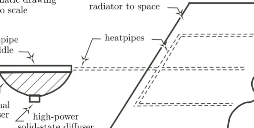
1.5 Heat spreading scheme for high-power solid-state devices. . . 14
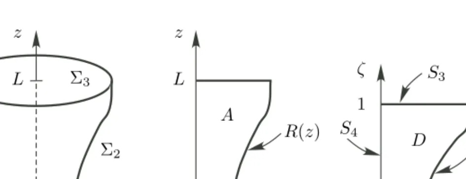
1.6 (A) Volume Ω and its boundary Σ; (B) Surface A generating Ω; (C) Surface D generating !Ω. . . 15
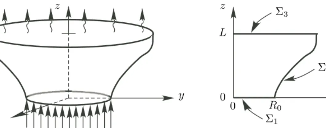
1.7 Volume Ω and its cross section. . . 19
1.8 Volume !Ω and its generating surface A. . . 20
1.9 Image I of objects and their segmentation in the frame D. . . 22
1.10 Image I containing black curves or cracks in the frame D. . . 22
1.11 Example of a two-dimensional strongly cracked set. . . 35
1.12 Example of a surface with facets associated with a ball. . . 37
2.1 Diffeomorphism gx from U(x) to B. . . 68
2.2 Local epigraph representation (N = 2). . . 79
2.3 Domain Ω0 and its image T (Ω0) spiraling around the origin. . . 91
2.4 Domain Ω0 and its image T (Ω0) zigzagging towards the origin. . . . 92
2.5 Examples of arbitrary and axially symmetrical O around the direction d = Ax(0, eN). . . 109
2.6 The cone x + AxC(λ, ω) in the direction AxeN. . . 114
2.7 Domain Ω for N = 2, 0 < α < 1, e2 = (0, 1), ρ = 1/6, λ = (1/6)α, h(θ) = θα. . . 118
2.8 f(x) = dC(x)1/2 constructed on the Cantor set C for 2k + 1 = 3. . . 119
4.1 Transport of Ω by the velocity field V . . . 171
5.1 Smiling sun Ω and expressionless sun !Ω. . . 220
5.2 Disconnected domain Ω = Ω0∪ Ω1∪ Ω2. . . 227
5.3 Fixed domain D and its partition into Ω1and Ω2. . . 228
5.4 The function f(x, y) = 56 (1 − |x| − |y|)6. . . 234
5.5 Optimal distribution and isotherms with k1 = 2 (black) and k2= 1 (white) for the problem of section 4.1. . . 235
5.6 Optimal distribution and isotherms with k1 = 2 (black) and k2= 1 (white) for the problem of C´ea and Malanowski. . . 239
5.7 The staircase. . . 248
6.1 Skeletons Sk (A), Sk (#A), and Sk (∂A) = Sk (A) ∪ Sk (#A). . . 280
6.2 Nonuniqueness of the exterior normal. . . 286
6.3 Vertical stripes of Example 4.1. . . 293
6.4 ∇dAfor Examples 5.1, 5.2, and 5.3. . . 301
6.5 Set of critical points of A. . . 318
7.1 ∇bA for Examples 5.1, 5.2, and 5.3. . . 356
7.2 W1,p-convergence of a sequence of open subsets {A n : n ≥ 1} of R2 with uniformly bounded density perimeter to a set with empty interior. . . 387
7.3 Example of a two-dimensional strongly cracked set. . . 396
7.4 The two-dimensional strongly cracked set of Figure 7.3 in an open frame D. . . 400
7.5 The two open components Ω1and Ω2 of the open domain Ω for N = 2. . . 406
Preface
1 Objectives and Scope of the Book
The objective of this book is to give a comprehensive presentation of mathematical constructions and tools that can be used to study problems where the modeling, optimization, or control variable is no longer a set of parameters or functions but the shape or the structure of a geometric object. In that context, a good analytical framework and good modeling techniques must be able to handle the occurrence of singular behaviors whenever they are compatible with the mechanics or the physics of the problems at hand. In some optimization problems, the natural intuitive notion of a geometric domain undergoes mutations into relaxed entities such as microstructures. So the objects under consideration need not be smooth open do-mains, or even sets, as long as they still makes sense mathematically.
This book covers the basic mathematical ideas, constructions, and methods that come from different fields of mathematical activities and areas of applications that have often evolved in parallel directions. The scope of research is frighteningly broad because it touches on areas that include classical geometry, modern partial dif-ferential equations, geometric measure theory, topological groups, and constrained optimization, with applications to classical mechanics of continuous media such as fluid mechanics, elasticity theory, fracture theory, modern theories of optimal de-sign, optimal location and shape of geometric objects, free and moving boundary problems, and image processing. Innovative modeling or new issues raised in some applications force a new look at the fundamentals of well-established mathematical areas such as geometry, to relax basic notions of volume, perimeter, and curvature or boundary value problems, and to find suitable relaxations of solutions. In that spirit, Henri Lebesgue was probably a pioneer when he relaxed the intuitive notion of volume to the one of measure on an equivalence class of measurable sets in 1907. He was followed in that endeavor in the early 1950s by the celebrated work of E. De Giorgi, who used the relaxed notion of perimeter defined on the class of Caccioppoli sets to solve Plateau’s problem of minimal surfaces.
The material that is pertinent to the study of geometric objects and the en-tities and functions that are defined on them would necessitate an encyclopedic investment to bring together the basic theories and their fields of applications. This objective is obviously beyond the scope of a single book and two authors. The
coverage of this book is more modest. Yet, it contains most of the important fun-damentals at this stage of evolution of this expanding field.
Even if shape analysis and optimization have undergone considerable and im-portant developments on the theoretical and numerical fronts, there are still cultural barriers between areas of applications and between theories. The whole field is ex-tremely active, and the best is yet to come with fundamental structures and tools beginning to emerge. It is hoped that this book will help to build new bridges and stimulate cross-fertilization of ideas and methods.
2 Overview of the Second Edition
The second edition is almost a new book. All chapters from the first edition have been updated and, in most cases, considerably enriched with new material. Many chapters or parts of chapters have been completely rewritten following the devel-opments in the field over the past 10 years. The book went from 9 to 10 chapters with a more elaborate sectioning of each chapter in order to produce a much more detailed table of contents. This makes it easier to find specific material.
A series of illustrative generic examples has been added right at the begin-ning of the introductory Chapter 1 to motivate the reader and illustrate the basic dilemma: parametrize geometries by functions or functions by geometries? This is followed by the big picture: a section on background and perspectives and a more detailed presentation of the second edition.
The former Chapter 2 has been split into Chapter 2 on the classical descrip-tions and properties of domains and sets and a new Chapter 3, where the important material on Courant metrics and the generic constructions of A. M. Micheletti have been reorganized and expanded. Basic definitions and material have been added and regrouped at the beginning of Chapter 2: Abelian group structure on subsets of a set, connected and path-connected spaces, function spaces, tangent and dual cones, and geodesic distance. The coverage of domains that verify some segment property and have a local epigraph representation has been considerably expanded, and Lipschitzian (graph) domains are now dealt with as a special case.
The new Chapter 3 on domains and submanifolds that are the image of a fixed set considerably expands the material of the first edition by bringing up the general assumptions behind the generic constructions of A. M. Micheletti that lead to the Courant metrics on the quotient space of families of transformations by subgroups of isometries such as identities, rotations, translations, or flips. The general results apply to a broad range of groups of transformations of the Euclidean space and to arbitrary closed subgroups. New complete metrics on the whole spaces of homeomorphisms and Ck-diffeomorphisms are also introduced to extend classical
results for transformations of compact manifolds to general unbounded closed sets and open sets that are crack-free. This material is central in classical mechanics and physics and in modern applications such as imaging and detection.
The former Chapter 7 on transformations versus flows of velocities has been moved right after the Courant metrics as Chapter 4 and considerably expanded. It now specializes the results of Chapter 3 to spaces of transformations that are
generated by the flow of a velocity field over a generic time interval. One important motivation is to introduce a notion of semiderivatives as well as a tractable criterion for continuity with respect to Courant metrics. Another motivation for the velocity point of view is the general framework of R. Azencott and A. Trouv´e starting in 1994 with applications in imaging. They construct complete metrics in relation with geodesic paths in spaces of diffeomorphisms generated by a velocity field.
The former Chapter 3 on the relaxation to measurable sets and Chapters 4 and 5 on distance and oriented distance functions have become Chapters 5, 6, and 7. Those chapters have been renamed Metrics Generated by . . . in order to emphasize one of the main thrusts of the book: the construction of complete metrics on shapes and geometries.1 Those chapters emphasize the function analytic description of sets
and domains: construction of metric topologies and characterization of compact families of sets or submanifolds in the Euclidean space. In that context, we are now dealing with equivalence classes of sets that may or may not have an invariant open or closed representative in the class. For instance, they include Lebesgue measurable sets and Federer’s sets of positive reach. Many of the classical properties of sets can be recovered from the smoothness or function analytic properties of those functions. The former Chapter 6 on optimization of shape functions has been completely rewritten and expanded as Chapter 8 on shape continuity and optimization. With meaningful metric topologies, we can now speak of continuity of a geometric objec-tive functional such as the volume, the perimeter, the mean curvature, etc., compact families of sets, and existence of optimal geometries. The chapter concentrates on continuity issues related to shape optimization problems under state equation con-straints. A special family of state constrained problems are the ones for which the objective function is defined as an infimum over a family of functions over a fixed domain or set such as the eigenvalue problems. We first characterize the continuity of the transmission problem and the upper semicontinuity of the first eigenvalue of the generalized Laplacian with respect to the domain. We then study the conti-nuity of the solution of the homogeneous Dirichlet and Neumann boundary value problems with respect to their underlying domain of definition since they require different constructions and topologies that are generic of the two types of boundary conditions even for more complex nonlinear partial differential equations. An intro-duction is also given to the concepts and results from capacity theory from which very general families of sets stable with respect to boundary conditions can be con-structed. Note that some material has been moved from one chapter to another. For instance, section 7 on the continuity of the Dirichlet boundary problem in the former Chapter 3 has been merged with the content of the former Chapter 4 in the new Chapter 8.
The former Chapters 8 and 9 have become Chapters 9 and 10. They are devoted to a modern version of the shape calculus, an introduction to the tangential differential calculus, and the shape derivatives under a state equation constraint. In Chapters 3, 5, 6, and 7, we have constructed complete metric spaces of geometries. Those spaces are nonlinear and nonconvex. However, several of them have a group
1This is in line with current trends in the literature such as in the work of the 2009 Abel Prize
winner M. Gromov [1] and its applications in imaging by G. Sapiro [1] and F. M´emoli and G. Sapiro [1] to identify objects up to an isometry.
structure and, in some cases, it is possible to construct C1-paths in the group
from velocity fields. This leads to the notion of Eulerian semiderivative that is somehow the analogue of a derivative on a smooth manifold. In fact, two types of semiderivatives are of interest: the weaker Gateaux style semiderivative and the stronger Hadamard style semiderivative. In the latter case, the classical chain rule is still available even for nondifferentiable functions. In order to prepare the ground for shape derivatives, an enriched self-contained review of the pertinent material on semiderivatives and derivatives in topological vector spaces is provided.
The important Chapter 10 concentrates on two generic examples often encoun-tered in shape optimization. The first one is associated with the so-called compliance problems, where the shape functional is itself the minimum of a domain-dependent energy functional. The special feature of such functionals is that the adjoint state coincides with the state. This obviously leads to considerable simplifications in the analysis. In that case, it will be shown that theorems on the differentiability of the minimum of a functional with respect to a real parameter readily give explicit expressions of the Eulerian semiderivative even when the minimizer is not unique. The second one will deal with shape functionals that can be expressed as the saddle point of some appropriate Lagrangian. As in the first example, theorems on the differentiability of the saddle point of a functional with respect to a real parameter readily give explicit expressions of the Eulerian semiderivative even when the so-lution of the saddle point equations is not unique. Avoiding the differentiation of the state equation with respect to the domain is particularly advantageous in shape problems.
3 Intended Audience
The targeted audience is applied mathematicians and advanced engineers and sci-entists, but the book is also suitable for a broader audience of mathematicians as a relatively well-structured initiation to shape analysis and calculus techniques. Some of the chapters are fairly self-contained and of independent interest. They can be used as lecture notes for a mini-course. The material at the beginning of each chapter is accessible to a broad audience, while the latter sections may sometimes require more mathematical maturity. Thus the book can be used as a graduate text as well as a reference book. It complements existing books that emphasize specific mechanical or engineering applications or numerical methods. It can be considered a companion to the book of J. Soko!lowski and J.-P. Zol´esio [9], Introduction to Shape Optimization, published in 1992.
Earlier versions of parts of this book have been used as lecture notes in grad-uate courses at the Universit´e de Montr´eal in 1986–1987, 1993–1994, 1995–1996, and 1997–1998 and at international meetings, workshops, or schools: S´eminaire de Math´ematiques Sup´erieures on Shape Optimization and Free Boundaries (Montr´eal, Canada, June 25 to July 13, 1990), short course on Shape Sensitivity Analysis (K´enitra, Morocco, December 1993), course of the COMETT MATARI European Program on Shape Optimization and Mutational Equations (Sophia-Antipolis, France, September 27 to October 1, 1993), CRM Summer School on Boundaries,
Interfaces and Transitions (Banff, Canada, August 6–18, 1995), and CIME course on Optimal Design (Troia, Portugal, June 1998).
4 Acknowledgments
The first author is pleased to acknowledge the support of the Canada Council, which initiated the work presented in this book through a Killam Fellowship; the constant support of the National Sciences and Engineering Research Council of Canada; and the FQRNT program of the Minist`ere de l’´Education du Qu´ebec. Many thanks also to Louise Letendre and Andr´e Montpetit of the Centre de Recherches Math´ematiques, who provided their technical support, experience, and talent over the extended period of gestation of this book.
Michel Delfour Jean-Paul Zol´esio August 13, 2009
Introduction: Examples,
Background, and
Perspectives
1 Orientation
1.1 Geometry as a Variable
The central object of this book1 is the geometry as a variable. As in the theory
of functions of real variables, we need a differential calculus, spaces of geometries, evolution equations, and other familiar concepts in analysis when the variable is no longer a scalar, a vector, or a function, but is a geometric domain. This is motivated by many important problems in science and engineering that involve the geometry as a modeling, design, or control variable. In general the geometric objects we shall consider will not be parametrized or structured. Yet we are not starting from scratch, and several building blocks are already available from many fields: geometric measure theory, physics of continuous media, free boundary problems, the parametrization of geometries by functions, the set derivative as the inverse of the integral, the parametrization of functions by geometries, the Pomp´eiu–Hausdorff metric, and so on.
As is often the case in mathematics, spaces of geometries and notions of de-rivatives with respect to the geometry are built from well-established elements of functional analysis and differential calculus. There are many ways to structure families of geometries. For instance, a domain can be made variable by considering
1The numbering of equations, theorems, lemmas, corollaries, definitions, examples, and remarks
is by chapter. When a reference to another chapter is necessary it is always followed by the words in Chapter and the number of the chapter. For instance, “equation (2.18) in Chapter 9.” The text of theorems, lemmas, and corollaries is slanted; the text of definitions, examples, and remarks is normal shape and ended by a square . This makes it possible to aesthetically emphasize certain words especially in definitions. The bibliography is by author in alphabetical order. For each author or group of coauthors, there is a numbering in square brackets starting with [1]. A reference to an item by a single author is of the form J. Dieudonn´e [3] and a reference to an item with several coauthors S. Agmon, A. Douglis, and L. Nirenberg [2]. Boxed formulae or statements are used in some chapters for two distinct purposes. First, they emphasize certain important definitions, results, or identities; second, in long proofs of some theorems, lemmas, or corollaries, they isolate key intermediary results which will be necessary to more easily follow the subsequent steps of the proof.
the images of a fixed domain by a family of diffeomorphisms that belong to some function space over a fixed domain. This naturally occurs in physics and mechan-ics, where the deformations of a continuous body or medium are smooth, or in the numerical analysis of optimal design problems when working on a fixed grid. This construction naturally leads to a group structure induced by the composition of the diffeomorphisms. The underlying spaces are no longer topological vector spaces but groups that can be endowed with a nice complete metric space structure by introducing the Courant metric. The practitioner might or might not want to use the underlying mathematical structure associated with his or her constructions, but it is there and it contains information that might guide the theory and influence the choice of the numerical methods used in the solution of the problem at hand.
The parametrization of a fixed domain by a fixed family of diffeomorphisms obviously limits the family of variable domains. The topology of the images is simi-lar to the topology of the fixed domain. Singusimi-larities that were not already present there cannot be created in the images. Other constructions make it possible to con-siderably enlarge the family of variable geometries and possibly open the doors to pathological geometries that are no longer open sets with a nice boundary. Instead of parametrizing the domains by functions or diffeomorphisms, certain families of functions can be parametrized by sets. A single function completely specifies a set or at least an equivalence class of sets. This includes the distance functions and the characteristic function, but also the support function from convex analysis. Per-haps the best known example of that construction is the Pomp´eiu–Hausdorff metric topology. This is a very weak topology that does not preserve the volume of a set. When the volume, the perimeter, or the curvatures are important, such functions must be able to yield relaxed definitions of volume, perimeter, or curvatures. The characteristic function that preserves the volume has many applications. It played a fundamental role in the integration theory of Henri Lebesgue at the beginning of the 20th century. It was also used in the 1950s by E. De Giorgi to define a relaxed notion of perimeter in the theory of minimal surfaces.
Another technique that has been used successfully in free or moving boundary problems, such as motion by mean curvature, shock waves, or detonation theory, is the use of level sets of a function to describe a free or moving boundary. Such functions are often the solution of a system of partial differential equations. This is another way to build new tools from functional analysis. The choice of families of function parametrized sets or of families of set parametrized functions, or other appropriate constructions, is obviously problem dependent, much like the choice of function spaces of solutions in the theory of partial differential equations or optimization problems. This is one aspect of the geometry as a variable. Another aspect is to build the equivalent of a differential calculus and the computational and analytical tools that are essential in the characterization and computation of geometries. Again, we are not starting from scratch and many building blocks are already available, but many questions and issues remain open.
This book aims at covering a small but fundamental part of that program. We had to make difficult choices and refer the reader to appropriate books and references for background material such as geometric measure theory and specialized topics such as homogenization theory and microstructures which are available in excellent
books in English. It was unfortunately not possible to include references to the considerable literature on numerical methods, free and moving boundary problems, and optimization.
1.2 Outline of the Introductory Chapter
We first give a series of generic examples where the shape or the geometry is the modeling, control, or optimization variable. They will be used in the subsequent chapters to illustrate the many ways such problems can be formulated. The first example is the celebrated problem of the optimal shape of a column formulated by Lagrange in 1770 to prevent buckling. The extremization of the eigenvalues has also received considerable attention in the engineering literature. The free inter-face between two regions with different physical or mechanical properties is another generic problem that can lead in some cases to a mixing or a microstructure. Two typical problems arising from applications to condition the thermal environment of satellites are described in sections 7 and 8. The first one is the design of a thermal diffuser of minimal weight subject to an inequality constraint on the output thermal power flux. The second one is the design of a thermal radiator to effectively radiate large amounts of thermal power to space. The geometry is a volume of revolution around an axis that is completely specified by its height and the function which spec-ifies its lateral boundary. Finally, we give a glimpse at image segmentation, which is an example of shape/geometric identification problems. Many chapters of this book are of direct interest to imaging sciences.
Section 10 presents some background and perspectives. A fundamental issue is to find tractable and preferably analytical representations of a geometry as a variable that are compatible with the problems at hand. The generic examples suggest two types of representations: the ones where the geometry is parametrized by functions and the ones where a family of functions is parametrized by the geometry. As is always the case, the choice is very much problem dependent. In the first case, the topology of the variable sets is fixed; in the second case the families of sets are much larger and topological changes are included. The book presents the two points of view. Finally, section 11 sketches the material in the second edition of the book.
2 A Simple One-Dimensional Example
A general feature of minimization problems with respect to a shape or a geometry subject to a state equation constraint is that they are generally not convex and that, when they have a solution, it is generally not unique. This is illustrated in the following simple example from J. C´ea [2]: minimize the objective function
J(a)def= ! a
0 |ya(x) − 1| 2dx,
where a ≥ 0 and ya is the solution of the boundary value problem (state equation)
d2ya
dx2(x) = −2 in Ωa
def= (0, a), dya
Here the one-dimensional geometric domain Ωa= ]0, a[ is the minimizing variable.
We recognize the classical structure of a control problem, except that the minimizing variable is no longer under the integral sign but in the limits of the integral sign. One consequence of this difference is that even the simplest problems will usually not be convex or convexifiables. They will require a special analysis.
In this example it is easy to check that the solution of the state equation is ya(x) = a2− x2 and J(a) =
8 15a5−
4 3a3+ a.
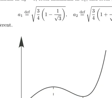
The graph of J, shown in Figure 1.1, is not the graph of a convex function. Its global minimum in a0= 0, local maximum in a1, and local minimum in a2,
a1def= " 3 4 # 1 −√13 $ , a2def= " 3 4 # 1 + √13 $ , are all different.
a1 a2
Figure 1.1. Graph of J(a).
To avoid a trivial solution, a strictly positive lower bound must be put on a. A unique minimizing solution is obtained for a ≥ a1where the gradient of J is zero.
For 0 < a < a2, the minimum will occur at the preset lower or upper bound on a.
3 Buckling of Columns
The next example illustrates the fact that even simple problems can be nondiffer-entiable with respect to the geometry. This is generic of all eigenvalue problems when the eigenvalue is not simple.
One of the early optimal design problems was formulated by J. L. Lagrange [1] in 1770 (cf. I. Todhunter and K. Pearson [1]) and later studied by the Danish mathematician and astronomer T. Clausen [1] in 1849. It consists in finding the best profile of a vertical column of fixed volume to prevent buckling.
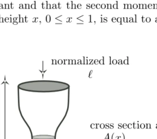
It turns out that this problem is in fact a hidden maximization of an eigenvalue. Many incorrect solutions had been published until 1992. This problem and other problems related to columns have been revisited in a series of papers by S. J. Cox [1], S. J. Cox and M. L. Overton [1], S. J. Cox [2], and S. J. Cox and C. M. McCarthy [1]. Since Lagrange many authors have proposed solutions, but a complete theoretical and numerical solution for the buckling of a column was given only in 1992 by S. J. Cox and M. L. Overton [1]. The difficulty was that the eigenvalue is not simple and hence not differentiable with respect to the geometry. Consider a normalized column of unit height and unit volume (see Figure 1.2). Denote by ℓ the magnitude of the normalized axial load and by u the resulting transverse displacement. Assume that the potential energy is the sum of the bending and elongation energies
! 1 0 EI|u
′′|2dx− ℓ! 1 0 |u
′|2dx,
where I is the second moment of area of the column’s cross section and E is its Young’s modulus. For sufficiently small load ℓ the minimum of this potential energy with respect to all admissible u is zero. Euler’s buckling load λ of the column is the largest ℓ for which this minimum is zero. This is equivalent to finding the following minimum: λdef= inf 0̸=u∈V %1 0 EI|u′′|2dx %1 0 |u′|2dx , (3.1) where V = H2
0(0, 1) corresponds to the clamped case, but other types of
bound-ary conditions can be contemplated. This is an eigenvalue problem with a special Rayleigh quotient.
Assume that E is constant and that the second moment of area I(x) of the column’s cross section at the height x, 0 ≤ x ≤ 1, is equal to a constant c times its
0 x 1
normalized load ℓ
cross section area A(x)
cross-sectional area A(x),
I(x) = c A(x) and ! 1
0 A(x) dx = 1.
Normalizing λ by cE and taking into account the engineering constraints ∃0 < A0< A1,∀x ∈ [0, 1], 0 < A0≤ A(x) ≤ A1,
we finally get
sup
A∈A
λ(A), λ(A)def= inf
0̸=u∈V %1 0 A|u′′|2dx %1 0 |u′|2dx , (3.2) Adef= & A∈ L2(0, 1) : A0≤ A ≤ A1 and ! 1 0 A(x) dx = 1 ' . (3.3)
4 Eigenvalue Problems
Let D be a bounded open Lipschitzian domain in RNand A ∈ L∞(D; L(RN, RN))
be a matrix function defined on D such that
∗A = A and αI≤ A ≤ βI (4.1)
for some coercivity and continuity constants 0 < α ≤ β and ∗A is the transpose of
A. Consider the minimization or the maximization of the first eigenvalue sup Ω∈A(D)λ A(Ω) inf Ω∈A(D)λ A(Ω) ( ( ( ( ( ( ( λA(Ω)def= inf 0̸=ϕ∈H1 0(Ω) % ΩA%∇ϕ · ∇ϕ dx Ω|ϕ|2dx , (4.2) where A(D) is a family of admissible open subsets of D (cf., for instance, sections 2, 7, and 9 of Chapter 8).
In the vectorial case, consider the following linear elasticity problem: find U ∈ H01(Ω)3such that ∀W ∈ H01(Ω)3, ! ΩCε(U )·· ε(W ) dx = ! ΩF· W dx (4.3)
for some distributed loading F ∈ L2(Ω)3and a constitutive law C which is a bilinear
symmetric transformation of
Sym3def= )τ∈ L(R3; R3):∗τ = τ*, σ·· τ def= + 1≤i,j≤3
σijτij
(L(R3; R3) is the space of all linear transformations of R3or 3 × 3-matrices) under
the following assumption. Assumption 4.1.
The constitutive law is a transformation C ∈ Sym3for which there exists a constant
For instance, for the Lam´e constants µ > 0 and λ ≥ 0, the special constitutive law Cτ = 2µ τ + λ tr τ I satisfies Assumption 4.1 with α = 2µ.
The associated bilinear form is aΩ(U, W )def=
!
ΩCε(U )·· ε(W ) dx,
where U is a vector function, D(U) is the Jacobian matrix of U, and ε(U )def= 1
2(D(U) + ∗D(U ))
is the strain tensor. The first eigenvalue is the minimum of the Rayleigh quotient λ(Ω) = inf & a Ω(U, U) % Ω|U|2dx : ∀U ∈ H 1 0(Ω)3, U ̸= 0 ' .
A typical problem is to find the sensitivity of the first eigenvalue with respect to the shape of the domain Ω. In 1907, J. Hadamard [1] used displacements along the normal to the boundary Γ of a C∞-domain to compute the derivative of the
first eigenvalue of the clamped plate. As in the case of the column, this problem is not differentiable with respect to the geometry when the eigenvalue is not simple.
5 Optimal Triangular Meshing
The shape calculus that will be developed in Chapters 9 and 10 for problems gov-erned by partial differential equations (the continuous model) will be readily ap-plicable to their discrete model as in the finite element discretization of elliptic boundary value problems. However, some care has to be exerted in the choice of the formula for the gradient, since the solution of a finite element discretization problem is usually less smooth than the solution of its continuous counterpart.
Most shape objective functionals will have two basic formulas for their shape gradient: a boundary expression and a volume expression. The boundary expression is always nicer and more compact but can be applied only when the solution of the underlying partial differential equation is smooth and in most cases smoother than the finite element solution. This leads to serious computational errors. The right formula to use is the less attractive volume expression that requires only the same smoothness as the finite element solution. Numerous computational experiments confirm that fact (cf., for instance, E. J. Haug and J. S. Arora [1] or E. J. Haug, K. K. Choi, and V. Komkov [1]). With the volume expression, the gradient of the objective function with respect to internal and boundary nodes can be readily obtained by plugging in the right velocity field.
A large class of linear elliptic boundary value problems can be expressed as the minimum of a quadratic function over some Hilbert space. For instance, let Ω be a bounded open domain in RN with a smooth boundary Γ. The solution u of
the boundary value problem
is the minimizing element in the Sobolev space H1
0(Ω) of the energy functional
E(v, Ω)def= ! Ω|∇v| 2 − 2f v dx, J(Ω)def= inf v∈H1 0(Ω) E(v, Ω) = E(u, Ω) =− ! Ω|∇u| 2dx.
The elements of this problem are a Hilbert space V , a continuous symmetrical co-ercive bilinear form on V , and a continuous linear form ℓ on V . With this notation
∃u ∈ V, E(u) = infv
∈VE(v), E(v) def
= a(v, v) − 2 ℓ(v) and u is the unique solution of the variational equation
∃u ∈ U, ∀v ∈ V, a(u, v) = ℓ(v).
In the finite element approximation of the solution u, a finite-dimensional subspace Vh of V is used for some small mesh parameter h. The solution of the
approximate problem is given by ∃uh∈ Vh, E(uh) = inf
vh∈Vh
E(vh), ⇒ ∃uh∈ Uh, ∀vh∈ Vh, a(uh, vh) = ℓ(vh).
It is easy to show that the error can be expressed as follows: a(u− uh, u− uh) = ∥u − uh∥2V = 2 [E(uh) − E(u)] .
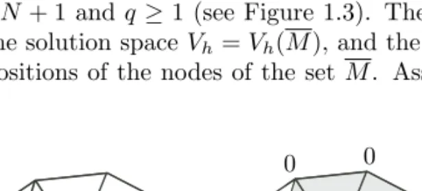
Assume that Ω is a polygonal domain in RN. In the finite element method, the
domain is partitioned into a set τhof small triangles by introducing nodes in ¯Ω
M def= {Mi∈ Ω : 1 ≤ i ≤ p}
∂M def= {Mi∈ ∂Ω : p + 1 ≤ i ≤ p + q}
and Mdef= M ∪ ∂M
for some integers p ≥ N + 1 and q ≥ 1 (see Figure 1.3). Therefore the triangular-ization τh= τh(M), the solution space Vh= Vh(M), and the solution uh= uh(M)
are functions of the positions of the nodes of the set M. Assuming that the total
Mi 1 0 0 0 0 0 0
number of nodes is fixed, consider the following optimal triangularization problem: inf
M
j(M ), j(M )def= E(uh(τh(M)), Ω) = inf vh∈Vh(M) E(vh, Ω), ∥u − uh∥2V = ! Ω|∇(u − uh)| 2dx = 2,E(u h, Ω(τh(M))) − E(u, Ω) -= 2 ,J(Ω(τh(M))) − J(Ω)-, J(Ω(τh(M)))def= inf vh∈Vh E(vh, Ω(τh(M))) = E(uh, Ω(τh(M))) = − ! Ω|∇uh| 2dx.
The objective is to compute the partial derivative of j(M) with respect to the ℓth component (Mi)ℓ of the node Mi:
∂j ∂(Mi)ℓ
(M).
This partial derivative can be computed by using the velocity method for the special velocity field (cf. M. C. Delfour, G. Payre, and J.-P. Zol´esio [3])
Viℓ(x) = bMi(x) ⃗eℓ,
where bMi ∈ Vh is the (piecewise P1) basis function associated with the node Mi:
bMi(Mj) = δij for all i, j. In that method each point X of the plane is moved
according to the solution of the vector differential equation dx
dt(t) = V (x(t)), x(0) = X.
This yields a transformation X .→ Tt(X)def= x(t; X) : R2→ R2 of the plane, and it
is natural to introduce the following notion of semiderivative: dJ(Ω; V )def= lim
t↘0
J(Tt(Ω)) − J(Ω)
t .
For t ≥ 0 small, the velocity field must be chosen in such a way that triangles are moved onto triangles and the point Miis moved in the direction ⃗eℓ:
Mi→ Mit= Mi+ t ⃗eℓ.
This is achieved by choosing the following velocity field: Viℓ(t, x) = bMit(x) ⃗eℓ,
where bMit is the piecewise P
1basis function associated with node M
it: bMit(Mj) =
δij for all i, j. This yields the family of transformations
Tt(x) = x + t bMi(x) ⃗eℓ
which moves the node Mi to Mi+ t ⃗eℓ and hence
∂j ∂(Mi)ℓ
Going back to our original example, introduce the shape functional J(Ω)def= inf v∈H10(Ω) E(Ω, v) =− ! Ω|∇u| 2dx, E(Ω, v) =! Ω|∇v| 2 − 2 f v dx. In Chapter 9, we shall show that we have the following boundary and volume ex-pressions for the derivative of J(Ω):
dJ(Ω; V ) =− ! Γ ( ( ( (∂u∂n ( ( ( ( 2 V · n dΓ, dJ(Ω; V ) = ! ΩA
′(0)∇u · ∇u − 2 [div V (0)f + ∇f · V (0)] u dx,
A′(0) = div V (0) I − ∗DV (0)− DV (0). For a P1-approximation
Vhdef=)v∈ C0(¯Ω) : v|K ∈ P1(K), ∀K ∈ τh*
and the trace of the normal derivative on Γ is not defined. Thus, it is necessary to use the volume expression. For the velocity field Viℓ
DViℓ= ⃗eℓ∗∇bMi, div DViℓ= ⃗eℓ· ∇bMi,
A′(0) = ⃗eℓ· ∇bMiI− ⃗eℓ∗∇bMi− ∇bMi∗⃗eℓ.
Since
∂j ∂(Mi)ℓ
(M) = dJ(Ω; Viℓ),
we finally obtain the formula for the derivative of the function j(M) with respect to node Mi in the direction ⃗eℓ:
∂j ∂(Mi)ℓ (M) =! Ω[⃗eℓ· ∇bMiI− ⃗eℓ ∗∇b Mi− ∇bMi ∗⃗e ℓ] ∇; uh· ∇uh − 2 [⃗eℓ· ∇bMif +∇f · ⃗eℓbMi] uhdx.
Since the support of bMi consists of the triangles having Mias a vertex, the gradient
with respect to the nodes can be constructed piece by piece by visiting each node.
6 Modeling Free Boundary Problems
The first step towards the solution of a shape optimization is the mathematical modeling of the problem. Physical phenomena are often modeled on relatively smooth or nice geometries. Adding an objective functional to the model will usually push the system towards rougher geometries or even microstructures. For instance, in the optimal design of plates the optimization of the profile of a plate led to highly oscillating profiles that looked like a comb with abrupt variations ranging from zero
to maximum thickness. The phenomenon began to be understood in 1975 with the paper of N. Olhoff [1] for circular plates with the introduction of the mechanical notion of stiffeners. The optimal plate was a virtual plate, a microstructure, that is a homogenized geometry. Another example is the Plateau problem of minimal surfaces that experimentally exhibits surfaces with singularities. In both cases, it is mathematically natural to replace the geometry by a characteristic function, a function that is equal to 1 on the set and 0 outside the set. Instead of optimizing over a restricted family of geometries, the problem is relaxed to the optimization over a set of measurable characteristic functions that contains a much larger family of geometries, including the ones with boundary singularities and/or an arbitrary number of holes.
6.1 Free Interface between Two Materials
Consider the optimal design problem studied by J. C´ea and K. Malanowski [1] in 1970, where the optimization variable is the distribution of two materials with different physical characteristics within a fixed domain D. It cannot a priori be assumed that the two regions are separated by a smooth interface and that each region is connected. This problem will be covered in more details in section 4 of Chapter 5.
Let D ⊂ RN be a bounded open domain with Lipschitzian boundary ∂D.
Assume for the moment that the domain D is partitioned into two subdomains Ω1
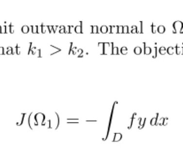
and Ω2 separated by a smooth interface ∂Ω1∩ ∂Ω2 as illustrated in Figure 1.4.
Domain Ω1(resp., Ω2) is made up of a material characterized by a constant k1> 0
(resp., k2> 0). Let y be the solution of the transmission problem
⎧ ⎨ ⎩
− k1△y = f in Ω1 and − k2△y = f in Ω2,
y = 0 on ∂D and k1∂n∂y 1 + k2
∂y
∂n2 = 0 on Ω1∩ Ω2,
(6.1) where n1 (resp., n2) is the unit outward normal to Ω1 (resp., Ω2) and f is a given
function in L2(D). Assume that k
1> k2. The objective is to maximize the
equiva-lent of the compliance
J(Ω1) = − ! D f y dx (6.2) Ω2 Ω1
over all domains Ω1 in D subject to the following constraint on the volume of
material k1 which occupies the part Ω1 of D:
m(Ω1) ≤ α, 0 < α < m(D) (6.3)
for some constant α.
If χ denotes the characteristic function of the domain Ω1,
χ(x) = 1 if x∈ Ω1and 0 if x /∈ Ω1,
the compliance J(χ) = J(Ω1) can be expressed as the infimum over the Sobolev
space H1
0(D) of an energy functional defined on the fixed set D:
J(χ) = min ϕ∈H01(D) E(χ, ϕ), (6.4) E(χ, ϕ)def= ! D (k1χ + k2(1 − χ)) |∇ϕ|2− 2 χfϕ dx. (6.5)
J(χ) can be minimized or maximized over some appropriate family of characteristic functions or with respect to their relaxation to functions between 0 and 1 that would correspond to microstructures. As in the eigenvalue problem, the objective function is an infimum, but here the infimum is over a space that does not depend on the function χ that specifies the geometric domain. This will be handled by the special techniques of Chapter 10 for the differentiation of the minimum of a functional.
6.2 Minimal Surfaces
The celebrated Plateau’s problem, named after the Belgian physicist and profes-sor J. A. F. Plateau [1] (1801–1883), who did experimental observations on the geometry of soap films around 1873, also provides a nice example where the geome-try is a variable. It consists in finding the surface of least area among those bounded by a given curve. One of the difficulties in studying the minimal surface problem is the description of such surfaces in the usual language of differential geometry. For instance, the set of possible singularities is not known.
Measure theoretic methods such as k-currents (k-dim surfaces) were used by E. R. Reifenberg [1, 2, 3, 4] around 1960, H. Federer and W. H. Fleming [1] in 1960 (normals and integral currents), F. J. Almgren, Jr. [1] in 1965 (varifolds), and H. Federer [5] in 1969.
In the early 1950s, E. De Giorgi [1, 2, 3] and R. Caccioppoli [1] considered a hypersurface in the N-dimensional Euclidean space RN as the boundary of a
set. In order to obtain a boundary measure, they restricted their attention to sets whose characteristic function is of bounded variation. Their key property is an associated natural notion of perimeter that extends the classical surface measure of the boundary of a smooth set to the larger family of Caccioppoli sets named after the celebrated Neapolitan mathematician Renato Caccioppoli.2
2In 1992 his tormented personality was remembered in a film directed by Mario Martone, The
Caccioppoli sets occur in many shape optimization problems (or free boundary problems), where a surface tension is present on the (free) boundary, such as in the free interface water/soil in a dam (C. Baiocchi, V. Comincioli, E. Magenes, and G. A. Pozzi [1]) in 1973 and in the free boundary of a water wave (M. Souli and J.-P. Zol´esio [1, 2, 3, 4, 5]) in 1988. More details will be given in Chapter 5.
7 Design of a Thermal Diffuser
Shape optimization problems are everywhere in engineering, physics, and medicine. We choose two illustrative examples that were proposed by the Canadian Space Program in the 1980s. The first one is the design of a thermal diffuser to condi-tion the thermal environment of electronic devices in communicacondi-tion satellites; the second one is the design of a thermal radiator that will be described in the next sec-tion. There are more and more design and control problems coming from medicine. For instance, the design of endoprotheses such as valves, stents, and coils in blood vessels or left ventricular assistance devices (cardiac pumps) in interventional car-diology helps to improve the health of patients and minimize the consequences and costs of therapeutical interventions by going to mini-invasive procedures.
7.1 Description of the Physical Problem
This problem arises in connection with the use of high-power solid-state devices (HPSSD) in communication satellites (cf. M. C. Delfour, G. Payre, and J.-P. Zol´esio [1]). An HPSSD dissipates a large amount of thermal power (typ. > 50 W) over a relatively small mounting surface (typ. 1.25 cm2). Yet, its junction temperature is required to be kept moderately low (typ. 110◦C). The thermal
resistance from the junction to the mounting surface is known for any particular HPSSD (typ. 1◦C/W), so that the mounting surface is required to be kept at
a lower temperature than the junction (typ. 60◦C). In a space application the
thermal power must ultimately be dissipated to the environment by the mechanism of radiation. However, to radiate large amounts of thermal power at moderately low temperatures, correspondingly large radiating areas are required. Thus we have the requirement to efficiently spread the high thermal power flux (TPF) at the HPSSD source (typ. 40 W/cm2) to a low TPF at the radiator (typ. 0.04 W/cm2) so that
the source temperature is maintained at an acceptably low level (typ. < 60◦C)
at the mounting surface. The efficient spreading task is best accomplished using heatpipes, but the snag in the scheme is that heatpipes can accept only a limited maximum TPF from a source (typ. max 4 W/cm2).
Hence we are led to the requirement for a thermal diffuser. This device is inserted between the HPSSD and the heatpipes and reduces the TPF at the source (typ. > 40 W/cm2) to a level acceptable to the heatpipes (typ. > 4 W/cm2). The
heatpipes then sufficiently spread the heat over large space radiators, reducing the TPF from a level at the diffuser (typ. 4 W/cm2) to that at the radiator (typ. 0.04
W/cm2). This scheme of heat spreading is depicted in Figure 1.5.
It is the design of the thermal diffuser which is the problem at hand. We may assume that the HPSSD presents a uniform thermal power flux to the diffuser