Preindustrial-to-present-day radiative forcing by tropospheric ozone from improved simulations with the GISS chemistry-climate GCM

HAL Id: hal-00295342

https://hal.archives-ouvertes.fr/hal-00295342

Submitted on 10 Oct 2003

HAL is a multi-disciplinary open access

archive for the deposit and dissemination of

sci-entific research documents, whether they are

pub-lished or not. The documents may come from

teaching and research institutions in France or

abroad, or from public or private research centers.

L’archive ouverte pluridisciplinaire HAL, est

destinée au dépôt et à la diffusion de documents

scientifiques de niveau recherche, publiés ou non,

émanant des établissements d’enseignement et de

recherche français ou étrangers, des laboratoires

publics ou privés.

tropospheric ozone from improved simulations with the

GISS chemistry-climate GCM

D. T. Shindell, G. Faluvegi, N. Bell

To cite this version:

D. T. Shindell, G. Faluvegi, N. Bell. Preindustrial-to-present-day radiative forcing by tropospheric

ozone from improved simulations with the GISS chemistry-climate GCM. Atmospheric Chemistry and

Physics, European Geosciences Union, 2003, 3 (5), pp.1675-1702. �hal-00295342�

www.atmos-chem-phys.org/acp/3/1675/

Chemistry

and Physics

Preindustrial-to-present-day radiative forcing by tropospheric ozone

from improved simulations with the GISS chemistry-climate GCM

NASA Goddard Institute for Space Studies, and Center for Climate Systems Research, Columbia University, New York, New York, USA

Received: 22 May 2003 – Published in Atmos. Chem. Phys. Discuss.: 28 July 2003 Revised: 2 October 2003 – Accepted: 6 October 2003 – Published: 10 October 2003

Abstract. Improved estimates of the radiative forcing from tropospheric ozone increases since the preindustrial have been calculated with the tropospheric chemistry model used at the Goddard Institute for Space Studies (GISS) within the GISS general circulation model (GCM). The chemistry in this model has been expanded to include simplified repre-sentations of peroxyacetylnitrates and non-methane hydro-carbons in addition to background NOx-HOx-Ox-CO-CH4

chemistry. The GCM has improved resolution and physics in the boundary layer, improved resolution near the tropopause, and now contains a full representation of stratospheric dy-namics. Simulations of present-day conditions show that this coupled chemistry-climate model is better able to reproduce observed tropospheric ozone, especially in the tropopause region, which is critical to climate forcing. Comparison with preindustrial simulations gives a global annual aver-age radiative forcing due to tropospheric ozone increases of 0.30 W/m2with standard assumptions for preindustrial emis-sions. Locally, the forcing reaches more than 0.8 W/m2 in parts of the northern subtropics during spring and summer, and is more than 0.6 W/m2 through nearly all the North-ern subtropics and mid-latitudes during summer. An alter-native preindustrial simulation with soil NOx emissions

re-duced by two-thirds and emissions of isoprene, paraffins and alkenes from vegetation increased by 50% gives a forcing of 0.33 W/m2. Given the large uncertainties in preindustrial ozone amounts, the true value may lie well outside this range.

1 Introduction

Changes in atmospheric chemistry since the industrial revo-lution have had a significant impact on climate and human health, but are difficult to quantify accurately due to their

Correspondence to: D. T. Shindell

(dshindell@giss.nasa.gov)

complexity (Intergovernmental Panel on Climate Change (hereafter IPCC), 2001). Increased anthropogenic emissions of ozone precursor gases such as nitrogen oxides (NOx)

pro-duce tropospheric ozone, a potent greenhouse gas, and also alter the oxidation capacity of the troposphere. The latter change affects the lifetime of many trace gases, including methane, another powerful greenhouse gas. Tropospheric ozone changes have a spatial pattern that is extremely inho-mogeneous, leading to similar inhomogenaity in its radiative forcing. We therefore feel it is useful to explore these chemi-cal changes in a model in which they can be directly coupled to the concurrent climate changes during the past and those projected for the future.

The magnitude of the radiative forcing due to tropospheric ozone increases is relatively uncertain. This uncertainty arises from the paucity of observations during the prein-dustrial period, and the poor quality of those that do ex-ist. Estimates are therefore based on model simulations, though these are subject to large uncertainties in the emis-sions of ozone precursors in both modern and especially in preindustrial times, as well as in chemical and physi-cal processes. Though the IPCC presents estimates of the forcing from tropospheric ozone since the preindustrial of

+0.35±0.15 W/m2, several recent studies have indicated that the value may actually be significantly larger. These studies are based upon preindustrial emissions of precursors adjusted within their uncertainties to give a better match to the pur-ported 19th century observations of surface ozone (Mickley et al., 2001), or estimates constrained by 20th century ob-servations prior to the late 1970s onset of large amounts of stratospheric ozone depletion by chlorofluorocarbons (Shin-dell and Faluvegi, 2002). Both studies find that forcings of around 0.7 W/m2are reasonable.

Radiative forcing from tropospheric ozone is especially large (per unit ozone change) near the tropopause (Hansen et al., 1997; Hauglustaine and Brasseur, 2001). Estimates of ozone change in this region are therefore especially

important for evaluating ozone’s forcing. Ozone in this re-gion is extremely sensitive to stratosphere-troposphere ex-change and to production of NOx by lightning (Grewe et

al., 2001). Both these factors are only weakly constrained by present-day observations, and are largely unconstrained for the preindustrial era. It is therefore a priority that the chemistry-climate models used to estimate tropospheric ozone’s radiative forcing provide accurate simulations in this region.

We have previously developed and evaluated a simplified tropospheric chemistry package within the GISS GCM and used that model to explore the preindustrial to present-day radiative forcing from tropospheric ozone (Shindell et al., 2001). That model has also been applied to studies of the relative importance of individual emission changes and cli-mate responses since the preindustrial (Grenfell et al., 2001) amd for the future (Grenfell et al., 2003), to an investiga-tion of the origin and variability of upper tropospheric nitro-gen oxides and ozone (Grewe et al., 2001), and to a study of dynamical-chemical coupling across the tropopause (Grewe et al., 2002). Comparison with observations for that model showed that it was able to simulate tropospheric ozone and related species reasonably well. However, with only 9 ver-tical layers, that model had very coarse resolution in the vicinity of the tropopause and a poor representation of the stratosphere, so that its primary deficiency was in simulat-ing stratosphetroposphere exchange and tropopause re-gion ozone accurately. We present here a new version of the GISS coupled chemistry-climate model with greater ver-tical resolution and a full representation of the stratosphere (though without stratospheric chemistry). Given the result-ing large increase in the computational expense of the climate model portion of the simulation, it was relatively inexpen-sive to add to the chemistry. We have therefore expanded the original simple HOx-NOx-Ox-CO-CH4chemistry to include

isoprene and the peroxyacetylnitrate (PAN), alkene, alkyl ni-trate, paraffin and aldehyde families, thus providing a more realistic representation of tropospheric chemistry. This new model has been used to simulate present-day conditions, and has been extensively compared with observations. We have then performed preindustrial simulations, and investigated the resulting radiative forcing.

2 Model description 2.1 Chemistry

The model includes the basic HOx-NOx-Ox-CO-CH4

chemistry (HOx=OH+HO2; NOx=NO+NO2+NO3+HONO;

Ox=O+O(1D)+O3) described in Shindell et al. (2001), as

well as the additional molecules and chemical reactions shown in Tables 1 and 2. We make use of the “chemical family” approach, whereby reactions between family mem-bers are assumed to be rapid enough to maintain steady-state

(at night, however, NOx changes are explicitly calculated).

This allows a larger chemical time step and transport of the entire family as a single tracer. We also use “lumped fam-ilies” for hydrocarbons and PANs, which is necessary for the model to run sufficiently rapidly to be useful for climate studies. Chemical reactions involving these surrogates are based on the similarity between the molecular bond struc-tures within each family using the reduced chemical mecha-nism of Houweling et al. (1998). This mechamecha-nism is based on the Carbon Bond Mechanism-4 (CBM-4) (Gery et al., 1989), modified to better represent the globally important range of conditions. The CBM-4 scheme has been validated extensively against smog chamber experiments and more de-tailed chemical schemes (Gery et al., 1988; Derwent, 1990; Paulson and Seinfeld, 1992; Tonnesen and Jeffries, 1994). This scheme was modified for use in global models by re-moving aromatic compounds and adding in reactions im-portant in background conditions, including organic nitrate and organic peroxide reactions, and extending the methane oxidation chemistry. The revised scheme was then read-justed based on the more extensive Regional Atmospheric Chemistry Model (RACM) (Stockwell et al., 1997), and the modified scheme includes several surrogate species designed to compensate for biases relative to the RACM mechanism (XO2, XO2N, RXPAR and ROR; see Table 1 for detailed

de-scriptions). The modified scheme was shown to agree well with the detailed RACM reference mechanism over a wide range of chemical conditions including relatively pristine en-vironments (Houweling et al., 1998). Standard gas phase chemical reaction rates have been updated to recent values (Sander et al., 2000).

The chemical family approach of grouping radical species together, along with combining hydrocarbons with similar characteristics into lumped families, permits calculations re-quiring the transport of only sixteen species in the GCM (Ta-ble 1). After combining the short-lived radicals into equili-brated families, we find that nearly all the species have long enough lifetimes that we can use an extremely simple ex-plicit scheme to calculate chemical changes. The exceptions are HOx, CH3O2, C2O3, aldehydes and the surrogates XO2,

XO2N, RXPAR and ROR, whose very short lifetimes keep

them in equilibrium at all times. Calculations are performed using a chemical time step of 1 h.

The chemical scheme includes 77 reactions, 25 of which have been added to the previous scheme to account for reac-tions of PANs and NMHCs (Table 2). The chemistry includes changes in ozone from partitioning within the NOxfamily

to avoid spurious ozone sources or sinks associated with the separation of the Oxand NOxfamilies. As with the simpler

scheme, heterogeneous hydrolysis of N2O5into HNO3takes

place on sulfate aerosols, using the reaction rate coefficients given by Dentener and Crutzen (1993). Sulfate surface ar-eas are taken from an online calculation performed with the 9-layer version of the GISS GCM (Koch et al., 1999), as-suming a monodispersed size distribution. Photolysis rates

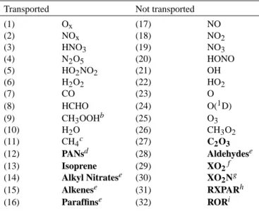
Table 1. Gases included in the model

Transported Not transported

(1) Ox (17) NO (2) NOx (18) NO2 (3) HNO3 (19) NO3 (4) N₂O₅ (20) HONO (5) HO2NO2 (21) OH (6) H₂O₂ (22) HO₂ (7) CO (23) O (8) HCHO (24) O(1D) (9) CH3OOHb (25) O3 (10) H2O (26) CH3O2 (11) CH4c (27) C2O3 (12) PANsd (28) Aldehydese (13) Isoprene (29) XO₂f (14) Alkyl Nitratese (30) XO2Ng (15) Alkenese (31) RXPARh (16) Paraffinse (32) RORi

a_{Additional gases in the more comprehensive chemistry scheme are in bold face type.}

b_{Methyl hydroperoxide also includes a small contribution from higher organic peroxides.}

c_{Transport of methane is optional.}

d_{PANs are peroxyacetylnitrate and higher PANs.}

e_{Alkyl Nitrates, Alkenes, Paraffins, and Aldehydes are lumped families. Alkenes include propene, >C3 alkenes, and >C2 alkynes,}

paraf-fins include ethane, propane, butane, pentane, >C5 alkanes and ketones, while aldehydes include acetaldehyde and higher aldehydes (not formaldehyde).

f _XO

2is a surrogate species to represent primarily hydrocarbon oxidation byproducts that subsequently convert NO to NO2, and also leads

to a small amount of organic peroxide formation. g_XO

2N is a surrogate species to represent hydrocarbon oxidation byproducts that subsequently convert NO to alkyl nitrates, and also leads

to a small amount of organic peroxide formation.

h_{RXPAR is a paraffin budget corrector to correct a bias in the oxidation of alkenes related to an overly short chain length for the lumped}

alkenes.

i_{ROR are radical byproducts of paraffin oxidation.}

are calculated every two hours using the Fast-J scheme (Wild et al., 2000), and interact with the GCM’s aerosol and cloud fields. Phase transformations of soluble species are calcu-lated based on the GCM’s internal cloud scheme. We in-clude transport within convective plumes, scavenging within and below updrafts, rainout within both convective and large-scale clouds, washout below precipitating regions, evapora-tion of falling precipitaevapora-tion, and both detrainment and evapo-ration from convective plumes (Koch et al., 1999; Shindell et al., 2001). Dry deposition is based on a resistance-in-series calculation and prescribed (i.e. uncoupled) vegetation as described in Shindell et al. (2001). Chemical calcula-tions are performed only in the troposphere in this version of the model (below 150 hPa), while stratospheric values of ozone, nitrogen oxides, and methane are prescribed accord-ing to satellite observations with seasonally varyaccord-ing abun-dances as in the standard GISS model (Hansen et al., 1996). This implicitly includes stratospheric loss of methane, while other gases with stratospheric sinks are relaxed towards zero based on their chemical lifetime.

The model also includes a full representation of the global methane cycle, including the chemical oxidation chain and detailed emissions and sinks. Though not crucial for the sim-ulations described here, calculation of methane as an active chemical constituent will allow for future investigations of interactions between climate change and methane emissions and oxidation. Note that water vapor is also an active chemi-cal tracer in this model, in contrast to most chemichemi-cal models which lack a detailed hydrological cycle, and can thus re-spond to changes in climate via surface temperatures and to altered circulation patterns.

2.2 Sources and sinks

Emissions of NOxand CO are largely unchanged from our

previous model, based largely on the Global Emissions In-ventory Activity (GEIA) data sets (Benkovitz et al., 1996; Olivier et al., 1996) and on Wang et al. (1998a). Total emissions of CO are 987.7 Tg/yr (490.1 from biomass burn-ing and 497.6 from industrial activities). Prescribed emis-sions of NOxwere 20.9 Tg/yr N from fossil fuels, 5.8 from

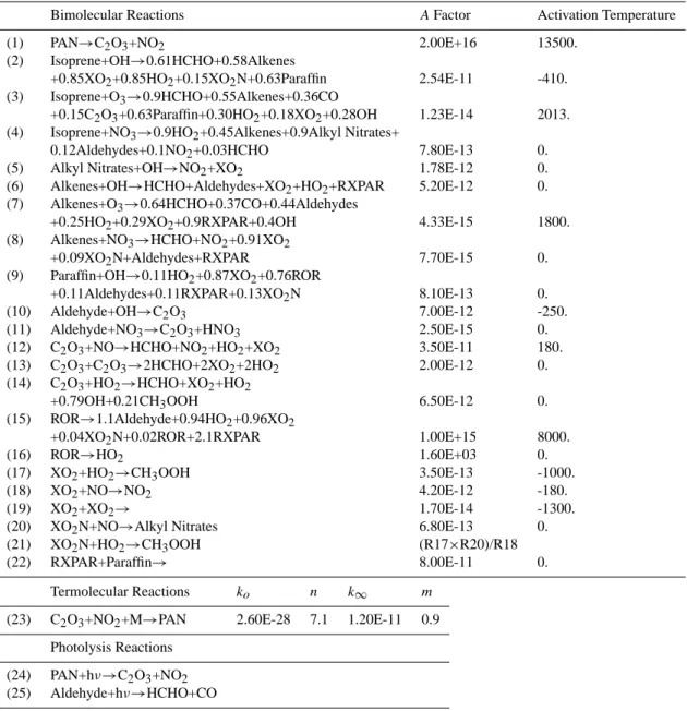
Table 2. Additional reactions included in the modela

Bimolecular Reactions AFactor Activation Temperature

(1) PAN→C2O3+NO2 2.00E+16 13500.

(2) Isoprene+OH→0.61HCHO+0.58Alkenes

+0.85XO2+0.85HO2+0.15XO2N+0.63Paraffin 2.54E-11 -410.

(3) Isoprene+O₃→0.9HCHO+0.55Alkenes+0.36CO

+0.15C2O3+0.63Paraffin+0.30HO2+0.18XO2+0.28OH 1.23E-14 2013.

(4) Isoprene+NO₃→0.9HO₂+0.45Alkenes+0.9Alkyl Nitrates+

0.12Aldehydes+0.1NO2+0.03HCHO 7.80E-13 0.

(5) Alkyl Nitrates+OH→NO2+XO2 1.78E-12 0.

(6) Alkenes+OH→HCHO+Aldehydes+XO2+HO2+RXPAR 5.20E-12 0.

(7) Alkenes+O3→0.64HCHO+0.37CO+0.44Aldehydes

+0.25HO2+0.29XO2+0.9RXPAR+0.4OH 4.33E-15 1800.

(8) Alkenes+NO3→HCHO+NO2+0.91XO2

+0.09XO₂N+Aldehydes+RXPAR 7.70E-15 0.

(9) Paraffin+OH→0.11HO2+0.87XO2+0.76ROR

+0.11Aldehydes+0.11RXPAR+0.13XO₂N 8.10E-13 0.

(10) Aldehyde+OH→C2O3 7.00E-12 -250.

(11) Aldehyde+NO3→C2O3+HNO3 2.50E-15 0.

(12) C2O3+NO→HCHO+NO2+HO2+XO2 3.50E-11 180.

(13) C2O3+C2O3→2HCHO+2XO2+2HO2 2.00E-12 0.

(14) C₂O₃+HO₂→HCHO+XO₂+HO₂

+0.79OH+0.21CH3OOH 6.50E-12 0.

(15) ROR→1.1Aldehyde+0.94HO₂+0.96XO₂

+0.04XO2N+0.02ROR+2.1RXPAR 1.00E+15 8000.

(16) ROR→HO2 1.60E+03 0.

(17) XO2+HO2→CH3OOH 3.50E-13 -1000.

(18) XO2+NO→NO2 4.20E-12 -180.

(19) XO2+XO2→ 1.70E-14 -1300.

(20) XO2N+NO→Alkyl Nitrates 6.80E-13 0.

(21) XO₂N+HO₂→CH₃OOH (R17×R20)/R18

(22) RXPAR+Paraffin→ 8.00E-11 0.

Termolecular Reactions ko n k∞ m

(23) C₂O₃+NO₂+M→PAN 2.60E-28 7.1 1.20E-11 0.9

Photolysis Reactions

(24) PAN+hν→C2O3+NO2

(25) Aldehyde+hν→HCHO+CO

a _{Reaction rates for bimolecular reactions are given by A exp ((−E/R)(1/T ), where A is the Arrhenius A factor, E/R is the activation}

temperature of the reaction, and T is the temperature. For termolecular reactions, rates are calculated as a function of the high- and

low-pressure reactions rates, given by k∞(T /300)-m and ko(T /300)-n, respectively, where T is temperature. In all the above reactions, M is

any body that can serve to carry away excess energy. For reaction 21, the rate is calculated based on the reaction rates of other reactions, as indicated. All rate coefficients taken from Houweling et al (1998).

b_{Read 2.00E+16 as 2.00×10}+16_.

soils, 5.8 from biomass burning, and 0.6 from aircraft (for comparison, internally generated lightning emissions were 6.5 Tg/yr). We have added emissions of isoprene based on Wang et al. (1998a), and alkenes and paraffins also based on GEIA. Global annual average emissions of isoprene were scaled to 200 Tg/yr from vegetation, as in recent model inter-comparisons (IPCC, 2001). Global annual average emissions of alkenes are 32.9 Tg/yr, made up of 16.0 Tg/yr from vege-tation, 11.6 Tg/yr from industry, and 5.3 Tg/yr from biomass

burning. The largest single contributor is propene, which makes up nearly half the emissions for this family, with other alkenes and alkynes also contributing. Global annual average emissions of paraffins are 87.0 Tg/yr, made up of 14.0 Tg/yr from vegetation, 68.8 Tg/yr from industry, and 4.2 Tg/yr from biomass burning. For the industrial component, bu-tane, pentane and higher alkanes are the largest sources, with smaller contributions from ethane and propane. The biomass burning component is dominated by ethane emissions. For

both the alkene and paraffin families, the spatial and temporal distribution of isoprene emissions was used for vegetation, and that of carbon monoxide for biomass burning, for lack of further information, with the overall source value scaled to the emissions given above. Distributions of industrial emis-sions of alkenes and paraffins are from GEIA.

Methane emissions were based upon the data sets of Fung et al. (1991) (available at http://www.giss.nasa.gov/data/ ch4fung). These fields were scaled to values within recent estimates of individual source strengths and their uncertain-ties (World Meteorological Organization (hereafter WMO), 1999), but maintaining the spatial distributions of the orig-inal data sets. The only exception was wetland emissions, which were shifted in latitude towards the tropics (x 1/3 pole-ward of 30◦in both hemispheres, x 10/4 from 30◦S–30◦N) to match more recent estimates of their meridional distribu-tion (WMO, 1995), and increased in magnitude to be more in line with recent estimates (Hein et al., 1997; Walter et al., 2001). Total emissions are 464.0 Tg/yr, made up of emis-sions from the following individual sources (in Tg/yr): an-imals (enteric fermentation in ruminants plus animal waste) 83.9, coal mining 20.1, pipeline leakage of natural gas 24.8, venting of natural gas at wells 17.0, landfills (including mu-nicipal solid waste) 27.5, termites 20.0, coal burning 16.0, ocean (including 3.0 from hydrates) 13.0, fresh water 5.0, miscellaneous ground sources (volcanoes and hydrothermal vents) 7.0, biomass burning 30.0, rice cultivation 30.0, wet-lands and tundra 209.7. Loss of methane via absorption into soils is also included, with a value of −39.9 Tg/yr (Fung et al., 1991; WMO, 1994). Biomass burning, rice cultivation and wetlands/tundra include seasonal emission cycles.

As in the older model, the GISS convection scheme is used to derive both the total lightning and the cloud-to-ground lightning frequencies interactively in each grid box and at each time step (Price et al., 1997). Then the generation of NOx from lightning is used to derive the NOx produced,

including a C-shaped vertical distribution (Pickering et al., 1998).

2.3 Climate model

The climate model used here is a version of the GISS model II’ (two-prime) enhanced over that used previously with updated planetary boundary layer and convection schemes. Briefly, the GCM’s boundary layer employs a finite modified Ekman layer with parameterizations for drag and mixing co-efficients based on similarity theory, convection includes en-training and nonenen-training plumes, mass fluxes proportional to convective instability, explicit downdrafts, and a cloud liq-uid water scheme, based on microphysical sources and sinks of cloud water, which carries both water and ice (Del Ge-nio et al., 1996). Simulations of the response to the erup-tion of Mt. Pinatubo with a similar version of the GCM (Hansen et al., 1996) show that the tropospheric water va-por response is comparable to observations. This provides

1000 100 10 9 layer GCM 23 layer GCM 1 hP a

Fig. 1. Vertical layering in the older 9-layer model (layer centers at 959, 894, 786, 634, 468, 321, 201, 103, and 26.5 hPa) and in the new 23-layer model (layer centers at 972, 945, 907, 852, 765, 640, 498, 370, 280, 219, 171, 134, 102, 71.2, 43.9, 24.7, 13.9, 7.32, 3.05, 0.960, 0.303, 0.088, and 0.017 hPa). The four highest layers of the 23-layer model are not shown.

some evidence that the response of the hydrological cycle to climate forcing in the GCM is realistic. The land surface pa-rameterization calculates transpiration, infiltration, soil water flow and runoff, all of which impact both water vapor and la-tent heat release to the atmosphere. Chemical tracers, along with heat and moisture, are advected using a quadratic up-stream scheme (Prather, 1986). Momentum advection uses a fourth-order scheme. The model’s interhemispheric ex-change time is 1.45 years (defined here as the difference in annual average mean methane mass between the hemispheres dived by the net annual average cross-equatorial mass flux), within 15–25% of values deduced from observations. Within the GISS chemistry modeling group we have focused on improving those aspects of the circulation that we believed would be most crucial for correctly simulating stratosphere-troposphere exchange. The gravity-wave drag scheme in this model version has been tested extensively and is now able to reproduce observed wind and temperature climatologies much better than in previous versions. This has led to notably improved transport of ozone down from the stratosphere, for example, which was heavily biased towards high latitudes and had an incorrect seasonal cycle in other model versions. All simulations with the new chemistry have been per-formed using a version with 4×5◦horizontal resolution and 23 vertical layers. Compared with the older model, the ver-tical resolution has been significantly improved in both the

boundary layer and near the tropopause, both regions cru-cial to ozone simulations, in addition to adding layers in the stratosphere (Fig. 1). The bottom 11 layers of this model are terrain-following levels, while the top 12 are constant pres-sure surfaces. The model time-step is one hour for both the chemistry and physics. Ozone calculated by the chemical model is coupled to the GCM’s radiation calculation, so that chemical changes are able to affect meteorology. Monthly mean sea-surface temperatures and sea ice cover are pre-scribed to 1990–1999 average values (Rayner et al., 2003) in these simulations for computational savings. Therefore the climate is not fully responsive to the chemistry. The importance of such coupling will be investigated in future simulations. All results presented here are averages over the last five years of seven year simulations. The model reaches equilibrium within the first year (methane values are pre-scribed according to observations, and other gases have life-times of about a month or less), and the interannual variabil-ity is relatively small compared to features of interest, so that five years gives us adequate statistics for mean values. The model has been run for present-day (1990) and for preindus-trial (∼1850) conditions. Additionally, a run with the older chemistry package lacking PANs and hydrocarbons higher than methane has been performed with the 23-layer GCM. This helps isolate the influence of the increased vertical res-olution from the effect of the more sophisticated chemistry.

The more comprehensive chemistry scheme adds only about 24% to the running time of the GCM, plus an addi-tional ∼15% for the transport of the chemical tracers, for a total increase of only ∼40%. It is therefore computationally rapid enough that the GCM can be run with online chem-istry for long-term climate simulations or for multiple runs to examine the sensitivity of the results to various changes. Though the fractional time used for chemistry is less for the more complex chemistry in the 23-layer model than for the simplified chemistry in the 9-layer model (∼40% versus

∼55%), this is only because the physics takes much longer in the 23-layer version, where the calculations are both more sophisticated and done on more vertical levels. The absolute time taken by the more complex chemistry is roughly a fac-tor of 3 greater than for the simplified chemistry, both due to the increase in the number of reactions and tracers and to the increase of nearly a factor of two in the number of vertical levels within the troposphere.

3 Evaluation of present-day simulation 3.1 Ozone

We have compared modeled annual cycles of ozone with the ozonesonde climatology of Logan (1999). Comparisons at stations representative of a wide range of latitudes are shown in Fig. 2. Results from the earlier 9-layer model with sim-plified chemistry are also shown (for these comparisons, we

have interpolated between model levels to the exact pressure levels of the sonde data, leading to slight differences as com-pared with the results shown for the older model in Shindell et al., 2001). The new model clearly does a better job at matching the observations than the older model at the lev-els nearest the tropopause (125 and 200 hPa). This holds for both the tropics, where the ozone is primarily of tropospheric origin, and for middle and high latitudes, where for at least part of the year the air is primarily of stratospheric origin. At 200 hPa, a positive bias in the tropics in the 9-layer model has been eliminated. Comparison of the results from the 23-layer simulations using simplified chemistry against those with the more advanced scheme show that the improvement in this region results primarily from an improved representation of tropical upwelling rather than from chemistry. The model has difficulty reproducing the spring maximum in ozone at 200 hPa at Northern middle and high latitudes, though it does this fairly well in the Southern Hemisphere. This maximum is stratospheric air, and thus may indicate biases in the strato-spheric ozone climatology. In fact, a minor flaw in the pre-scription of the climatology was discovered after completing the analysis of these simulations, which will be corrected in future work, and appears to correct the springtime values. It should also be noted that the vertical gradient of ozone is ex-tremely large at these altitudes, so that small differences in height can lead to ozone changes of hundreds of ppbv (this is true at 125 hPa as well). It may be that a near-perfect match with sondes can therefore only be obtained with ex-tremely high vertical resolution in this area. For those lo-cations and seasons dominated by tropospheric air (i.e. with ozone values less than about 150 ppbv, such as Hohenpeis-senberg during September and October and Lauder during January to April), the model does an excellent job of re-producing observed values. Results are fairly similar in the middle troposphere between the old and new models, though the positive bias at high latitudes is somewhat worse in the new version. Fortunately, these locations are less important for radiative forcing. Near the surface most locations show small improvements, while the comparison with Hohenpeis-senberg measurements is greatly improved. We attribute this largely to improvements in the boundary layer scheme of the GCM, including the higher vertical resolution there which allow more realistic dry deposition. Similar improvements in near-surface ozone values were seen at Pretoria and Sap-poro (not shown). Note that the sonde values at 950 hPa are interpolated from the reported observations at 1000 and 900 hPa where available, and are based upon the 900 hPa val-ues for the higher elevation sites where the 1000 hPa level is not available.

We compare the ability of the two model versions to repro-duce the observations over all the sites recommended for test-ing models by Logan(1999) in Table 3. As noted, the quality of the new model’s ozone simulation has improved markedly in the vicinity of the tropopause and near the surface. Biases in the vicinity of the tropopause are now very small. Though

1 2 3 4 5 6 7 8 9 10 11 12 200 400 600 800 1000 1200 1400 1600 1800 Resolute (75N) 125 hPa Ozone (ppbv) 1 2 3 4 5 6 7 8 9 10 11 12 100 250 400 550 700 850 1000 1150 Hohenpeissenberg (48N) 125 hPa Ozone (ppbv) 1 2 3 4 5 6 7 8 9 10 11 12 0 50 100 150 200 250 300 350 Hilo (20N) 125 hPa Ozone (ppbv) 1 2 3 4 5 6 7 8 9 10 11 12 0 100 200 300 400 500 600 700 800 900 200 hPa Ozone (ppbv) 1 2 3 4 5 6 7 8 9 10 11 12 0 100 200 300 400 500 600 200 hPa Ozone (ppbv) 1 2 3 4 5 6 7 8 9 10 11 12 0 25 50 75 100 125 150 200 hPa Ozone (ppbv) 1 2 3 4 5 6 7 8 9 10 11 12 0 100 200 300 400 300 hPa Ozone (ppbv) 1 2 3 4 5 6 7 8 9 10 11 12 0 50 100 150 200 300 hPa Ozone (ppbv) 1 2 3 4 5 6 7 8 9 10 11 12 0 25 50 75 100 125 150 300 hPa Ozone (ppbv) 1 2 3 4 5 6 7 8 9 10 11 12 0 25 50 75 100 125 150 500 hPa Ozone (ppbv) 1 2 3 4 5 6 7 8 9 10 11 12 0 25 50 75 100 125 150 500 hPa Ozone (ppbv) 1 2 3 4 5 6 7 8 9 10 11 12 0 25 50 75 100 125 150 500 hPa Ozone (ppbv) 1 2 3 4 5 6 7 8 9 10 11 12 0 25 50 75 100 950 hPa Month Ozone (ppbv) 1 2 3 4 5 6 7 8 9 10 11 12 0 25 50 75 100 950 hPa Month Ozone (ppbv) 1 2 3 4 5 6 7 8 9 10 11 12 0 25 50 75 100 950 hPa Month Ozone (ppbv)

Fig. 2. Comparison of observed and simulated annual cycles of ozone at the indicated pressure levels and locations. Solid and dotted lines indicate ozonesonde measured mean values and standard deviations, respectively. Solid circles show mean values from the new model while open triangles show values from the older model. All values are mixing ratios in ppbv, and model values have been interpolated to the given sonde pressure levels.

1 2 3 4 5 6 7 8 9 10 11 12 0 25 50 75 100 125 150 175 200

Natal (6S) 125 hPa

Lauder (45S) 125 hPa

Syowa (69S) 125 hPa

200 hPa

200 hPa

200 hPa

300 hPa

300 hPa

300 hPa

500 hPa

500 hPa

500 hPa

950 hPa

950 hPa

950 hPa

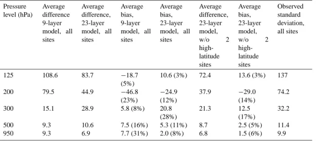
Table 3. Ozone differences (ppbv) between models and sondes Pressure level (hPa) Average difference 9-layer model, all sites Average difference, 23-layer model, all sites Average bias, 9-layer model, all sites Average bias, 23-layer model, all sites Average difference, 23-layer model, w/o 2 high-latitude sites Average bias, 23-layer model, w/o 2 high-latitude sites Observed standard deviation, all sites 125 108.6 83.7 −18.7 (5%) 10.6 (3%) 72.4 13.6 (3%) 137 200 79.5 44.9 −46.8 (23%) −24.9 (12%) 37.9 −29.0 (14%) 74.2 300 15.1 28.9 5.8 (8%) 20.8 (28%) 21.3 12.5 (17%) 32.2 500 9.3 10.6 7.5 (16%) 5.3 (11%) 8.7 2.5 (5%) 11.4 950 9.3 6.9 7.7 (31%) 2.0 (8%) 6.8 1.5 (6%) 9.9

Comparisons are between the 23-layer model and the 16 recommended sites of Logan (1999), having excluded the two sites with four months or less data. Average differences are from the month-by-month absolute value differences between the model and the sondes. Average biases are with no absolute value included. Values in parentheses are percent bias with respect to observed values at these levels. The sites are: Resolute, Edmonton, Hohenpeissenberg, Sapporo, Boulder, Wallops Island, Tateno, Kagoshima, Naha, Hilo, Natal, Samoa, Pretoria, Aspendale, Lauder, and Syowa.

the 125 hPa level is often in the stratosphere, and thus merely reflects the climatology, improvements in the tropics, where this level is in the troposphere, have reduced the bias there from 5% to 3% comparing the new model to the older ver-sion. At 200 hPa, the bias has been greatly reduced, from 23% to 12%. The average difference, for which positive and negative errors do not cancel out, has also dropped in this model, by 44% at 200 hPa. A similar level of improvement has been obtained at low levels, where biases have dropped to 11% and 8% at 500 and 950 hPa, respectively, from 16% and 31% in the older model. Similar improvements are ap-parent when examining the average absolute differences. In the middle troposphere, however, the average absolute differ-ence between the model and the observations has increased. Evaluation of the average bias reveals that this results largely from a consistent positive bias in this region, much of which comes from the two high-latitude sites (Table 3). This likely results from deficiencies in the GCM’s downward transport of stratospheric air at high latitudes, which also seems to af-fect the 500 hPa level at high latitudes. The positive bias at 300 hPa may also be related to the lightning NOxproduction,

which may be on the high side though it is well within current uncertainty (see below, and note that reduced lightning NOx

would worsen the negative bias at 200 hPa). Except for the 300 hPa level, however, the systematic bias averaged over all 16 sites is roughly 10% or less. The average absolute differ-ence between the model and the measurements is well within the observed standard deviation at all levels.

The model does a fairly good job of reproducing both the magnitude and seasonality of tropospheric ozone based on

the comparisons shown in Fig. 2, and is certainly improved over the previous simulations. While comparison between the 23-layer runs with simplified and advanced chemistry shows few obvious areas of improvement in the ozone fields, we nevertheless believe that incorporation of the advanced chemistry allows better simulation of tropospheric ozone in remote regions (where little validation data is available) and of ozone changes as a function of time, as well as doing a better job with other trace gases.

Surface ozone is shown in Fig. 3. Observations are well reproduced over most regions in this model. Beginning with remote regions, the model’s surface level ozone over the re-mote North Atlantic during January is slightly greater than observations, 35–45 ppbv as compared with measurements showing values of 30–40 ppbv (Parrish et al., 1998). The observational data however include only 4 years of measure-ments from Sable Island (44◦N, 60◦W) and a single year from the Azores (39◦N, 28◦W), so should be treated with some caution. At Izana (28◦N, 16◦W), slightly farther south over the Atlantic, the model underpredicts January ozone by 8.5 ppbv, and July ozone by 2.0 ppbv, while the annual av-erage model bias there is −7.0 ppbv. While the values are sometimes higher and sometimes lower than observations, overall the model seems to do a reasonable job over the re-mote Atlantic, though the model’s maximum may be too far north in January. The addition of PANs has increased the amount of ozone in remote regions of the Northern Hemi-sphere, causing an increase relative to the older model. In remote regions of the Southern Hemisphere, the model does an excellent job of reproducing the observed values. The

Fig. 3. Modeled ozone values (ppbv) in the lowest model layer for the present day. (top) January near-surface values, and (bottom) July values.

model finds July values of 25–35 ppbv at Syowa station, a location where most models underpredict ozone (Shindell et al., 2001). Over the Southern Hemisphere continents, surface ozone has decreased significantly compared with the previ-ous model version. For example, surface ozone over South America has dropped from 30–45 ppbv in the previous ver-sion to only 5–20 ppbv in the current model. The very low values seen in the new model during summer, 5–15 ppbv over the Amazon basin and 10–20 over the Brazilian savannah, are in agreement with measurements taken during the ABLE-2A summer campaign which showed near-surface ozone values of about 8–16 ppbv over the Amazon and slightly larger val-ues over the savannah (Kirchoff, 1988; Emmons et al., 2000). We attribute this change to the inclusion of non-methane hy-drocarbons, especially isoprene, which in regions with

rela-tively low abundances of NOxlead to ozone destruction.

Val-ues over the Southern Hemisphere oceans are quite similar in the two models, supporting a terrestrial influence.

A detailed comparison between land-based, primarily ru-ral surface ozone observations and the simulations has been made using the climatology of Logan (1999), based on data from 40 locations (Sanhueza et al., 1985; Cros et al., 1988; Kirchhoff and Rasmussen, 1990; Oltmans and Levy, 1994; Sunwoo and Carmichael, 1994). Results from a sample of sites are presented in Fig. 4. Clearly the model’s very low values over South America are in fact in good agree-ment with observations at Venezuela and Cuiaba. Sur-face ozone in the tropics is generally well-simulated, with both the large seasonal cycles at Bermuda and Japan Island and the smaller seasonality at Samoa, Barbados and Natal

1 2 3 4 5 6 7 8 9 10 11 12 0 10 20 30 40 50 60 70 80 23 layer model Observations 9 layer model Reykjavik (64N,22W) Ozone (ppbv) 1 2 3 4 5 6 7 8 9 10 11 12 0 10 20 30 40 50 60 70 80 Hohenpeissenberg (48N,11E) Ozone (ppbv) 1 2 3 4 5 6 7 8 9 10 11 12 0 10 20 30 40 50 60 70 80 NY VT PA MA PA NY VT MA Ozone (ppbv) 1 2 3 4 5 6 7 8 9 10 11 12 0 10 20 30 40 50 60 70 80 Rockport IN (38N,87W) Ozone (ppbv) 1 2 3 4 5 6 7 8 9 10 11 12 0 10 20 30 40 50 60 70 80 Bermuda (32N,64W) Ozone (ppbv) 1 2 3 4 5 6 7 8 9 10 11 12 0 10 20 30 40 50 60 70 80 Venezuela (9N,63W) Ozone (ppbv) 1 2 3 4 5 6 7 8 9 10 11 12 0 10 20 30 40 50 60 70 80 Brazzaville (4S,15E) Month Ozone (ppbv) 1 2 3 4 5 6 7 8 9 10 11 12 0 10 20 30 40 50 60 70 80 Cuiaba (16S,56W) Month Ozone (ppbv) 1 2 3 4 5 6 7 8 9 10 11 12 0 10 20 30 40 50 60 70 80

South Pole (90S,0E)

Month

Ozone (ppbv)

Fig. 4. Comparison of observed and simulated surface ozone. Solid lines indicate observations, while solid circles and open triangles indicate mean values from the new and old models, respectively. Note that the observations at Brazzaville and Venezuela are averages of daily maximum values.

reproduced well. Annual average biases are fairly small: 1.6 ppbv at Venezuela, +0.1 ppbv at Cuiaba, +5.3 ppbv at Na-tal and 5.2 ppbv at Brazzaville. The model produces a large fall maximum at Cuiaba, however it is both smaller and one month later than in the observations. This may reflect lim-itations in our biomass burning emission inventory. Sim-ilarly, results at Brazzville show a seasonality which does not agree well with observations as the model underestimates surface ozone during the first half of the year. In contrast, the model tends to overestimate surface ozone during the latter half of the year over many North American sites. The behav-ior at Rockport, IN shown in Fig. 4 is typical of the results at American sites, with the exceptions of Niwot Ridge, CO, and Custer National Forest, MT, where the model is in much better agreement with the measurements. Over the north-eastern portion of the US, four rural observation sites fall within a single model grid box. The comparison (upper right

panel of Fig. 4) shows that the model’s annual cycle follows the pattern seen in PA much more closely than that seen at the other three locations. This highlights both the difficulty of comparing rural sites with model grid boxes that contain large population centers and the inhomogenaity within a sin-gle grid box. The bias towards rural sites in the data may ac-count for much of the overprediction seen in the model sim-ulations of US surface ozone. At other Northern Hemisphere mid-latitude sites, the model performs much better, capturing the magnitude and seasonality at Hohenpeissenberg, Arkona and Mace Head quite well. At high Northern latitudes, the model tends to do a good job reproducing observations ex-cept for a positive bias during the wintertime at Reykjavik, Barrow, Strath Valch and Bitmount. In the Southern Hemi-sphere extratropics, the model matches the mean values quite well at Cape Point, Cape Grim, Syowa and South Pole, how-ever it tends to underestimate the seasonal cycle. An overall

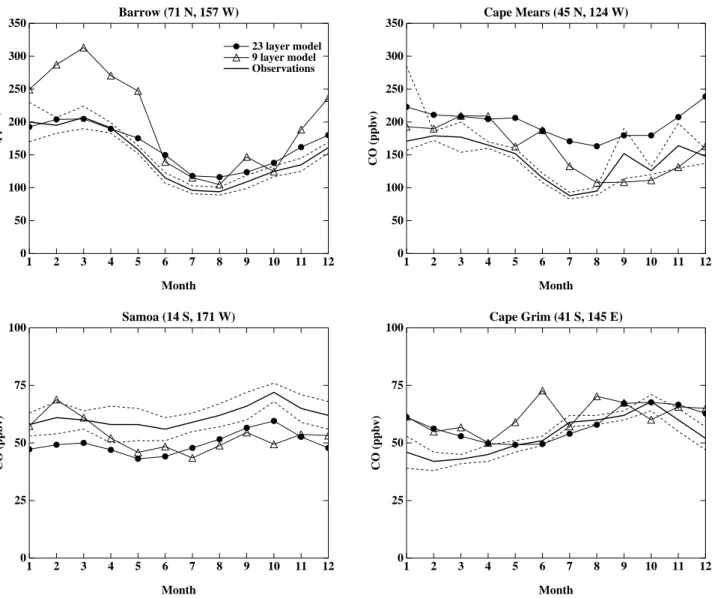
1 2 3 4 5 6 7 8 9 10 11 12 0 50 100 150 200 250 300 350 23 layer model 9 layer model Observations Barrow (71 N, 157 W) Month CO (ppbv) 1 2 3 4 5 6 7 8 9 10 11 12 0 50 100 150 200 250 300 350 Cape Mears (45 N, 124 W) Month CO (ppbv) 1 2 3 4 5 6 7 8 9 10 11 12 0 25 50 75 100 Samoa (14 S, 171 W) Month CO (ppbv) 1 2 3 4 5 6 7 8 9 10 11 12 0 25 50 75 100 Cape Grim (41 S, 145 E) Month CO (ppbv)

Fig. 5. Comparison of observed and simulated surface carbon monoxide. Solid and dotted lines indicate measured mean values and standard deviations, respectively, while solid circles and open triangles indicate mean values from the new and old models, respectively.

comparison with the 40 sites in the climatology (counting the 4 NE US sites as one) shows the model’s mean bias is +3.8 ppbv, with a bias of +0.9 ppbv in the maximum month and +8.4 in the minimum month. The large number of rural American sites (14, again counting the 4 NE sites only once) means that the large biases there during December contribute strongly to the bias in the minimum value. The new model certainly does a much better job reproducing the observations that the older 9-layer model, which we attribute both to the expanded chemistry scheme and the greater vertical resolu-tion and updated physics in the boundary layer.

The ozone budget in the new model is substantially altered from the previous version. However, we caution that this may not be a very useful indicator of the veracity of ozone simu-lations. As discussed in Shindell et al. (2001), models report widely differing budget values, yet all profess to simulate observed ozone amounts reasonably well. Furthermore, in

testing the gravity-wave drag parameterization in the GCM, we discovered that changes in the stratosphere-troposphere exchange by a factor of two are largely compensated for by adjustment of the chemical and dry deposition terms to yield almost the same ozone fields in most areas. Another exam-ple comes from comparing the 9-layer simulation with the simplified chemistry to the 23-layer model with the same chemistry. Going to the higher resolution model reduced the stratosphere-troposphere exchange by 364 Tg/yr. In compen-sation for the reduced influx, the net tropospheric chemical production increased by 378 Tg/yr, leading to an almost iden-tical ozone burden. Similarly, comparing the simulations of the 23-layer GCM using the previous, simplified chemistry and the present more complex scheme showed that the addi-tion of higher hydrocarbon families and PANs caused an in-crease in the net chemical production of ozone of 201 Tg/yr. With a similar stratosphere-troposphere exchange in these

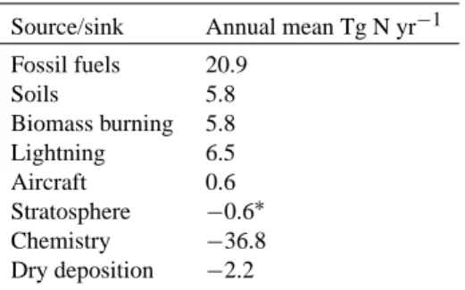
Table 4. NOxbudget

Source/sink Annual mean Tg N yr−1

Fossil fuels 20.9 Soils 5.8 Biomass burning 5.8 Lightning 6.5 Aircraft 0.6 Stratosphere −0.6∗ Chemistry −36.8 Dry deposition −2.2

∗_{The stratospheric term varies considerably between runs and with}

the choice of boundary, being the difference between the much larger upward and downward fluxes, and so is sometimes weakly positive and sometimes weakly negative.

two runs, the dry deposition increased by 191 Tg/yr, largely balancing the chemical changes and leading to an increase of only 18 Tg in the tropospheric ozone burden. Thus the system appears to be highly buffered, and since ozone is ap-proximately in steady-state in the troposphere, changes to a given factor in ozone’s budget are largely compensated for by the other terms, resulting in little net effect. Additionally, the net chemistry term is the difference between much larger production and destruction terms, so its changes can be mis-leading.

In the new model, the tropospheric ozone budget in terms of annual average fluxes (Tg/yr) is +417 stratosphere-troposphere exchange, −1466 dry deposition, and +1049 chemistry. The resulting ozone burden is 349 Tg. For comparison, the budget of the previous version was +750 stratosphere-troposphere exchange, −1140 dry deposition, +389 chemistry, and an ozone burden of 262 Tg. The val-ues for dry deposition and chemistry found here are quite large, at the high end or outside the range reported for other models. Yet the tropospheric ozone burden is in good agree-ment with the 236–364 Tg range reported by other models (Roelofs and Lelieveld, 1995; Levy et al., 1997; Roelofs et al., 1997; Houweling et al., 1998; Wang et al., 1998b; Hauglustaine et al., 1998; Mickley et al., 1999; Stevenson et al., 2000; Lelieveld and Dentener, 2000).

The stratosphere-troposphere exchange was calculated us-ing the flux across the 150 hPa surface for both the 9- and 23-layer models. Given the large gradients in the tropopause re-gion, the precise value of the exchange is sensitive to the spe-cific definition chosen. If instead we use the flux across the 250 or 60 hPa surfaces, we find values of 539 or 451 Tg/yr, respectively, in the new model. If we sum the horizontal and vertical fluxes across a surface at 300 hPa poleward of 30◦and at 100 hPa in the tropics, we find a total net flux of 342 Tg/yr. Consistent with this range, the net chemistry term over the varyingly defined troposphere ranges from 1142 to 927 Tg/yr. The stratosphere-troposphere exchange term is

the only one to have reasonably good constraints on its global value, which has been given a 450 Tg/yr best estimate with a 200–870 Tg/yr range for the cross-tropopause flux from ozone-NOy tracer correlations (Murphy and Fahey, 1994),

a value of 450–590 Tg/yr at 100 hPa based on satellite ob-servations (Gettelman et al., 1997) and 390 Tg/yr at 150 hPa (Mickley et al., 1999) based on fluxes estimated from mete-orological data (Appenzeller et al., 1996). Our comparable values are in the range of these estimates, and much better than that seen in our previous model.

If the dry deposition and chemistry were both very much too large, we might expect that although the budget would not be greatly affected since these terms oppose one another, there would be a systematic bias toward underprediction of ozone at low levels and overprediction elsewhere. The com-parison with sondes (Fig. 2 and Table 2) does not support such a bias, nor does a comparison with sonde vertical pro-files near the surface (not shown). In fact, the improvement in simulated surface ozone in polluted areas is largely at-tributable to the new planetary boundary layer scheme’s en-hancement of dry deposition. Based on the observational constraint of the surface measurements and the lowest level sonde data it appears that the faster dry deposition is more reasonable. We therefore believe that the budget is not a very useful constraint, aside from the stratosphere-troposphere ex-change term which is better constrained and also provides a useful measure of the influence stratospheric ozone on the troposphere. The key test, however, is that we have demon-strated that the model does a reasonably good job of simulat-ing observed ozone values.

3.2 Carbon monoxide

A comparison between observed and simulated annual cycles of surface carbon monoxide at several locations covering a wide range of latitudes is shown in Fig. 5. The model does a good job of matching the measured values, though there are slight positive and negative biases at Cape Mears and Samoa, respectively. Compared with the 9-layer simpler chemistry, this version does a better job of reproducing the observed seasonal cycle (especially at Barrow and Samoa), which now matches the observations fairly well at all locations, though it may be slightly underpredicted at Barrow and Cape Mears. The model has a global mean mass-weighted OH abundance of 9.7×105molecules/cm3 for the present day, matching the value of 9.4±1.3×105molecules/cm3derived from mea-surements of the lifetime of the solvent methyl chloroform (Prinn et al., 2001). The ability of the model to reproduce the mean and seasonal cycle of CO so well implies that the seasonality and amount of hydroxyl is well-simulated. Note that we have chosen to use a much reduced isoprene source in order to improve the carbon monoxide and hydroxyl sim-ulations, despite the lack of observational support for such a source strength, as in recent intercomparisons (IPCC, 2001). If we use the emission source inferred from observations, we

0 40 80 120 160 200 100 200 300 400 500 600 700 800 900 1000 Model Observed mean

Fiji (PEM Tropics B) MAR/APR

Pressure (hPa) 0 40 80 120 160 200 100 200 300 400 500 600 700 800 900 1000

Fiji (PEM Tropics A) SEP

0 40 80 120 160 200 100 200 300 400 500 600 700 800 900 1000

Japan (PEM West B) FEB/MAR

Pressure (hPa) 0 40 80 120 160 200 100 200 300 400 500 600 700 800 900 1000

Philippine Sea (PEM West B) FEB/MAR

0 200 400 600 800 1000 100 200 300 400 500 600 700 800 900 1000

E-Brazil (TRACE A) OCT

NO_x (pptv) Pressure (hPa) 0 40 80 120 160 200 100 200 300 400 500 600 700 800 900 1000

S-Atlantic (TRACE A) OCT

NO_x (pptv)

Fig. 6. Observed and simulated profiles of nitrogen oxides and nitric acid for various locations and seasons. Solid and dotted lines indicate measured mean values and standard deviations, respectively. Solid circles show mean values from the new model. Observations are taken from Emmons et al. (2000).

find the typical positive bias in CO and negative bias in OH seen in many chemical models (IPCC, 2001). It remains to be determined whether these biases result from deficiencies in current understanding of NMHC chemistry (or our

simpli-fied representation of this chemistry), in transport of emitted isoprene out of the canopy, or in some other factor.

0 200 400 600 800 1000 100 200 300 400 500 600 700 800 900 1000 Model Observed mean

Fiji (PEM Tropics B) MAR/APR

Pressure (hPa) 0 200 400 600 800 1000 100 200 300 400 500 600 700 800 900 1000

Fiji (PEM Tropics A) SEP

0 200 400 600 800 1000 100 200 300 400 500 600 700 800 900 1000

Japan (PEM West B) FEB/MAR

Pressure (hPa) 0 200 400 600 800 1000 100 200 300 400 500 600 700 800 900 1000

Philippine Sea (PEM West B) FEB/MAR

0 200 400 600 800 1000 100 200 300 400 500 600 700 800 900 1000

E-Brazil (TRACE A) OCT

HNO3 (pptv) Pressure (hPa) 0 200 400 600 800 1000 100 200 300 400 500 600 700 800 900 1000

S-Atlantic (TRACE A) OCT

HNO3 (pptv)

Fig. 6. Continued.

3.3 Nitrogen species and lightning

The budget of nitrogen oxides is shown in Table 4. We com-pare measurements of NOxand HNO3with modeled values

in Fig. 6. Observations are not available with long-term cov-erage from a fixed location as they are with ozone, so we are forced to compare with data obtained during brief field

campaigns as compiled by Emmons et al. (2000). These may not be statistically representative, however. The sample of sites shown in the figure is representative of the behavior of many additional comparisons we performed. The model generally does a good job of reproducing observed profiles of NOx. This is consistent with the model’s ability to

0 100 200 300 400 500 100 200 300 400 500 600 700 800 900 1000 Model Observed mean

Fiji (PEM Tropics B) MAR/APR

Pressure (hPa) 0 100 200 300 400 500 100 200 300 400 500 600 700 800 900 1000

Fiji (PEM Tropics A) SEP

0 200 400 600 800 1000 100 200 300 400 500 600 700 800 900 1000

Japan (PEM West B) FEB/MAR

Pressure (hPa) 0 100 200 300 400 500 100 200 300 400 500 600 700 800 900 1000

Philippine Sea (PEM West B) FEB/MAR

0 200 400 600 800 1000 100 200 300 400 500 600 700 800 900 1000

E-Brazil (TRACE A) OCT

PAN (pptv) Pressure (hPa) 0 200 400 600 800 1000 100 200 300 400 500 600 700 800 900 1000

S-Atlantic (TRACE A) OCT

PAN (pptv)

Fig. 7. Observed and simulated profiles of PANs for locations and seasons as in Fig. 6.

generating the very low values in the remote Pacific (Fig. 6). However, in a few regions, such as eastern Brazil (and south-ern Africa, not shown) the model cannot reproduce the very large values seen in the lower troposphere during the biomass burning period. Out over the South Atlantic the model gives a good match, but the continental values are too low,

sug-gesting that at least during the year of the TRACE-A obser-vations, biomass burning emissions of NOxmay have been

larger than those in our inventory. Near highly polluted areas such as Japan, the model does an excellent job of match-ing the “C-shaped” profile found in observations (Fig. 6). In contrast to NOx, the model’s simulation of HNO3 is often

JJA OTD data

DJF OTD data

JJA GCM

DJF GCM

Fig. 8. Observed and simulated distributions of lightning flash rates (flashes/km2/season). The left column shows observations from the

Optical Transient Detector satellite during 1995–1996 (other years look similar), while the right shows model results. The top row is June– August, while the bottom is December-February. Note that there are no satellite observations at high latitudes.

not in accord with observations in polluted regions. While the model mostly matches the observed profiles in the re-mote Pacific and over the Philippine Sea, it greatly over-predicts nitric acid amounts over eastern Brazil, Japan, and the South Atlantic (Fig. 6), as well as over many other lo-cations near biomass burning regions or industrialized areas (not shown). The overprediction can be a factor of 5 or so, suggesting that the discrepancy is too large to be attributed simply to coarse model resolution or emission uncertainties. An overpredicition of nitric acid is a common problem in tro-pospheric chemistry models (e.g. Wang et al., 1998b; Mick-ley et al., 1999), and likely reflects a missing removal mech-anism for nitric acid (since the NOxvalues are reasonable).

In the future, we intend to fully couple the chemistry in our model to the sulfate aerosol scheme, to consider the inclu-sion of ammonia chemistry, and to explore heterogeneous re-actions on additional surface types such as mineral aerosols and ice which may address this problem. It is also possible that the wet removal of nitric acid is underestimated, per-haps reflecting biases in model precipitation. Additionally, the GCM does not have a separate tracer for dissolved gases, so that all dissolved gases which are not removed in a given time step are returned to the gas phase, which would tend to

bias the wet removal towards lower values. This issue will also be addressed in future work.

The model’s simulation of PANs is in fairly good agree-ment with observations in many locations (Fig. 7). PANs are underpredicted over Eastern Brazil during October, consis-tent with all the nitrogen species, and there is a suggestion of a systematic overestimate in polluted regions. As with nitric acid, we are hopeful that improvement of the model’s hetero-geneous chemistry will address the latter problem. Addition-ally, our model uses a family of PANs, while the observations record only PAN itself, creating a systematic difference in the comparison.

The parameterized generation of NOxfrom lightning

pro-duces 6.5 Tg/yr N in this model. This is significantly larger than the previous model’s value of 3.9 Tg/yr, though within the expected range of 2–20 Tg/yr (WMO, 1999). The dif-ference results primarily from empirically adjusting the pa-rameterization to better match satellite observations (increas-ing the flashes per convective event coefficients for land and ocean), with smaller contributions from the altered convec-tion scheme in the new model version, and the influence of the model’s higher vertical resolution on the lightning NOx

0 1000 2000 3000 4000 5000 100 200 300 400 500 600 700 800 900 1000 Model Observed mean

Fiji (PEM Tropics B) MAR/APR

Pressure (hPa) 0 1000 2000 3000 4000 5000 100 200 300 400 500 600 700 800 900 1000

Fiji (PEM Tropics A) SEP

0 1000 2000 3000 4000 5000 100 200 300 400 500 600 700 800 900 1000

Japan (PEM West B) FEB/MAR

Pressure (hPa) 0 1000 2000 3000 4000 5000 100 200 300 400 500 600 700 800 900 1000

Philippine Sea (PEM West B) FEB/MAR

0 1000 2000 3000 4000 5000 100 200 300 400 500 600 700 800 900 1000

E-Brazil (TRACE A) OCT

H₂O₂ (pptv) Pressure (hPa) 0 1000 2000 3000 4000 5000 100 200 300 400 500 600 700 800 900 1000

S-Atlantic (TRACE A) OCT

H₂O₂ (pptv)

Fig. 9. Observed and simulated profiles of hydrogen peroxide for locations and seasons as in Fig. 6.

to that in the previous model, but is now in better agreement with Optical Transient Detector (OTD) satellite (Boccippio et al., 1998) observations (Fig. 8). The flash frequency av-eraged over all points is ∼4% greater in the GCM than in the observations, though there are underestimates over the oceans off the eastern edge of continents and over

North-ern Hemisphere middle latitudes. The older model produced flash rates ∼60–65% of those observed. This suggests that the new parameterization and convection scheme may give a more realistic overall NOxproduction from lightning.

0 500 1000 1500 100 200 300 400 500 600 700 800 900 1000 Model Observed mean

Fiji (PEM Tropics B) MAR/APR

Pressure (hPa) 0 500 1000 1500 100 200 300 400 500 600 700 800 900 1000

Fiji (PEM Tropics A) SEP

0 500 1000 1500 100 200 300 400 500 600 700 800 900 1000

Japan (PEM West B) FEB/MAR

Pressure (hPa) 0 500 1000 1500 100 200 300 400 500 600 700 800 900 1000

Philippine Sea (PEM West B) FEB/MAR

0 500 1000 1500 100 200 300 400 500 600 700 800 900 1000

E-Brazil (TRACE A) OCT

CH₃OOH (pptv) Pressure (hPa) 0 500 1000 1500 100 200 300 400 500 600 700 800 900 1000

S-Atlantic (TRACE A) OCT

CH₃OOH (pptv)

Fig. 10. Observed and simulated profiles of CH3OOH for locations and seasons as in Fig. 6.

3.4 Hydrogen peroxide and methyl hydroperoxide

The model does a generally good job reproducing observed hydrogen peroxide values in most regions regardless of sea-son (Fig. 9). In contrast to the previous model version, the model is now able to capture the huge enhancement of H2O2

in the lower troposphere over Brazil in the fall, albeit with

a somewhat reduced magnitude (as expected from the NOx

bias). The model’s simulation over southern Africa during this time of year is also improved (not shown). The model exhibits a positive bias in the region of 900 hPa over portions of the Pacific similar to that shown for Fiji during March– April, but even larger at Tahiti, Hawaii, and Christmas Is-land. Given the apparent reasonably good quality of the OH