Can fiscal rules curb income inequality? Evidence from developing countries

(1)

C E N T R E D' ÉT U D E S E T D E R E C H E R C H E S S U R L E D E V E L O P P E M E N T I N T E R N A T I O N A L

SÉRIE ÉTUDES ET DOCUMENTS

Can fiscal rules curb income inequality? Evidence from developing countries

Jean-Louis Combes

Alexandru Minea

Pegdéwendé Nestor Sawadogo

Cezara Vinturis

Études et Documents n° 25

December 2019

[First version: March 2019 ; This version: revised December 2019]

To cite this document:

Combes J.-L., Minea A., Sawadogo P. N., Vinturis C. (2019) “Can fiscal rules curb income

inequality? Evidence from developing countries”, Études et Documents, n° 25, CERDI.

CERDI POLE TERTIAIRE 26 AVENUE LÉON BLUM F-63000 CLERMONT FERRAND TEL.+33473177400 FAX +33473177428 http://cerdi.uca.fr/

(2)

2

The authors

Jean-Louis Combes

Université Clermont Auvergne, CNRS, CERDI, F-63000 Clermont-Ferrand, France.

Email address: [email protected]

Alexandru Minea

Université Clermont Auvergne, CNRS, CERDI, F-63000 Clermont-Ferrand, France, and Department of Economics, Carleton University, Canada.

Pegdéwendé Nestor Sawadogo

Université Clermont Auvergne, CNRS, CERDI, F-63000 Clermont-Ferrand, France.

Cezara Vinturis

Université Clermont Auvergne, CNRS, CERDI, F-63000 Clermont-Ferrand, France, and West University of Timisoara, Romania.

Corresponding author: Alexandru Minea

Études et Documents are available online at: https://cerdi.uca.fr/etudes-et-documents/

Director of Publication: Grégoire Rota-Graziosi

Editor: Catherine Araujo-Bonjean

Publisher: Mariannick Cornec

ISSN: 2114 - 7957

Disclaimer:

Études et Documents is a working papers series. Working Papers are not refereed, they constitute

research in progress. Responsibility for the contents and opinions expressed in the working papers rests solely with the authors. Comments and suggestions are welcome and should be addressed to the authors.

(3)

3 Abstract

Despite a large literature linking fiscal policy and income inequality (IQ), the relationship

between fiscal rules (FR) and IQ is severely underexplored. In a large panel of developing

countries, propensity score matching estimations reveal that countries that adopted FR

experience a significant decrease in their IQ with respect to countries that did not.

Economically meaningful, this favorable effect is robust to a wide set of alternative

measurement, methodology, and modeling specifications. Moreover, we unveil significant

differences among FR: balanced budget and debt rules robustly decrease IQ, contrary to

expenditure rules that increase it. Finally, the effect of FR on IQ is subject to heterogeneity

related to structural factors. Given the current global IQ trends, our results showing that the

FR are not neutral for IQ may provide insightful evidence for governments of countries aiming

at adopting FR.

Keywords

Fiscal rules, Income inequality, Developing countries, Impact analysis.

JEL Codes

(4)

I. Introduction

Income inequality (IQ) trends are periodically scrutinized by economists (see e.g. Anand and

Segal, 2008; Piketty, 2014; Alvaredo et al., 2017), probably due to the large consequences of

IQ—see e.g. Wilkinson and Pickett (2009) The Spirit Level: Why More Equal Societies

Almost Always Do Better?, Stiglitz (2012) The Price of Inequality: How Today’s Divided

Society Endangers Our Future, or Atkinson (2015) Inequality: What Can Be Done?. From a

macroeconomic perspective, the literature devoted to IQ focuses on mainly three issues.

A first strand of literature, capitalizing on the pioneering work of Kuznets (1955),

looks at the determinants of IQ; prominent determinants include international factors, such as

globalization or trade (e.g. Dollar and Kraay, 2004; Goldberg and Pavcnik, 2007; Dreher and

Gaston, 2008; Ezcurra and Rodriguez-Pose, 2013; Kanbur, 2015), financial factors (e.g.

Claessens and Perotti, 2007; Demirguc-Kunt and Levine, 2009; Kim and Lin, 2011),

technological change (e.g. Galor and Moav, 2000; Acemoglu, 2002; Jovanovic, 2009),

institutions (e.g. Chong and Gradstein, 2007; Acemoglu et al., 2015; Lin and Fu, 2016),

inflation (e.g. Romer and Romer, 1999; Bulir, 2001; Albanesi, 2007); or natural resources

(e.g. Gylfason and Zoega, 2002; Fum and Hodler, 2010; Parcero and Papyrakis, 2016).

Second, IQ is regularly pointed out as a major source of various macroeconomic

imbalances; for example, IQ is found to reduce economic growth

1

_{(e.g. Alesina and Rodrik,}

1994; Persson and Tabellini, 1994; Ostry et al., 2014; Berg et al., 2018; and possibly

contribute to the secular stagnation, see Auclert and Rognlie, 2018) or the quality of the

institutions (Alesina and Perotti, 1996), to increase inflation (Beetsma and van der Ploeg,

1996) and poverty (Ravallion, 1997), and to contribute to underdevelopment (Easterly, 2007)

and even crises, including the recent Great Recession (Rajan, 2010; Reich, 2010).

Third, given these detrimental effects, a wide variety of policies were imagined to

bring down IQ. Such policies may be related with e.g. trade (UNCTAD, 2019), FDI (Figini

and Gorg, 2011), human capital (Goldin and Katz, 2009), finance (Brei et al., 2018),

technology (UNESCAP, 2018, chapter 4), or the labor market (Berg, 2015).

Belonging to the latter strand of literature, this paper asks the following question: can

fiscal rules (FR) curb income inequality (IQ)?

2

_{Such a question is legitimate since FR affect}

1_{However, some early 2000s studies reported that IQ may sometimes increase growth (e.g. Forbes, 2000).}

2_{Nowadays, FR—defined as permanent constraints on fiscal policy, expressed in terms of a summary indicator}

of fiscal performance (Kopits and Symansky, 1998)—became a popular tool for conducting fiscal policy (in more than 90 countries according to the 2015 IMF Fiscal Rules Dataset), despite a certain lack of consensus regarding their macroeconomic performances, with mostly pros—FR may e.g. improve fiscal discipline (Debrun et al., 2008), make fiscal policy more countercyclical (Combes et al., 2017), or reduce inflation (Combes et al.,

(5)

various dimensions of the fiscal policy, which received by far the greatest attention among all

policies aiming at reducing IQ both from international institutions (e.g. OECD, 2015, chapters

3 and 7; or IMF, 2017) and academia—for recent surveys, see e.g. Bastagli et al. (2012),

Heshmati and Kim (2014), Clements et al. (2015), or Anderson et al. (2017). In light of this

literature, the potential effect of FR on IQ can transit through at least three channels.

First, and most importantly, by affecting the fiscal balance (e.g. Debrun et al., 2008;

Tapsoba, 2012; Combes et al., 2018), FR most likely influence both government spending and

revenues. While more recently e.g. Joumard et al. (2012), Martinez-Vazquez et al. (2012), or

Higgins and Lustig (2016) discuss the effect of taxes on IQ, the meta-analysis of Anderson et

al. (2017) performed on 84 studies reports mitigated findings for the government spending-IQ

link: while total government spending present a moderate positive relationship with IQ, some

types of government spending, including social or consumption spending, present a moderate

negative relationship with IQ.

Second, following the Great Recession many countries enacted FR together with fiscal

consolidation programs, in accordance with previous evidence supporting a key role of FR for

fiscal consolidations (e.g. Guichard et al., 2007). In turn, recent studies suggest that fiscal

consolidations may be associated with higher IQ particularly when based on spending cuts

(e.g. Ball et al., 2013; Woo et al., 2013; Agnello and Sousa, 2014), while the opposite may

arise for tax-based fiscal consolidations (Ciminelli et al., 2019).

Third, by affecting in particular fiscal policy cyclicality (e.g. Debrun et. al. 2008;

Bova et al., 2014; Combes et al., 2017; Guerguil et. al., 2017) and government borrowing

costs (e.g. Badinger and Reuter, 2017; Thornton and Vasilakis, 2018), FR are likely to

influence fiscal policy equally in the medium-run, for example in terms of public debt

dynamics and fiscal policy credibility. In turn, credibility may affect IQ for example through

capital flows (Jaumotte et al., 2013), while there seems to be a positive link between public

debt and IQ, particularly in OECD (e.g. Azzimonti et al., 2014; Arawatari and Ono, 2017).

To explore the relationship between FR and IQ, we draw upon the propensity

scores-matching (PSM) method that properly overcomes the selection bias related with the adoption

of FR.

3

_{We aim at estimating potential differences in IQ between countries that adopted FR}

and that did not adopt FR but present a comparable probability of adopting FR conditional on

a set of covariates, i.e. comparable propensity scores (Rosenbaum and Rubin, 1983).

3_{Initially employed in macroeconomics to analyze inflation targeting adoption (e.g. Lin and Ye, 2007; Minea}

(6)

Our analysis conducted on wide panel of 84 developing countries over the period

1990-2015 reveals the following. First, countries that adopted FR experience a significant

decrease in their IQ with respect to comparable countries that did not adopt FR. All the more

that IQ is most likely not the primary goal that motivates the adoption of FR, this favorable

effect is economically meaningful as it ranges between 18% and 30% of the standard

deviation of our measure of IQ. The strength of our finding is confirmed by a rich robustness

analysis that includes an alternative IQ measure, additional control variables, the entropy

balancing method as an alternative to the PSM method, or different samples—and in

particular the inclusion of developed countries.

Second, since not all FR are alike, we explore possible heterogeneities in their effect

on IQ. On the one hand, we find that contrary to the favorable effect of balanced budget rules

(BBR) and debt rules (DR) on IQ, the presence of expenditure rules (ER) strongly increases

IQ; a possible explanation is related to the fact that ER may constrain government expenditure

(e.g. Tapsoba, 2012; Dahan and Strawczinski, 2013), including spending that may contribute

to reduce IQ. On the other hand, when combining these rules two by two, we reveal

complementarities in the favorable effect of BBR and DR on IQ, as well as a neutralization of

the unfavorable effect of ER on IQ in the presence of BBR or DR.

Third, switching to the control function regression method, we explore possible

heterogeneities driven by various economic and structural factors in the relationship between

FR and IQ. On the one hand, considering FR altogether, we reveal that the favorable effect of

FR alone on IQ can be amplified in a context of deteriorated fiscal space (for example, a

higher public debt); when combined with FR, higher trade further supports the favorable

effect of FR on IQ; better political stability reduces IQ when combined with FR; and that

education (economic growth or mineral rents) reduces (increase) IQ when combined with FR.

On the other hand, combining various FR and various economic and structural variables

reveals additional heterogeneities. Compared with findings for all FR, the interactive effect

may become significant or—on the contrary—turn into not significant; the interactive effect

of some variables may differ across the various types of FR; and some variables may weaken

the unfavorable effect of ER on IQ illustrated in the benchmark estimations.

Consequently, in light of our analysis, the adoption of FR mostly reduces IQ.

However, not only the magnitude of this effect may vary with the precise type of FR, but

some FR—and in particular ER—are found to significantly increase IQ. In addition, the

effect of various types of FR on IQ may be subject to important heterogeneities, related to a

wide set of fiscal, monetary, international, political, or structural factors. Given the

(7)

importance of IQ in developing countries and its upward trend in many advanced countries

(see e.g. IMF, 2017), our results showing not only that FR are not neutral for IQ, but also

identifying cases in which various FR may curb or on the contrary increase IQ, may provide

insightful evidence for governments aiming at adopting FR.

The paper is organized as follows. Section 2 presents the data and the methodology,

section 3 reports our main results, section 4 assesses their robustness, section 5 investigates

the impact of various types of FR on IQ, section 6 explores heterogeneities in the effect of FR

on IQ related with various economic and structural factors, and section 7 concludes.

II. Data and methodology

2.1. Data

We explore the effect of FR on IQ using a yearly panel of 84 developing countries over the

period 1990-2015, selected mainly on two grounds. On the one hand, in the developing world

the presence of trustworthy fiscal data begins in the 1990s. On the other hand, to ensure the

comparability between the groups of FR and non-FR countries, i.e. for the control group to be

a good counterfactual for the treatment group, we exclude from the group of non-FR countries

those with a real per capita GDP lower than that of the poorest FR country, and a smaller

population than that of the smallest FR country.

Our main variables are IQ and FR. Following previous studies (e.g. Afesorgbor and

Mahadevan, 2016), we measure IQ by the Gini index of the disposable net income extracted

from the Standardized World Income Inequality Database (SWIID) developed by Solt (2016),

which provides comparable data across countries. We capture FR by a dummy variable equal

to 1 if for a given country in a given year a fiscal rule is at work and to 0 otherwise, using the

IMF Fiscal Rules Dataset. Appendix A in the Online Supplementary Material presents the list

of countries and the year of FR adoption.

2.2. Methodology

The presentation of the methodology is standard, and follows the existing work (e.g. Lin and

Ye, 2007; Tapsoba, 2012). The average treatment effect of the treated (ATT) equals the

average difference between IQ in countries that adopted FR (

FR

=

1 ), namely

IQ

1

, and the

IQ they would have had in the absence of FR, namely

IQ

0

(

)



1

−

0

=

1  

=

1

=

1  

−

0

=

1 

=

E

IQ

i

IQ

i

FR

i

E

IQ

i

FR

i

E

IQ

i

FR

i

(8)

Unfortunately, the latter term is not observable, and a solution would be to simply compare

the average IQ in countries that adopted FR and countries that did not. However, this would

lead to biased results, given that the adoption of FR (i.e. the treatment) is most likely not

random but correlated with a set of observable variables that may equally affect IQ (i.e. the

“self-section” problem, see e.g. Heckman et al., 1998, and Dehejia and Wahba, 2002).

Instead, under the conditional independence assumption (namely, conditional to a set of

observed variables

X ,

IQ

1

and

IQ

0

are independent of the FR adoption), we can replace the

last term of (1) by the IQ in countries that did not adopt FR but present comparable values of

the variables

X



IQ

i

FR

i

X

i

 

E

IQ

i

FR

i

X

i



E

ATT

=

1

=

1 ,

−

0

=

0 ,

.

(2)

Although the last term of (2) is observable, matching countries on a large set of variables

could raise practical issues. Therefore, we follow Rosenbaum and Rubin (1983), and

concentrate the information from set

X into the variable

p

Xi

=

Pr



FR

i

=

1 X

i



, which

provides, conditional on the set

X , the probability of adopting FR. Assuming, for each

country that adopted FR, the existence of comparable countries that did not adopt FR (i.e. the

common support assumption), the ATT finally rewrites as



IQ

i

FR

i

p

X_i



E



IQ

i

FR

i

p

X_i



E

ATT

=

1

=

1 ,

−

0

=

0 ,

.

(3)

When estimating (3), we follow the existing literature (e.g. Lin and Ye 2007; Minea &

Tapsoba, 2014), and draw upon a large variety of propensity scores-matching methods.

III. Results

3.1. The estimation of the propensity scores

We estimate the propensity scores using a probit model with the FR dummy as the dependent

variable. To account for macroeconomic and political factors related to the adoption of FR,

we draw upon the existing literature on FR (e.g. Debrun and Kumar, 2007; Tapsoba, 2012;

Combes et al., 2017; or Eyraud et al., 2018), and use a wide range of control variables (see

Appendix A for the description and sources of variables, and for descriptive statistics).

First, since FR are most likely to be introduced in countries with good macroeconomic

performances (e.g. IMF, 2009; Tapsoba, 2012), higher economic growth (measured by the

real GDP per capita growth) is expected to increase the probability of FR adoption. Although

the same may hold for external debt (in ratio of GDP), FR may equally be adopted to stabilize

a large indebtedness, making uncertain the overall effect of debt on the likelihood of FR

(9)

adoption. Second, given their higher demand for social spending, countries with higher

population dependency ratio will have a lower likelihood of FR adoption, facing more

difficulties to introduce fiscal discipline (Calderón and Schmidt-Hebbel, 2008). Third, as

emphasized by e.g. Kose et al. (2009), a larger capital openness (that we measure using the

Chinn and Ito, 2008, index) fosters a more efficient allocation of capital, which may stimulate

economic growth and constitute a prerequisite for the adoption of FR. Fourth, since the

adoption of inflation targeting often went along with the establishment of FR and other fiscal

reforms (e.g. fiscal responsibility laws, fiscal transparency, fiscal accountability) to ensure

fiscal discipline (e.g. Minea and Tapsoba, 2014; Combes et al., 2018), we expect a positive

link with FR adoption. At the same time, a higher inflation—measured as log(1+inflation)—

may signal a poor quality of monetary institutions, and is expected to negatively affect the

likelihood of FR. Fifth, following e.g. Tapsoba (2012), we account for political factors. On

the one hand, a high political risk usually signals poor institutions (including fiscal institutions

that should guarantee the respect of FR), and should negatively affect the probability of FR

adoption. On the other hand, since the government fractionalization may raise public spending

pressures (e.g. Perotti and Kontopoulos, 2002), voters may support the establishment of

strengthened fiscal frameworks to offset them, thereby increasing the need for FR.

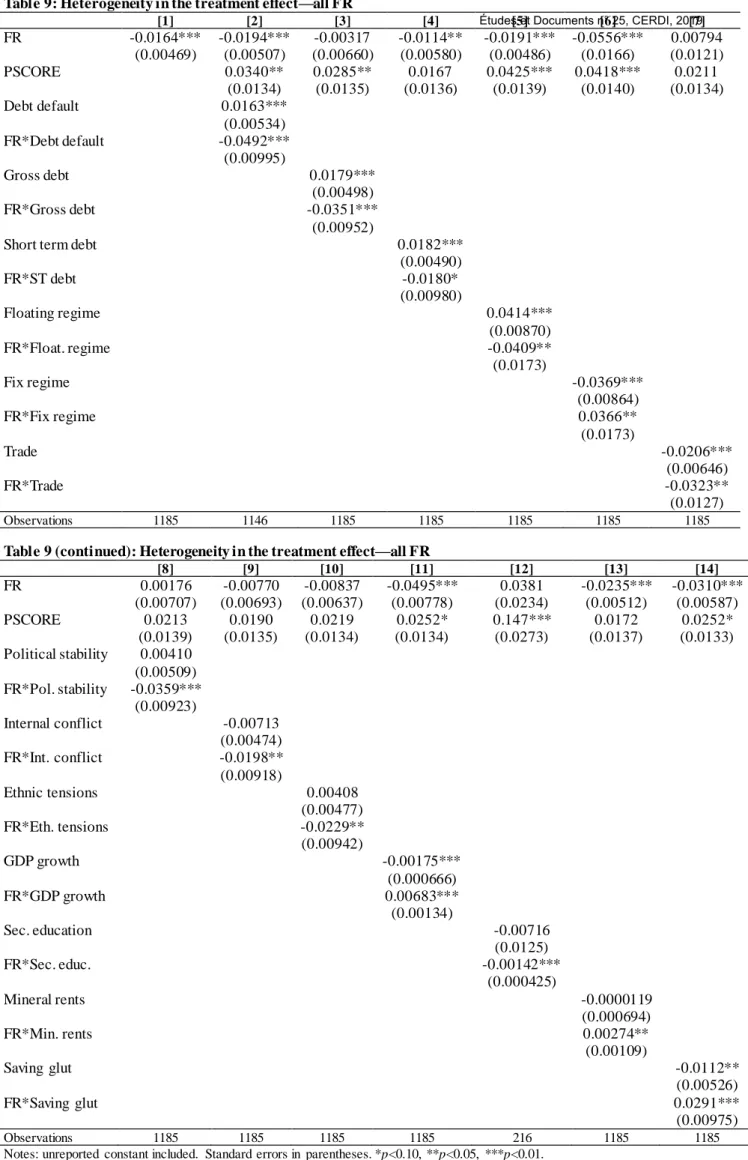
Table 1 reports the probit estimates of the PS. As shown by column [1], coefficients of

most variables are significant and confirm our expectations. Among the significant effects,

GDP per capita growth, the presence of an inflation targeting regime, and government

fractionalization increase the probability of FR adoption, with opposite effects for the

dependency ratio, inflation, and political risks.

(10)

Table 1: The estimation of propensity scores [1] [2] [3] [4] [5] [6] [7] [8] L.Real gdppc growth 0.00815* 0.00811* 0.00816* 0.00880* 0.00917* 0.0115** 0.00874* 0.00817* (0.00478) (0.00480) (0.00480) (0.00489) (0.00493) (0.00561) (0.00481) (0.00478) L.Debt 0.00154 0.00154 0.00154 0.00216* 0.00226* 0.00388*** 0.00192 0.00155 (0.00116) (0.00116) (0.00116) (0.00118) (0.00118) (0.00119) (0.00118) (0.00116) L.Dependency ratio -0.00619** -0.00619** -0.00619** -0.00667** -0.00654** -0.00685** -0.00669*** -0.00626** (0.00259) (0.00259) (0.00259) (0.00268) (0.00270) (0.00283) (0.00259) (0.00259) L.Capital openness 0.0971*** 0.0968*** 0.0971*** 0.0748** 0.0755** 0.0921*** 0.0865*** 0.0967*** (0.0292) (0.0292) (0.0292) (0.0296) (0.0296) (0.0310) (0.0290) (0.0292) L.Inflation -5.574*** -5.551*** -5.580*** -5.389*** -5.417*** -5.588*** -5.938*** -5.603*** (0.914) (0.947) (0.943) (0.915) (0.922) (1.062) (0.926) (0.917) IT_conservative 0.636*** 0.635*** 0.636*** 0.629*** 0.635*** 0.641*** 0.567*** (0.116) (0.116) (0.116) (0.118) (0.118) (0.122) (0.116) L.Political risk -0.0164*** -0.0163*** -0.0164*** -0.0159*** -0.0159*** -0.0212*** -0.0133** -0.0164*** (0.00568) (0.00569) (0.00569) (0.00572) (0.00572) (0.00600) (0.00578) (0.00568) L.Gov fractionalization 0.430*** 0.430*** 0.430*** 0.422*** 0.426*** 0.452*** 0.452*** 0.432*** (0.152) (0.152) (0.152) (0.155) (0.155) (0.159) (0.153) (0.152) Fix regime 0.0564 (0.302) Floating regime 0.0147 (0.309) CBI_regular -0.0982 (0.234) CBI_irregular 0.137 (0.124) Debt default -0.658*** (0.162) Resource-Rich 0.368*** (0.0893) IT_default 0.625*** (0.115) Observations/Pseudo-R2 1234/0.141 1234/0.141 1234/0.141 1189/0.134 1189/0.135 1151/0.170 1234/0.152 1234/0.141

(11)

3.2. The results of matching on propensity scores

Using estimated PS, we match countries that adopted FR with comparable countries that did

not, drawing upon four popular matching methods. First, the nearest-neighbor matches each

FR country with the non-FR countries with the closest PS (we retain up to

n

=

3 neighbors).

Second, the radius matches each FR with all non-FR countries with PS within a radius (we

retain a small

R

=

0 .

005 , a medium

R

=

0 .

01 , and a large

R

=

0 .

05 radius). Third, the local

linear regression (Heckman et al., 1998) matches covariates-adjusted outcomes of each FR

country with the corresponding ones of non-FR countries. Fourth, Kernel matches each FR

country with a weighted-average of all non-FR countries (weights are inversely proportional

to the gap between the PS of the FR and non-FR countries). Since the matching estimator has

no analytical variance, we compute bootstrapped standard errors (Dehejia and Wahba, 2002).

Before discussing the main results, we report that statistical tests support the quality of

our estimations. First, following Sianesi (2004), the pseudo-R2 test analyzes the common

support assumption by estimating the PS on matched and non-matched observations to

contrast their fit before and after matching. Pseudo-R2 reported in Table 2 are fairly close to

zero (i.e. always below 0.01), suggesting that the matching provided balanced scores.

Consequently, our estimations are robust with regard to the common support hypothesis.

Second, we explore the conditional independence assumption in two ways. Regarding

unobservables, the lower bound of the Rosenbaum (2002) sensitivity test, conducted at the

usual 5% significance level under the assumption of an underestimated ATT, is around 1.4

(see Table 2), comparable with existing studies (e.g. around 1.2 in Guerguil et al., 2017).

Regarding observables (see Rosenbaum, 2002), the p-values of the equality test of the mean

difference (standardized bias) between the characteristics of countries that adopted and did

not adopt FR supports the absence of statistical differences after matching (see Table 2).

Thus, estimations are equally robust with respect to the conditional independence assumption.

Given these diagnostic tests, using estimated PS from column [1] of Table 1, our

benchmark results are reported on line [1] of Table 2. Irrespective of the matching method,

the estimated ATT is negative and statistically significant: with respect to comparable

countries that did not adopt FR, countries that adopted FR experience a significant IQ

reduction. In absolute value, the estimated decrease in IQ ranges between 0.0135 (radius

01 .

0 =

r

) and 0.0217 (neighbor

n

=

2 ), depending on the retained specification. Since they

represent between 18% and 30% of the standard deviation of our IQ variable (equal to 0.073,

see Appendix A), these numbers are economically meaningful, all the more that IQ is most

likely not the primary goal that motivates the adoption of FR.

(12)

Table 2: Matching results

1-Nearest 2-Nearest 3-Nearest

Radius Matching Local Linear

Treatment Variable: FR Neighbor Neighbor Neighbor Regression Kernel

Matching Matching Matching r=0.005 r=0.01 r=0.05 Matching Matching

Dependent variable: Gini Index

[1] ATT: Differences in Inequality -0.0195** -0.0217*** -0.0211*** -0.0135** -0.0144** -0.0174*** -0.0171*** -0.0175***

(0.00916) (0.00778) (0.00731) (0.00681) (0.00615) (0.00534) (0.00540) (0.00570)

Number of observations, of which: 1192 1192 1192 1192 1192 1192 1192 1192

- treated observations 291 291 291 291 291 291 291 291

- control observations 901 901 901 901 901 901 901 901

Quality of the matching

Pseudo-R2 0.004 0.005 0.005 0.003 0.002 0.002 0.004 0.002

Rosenbaum bounds sensitivity test 1.8 1.5 1.5 1.1 1.4 1.5 1.3 1.5

Standardized bias (p-value) 0.88 0.79 0.80 0.96 0.86 0.98 0.88 0.98

(13)

IV. Robustness

This section investigates the robustness of the favorable effect of FR adoption on IQ.

4.1. An alternative measure of inequality

Our main IQ measure is the Gini index based on the net income from Solt (2016). We

consider an alternative IQ measure, from the United Nation University World Institute for

Development Economics Research (UNU-WIDER). Given data availability and for

consistency with our main measure, we focus on IQ based on equivalized household

disposable (post-tax, post-transfer) income. The results of the matching using PS from column

[1] in Table 1 are reported in Table 3. Our usual tests support the quality of the matching.

Moreover, all ATTs are negative and significant, suggesting that the decrease in IQ following

the adoption of FR does not change with the IQ measure. Finally, the estimated decrease in IQ

varies in absolute value between 0.0236 and 0.0458 (namely, between 25% and 48% of the

standard deviation), a magnitude somewhat higher compared with our benchmark findings.

4.2. Additional controls

We augment the benchmark probit model (column [1] in Table 1) with several additional

variables, namely: the exchange rate regime (we distinguish corner, i.e. fixed and floating

regimes); the central bank independence (the regular and irregular change in central banks’

governor turnover); debt default experiences; natural resources endowment (signaling

resource-rich countries); and the presence of a default (instead of a conservative) inflation

targeting regime (Appendix A provides definitions, sources, and descriptive statistics).

According to columns [2]-[8] in Table 1, most additional variables do not have a

significant effect, confirming the robustness of our benchmark model. Whenever significant,

their effect is consistent with what one may expect; in particular, countries with a history of

debt default are less likely to adopt FR, which requires fiscal institutions inconsistent with

default, while being a resource-rich country may generate additional fiscal revenues that relax

the government’s budget constraint and may support its capacity to respect the FR.

Based on PS computed using Table 1, lines [1]-[7] in Table 4 report the ATT.

Corroborating our benchmark results, the ATTs are significant and negative irrespective of

the considered specification. In addition, the size of the effect is equally consistent with our

benchmark findings, ranging (in absolute value) between 0.0140 (neighbor

n

=

1 , line [5]) and

0.0257 (neighbor

n

=

1 , line [7]). Overall, accounting for additional control variables confirms

the significant reduction of IQ in countries that adopted FR.

(14)

Table 3: Matching results: Robustness—Inequality measured using the UNU-WIDER database

[1] ATT: Differences in Inequality -0.0427*** -0.0362** -0.0305** -0.0458*** -0.0378*** -0.0236** -0.0250** -0.0244**

(0.0162) (0.0145) (0.0141) (0.0161) (0.0143) (0.0115) (0.0121) (0.0116)

Observations/treated observations 447/125

Pseudo-R2 0.02 0.02 0.02 0.01 0.01 0.01 0.02 0.01

Rosenbaum bounds sensitivity test 1.7 1.6 1.4 2 1.8 1.4 1.5 1.5

Note: standard errors in parentheses. *p<0.10, **p<0.05, ***p<0.01.

Table 4: Matching results: Robustness—Additional controls

ATT: Differences in Inequality Matching Matching Matching r=0.005 r=0.01 r=0.05 Matching Matching

Robustness checks

[1] Adding Fix exchange regime -0.0206** -0.0156** -0.0173** -0.0186*** -0.0165*** -0.0171*** -0.0167*** -0.0170***

(0.00853) (0.00791) (0.00718) (0.00691) (0.00591) (0.00511) (0.00549) (0.00538)

[2] Adding Floating exchange regime -0.0197** -0.0164** -0.0188*** -0.0179*** -0.0165*** -0.0158*** -0.0158*** -0.0156***

(0.00870) (0.00767) (0.00713) (0.00643) (0.00611) (0.00566) (0.00536) (0.00549)

[3] Adding CBI regular turnover -0.0163* -0.0185** -0.0162** -0.0190*** -0.0179*** -0.0183*** -0.0186*** -0.0185***

(0.00922) (0.00815) (0.00766) (0.00678) (0.00618) (0.00551) (0.00548) (0.00577)

[4] Adding CBI irregular turnover -0.0169* -0.0162** -0.0167** -0.0184*** -0.0165*** -0.0172*** -0.0179*** -0.0170***

(0.00874) (0.00752) (0.00726) (0.00679) (0.00621) (0.00558) (0.00548) (0.00558)

[5] Adding Debt default dummy -0.0140* -0.0146* -0.0143** -0.0180*** -0.0166*** -0.0172*** -0.0176*** -0.0173***

(0.00848) (0.00750) (0.00721) (0.00656) (0.00627) (0.00554) (0.00505) (0.00539)

[6] Adding Resource-Rich country dummy -0.0249*** -0.0192** -0.0221*** -0.0245*** -0.0223*** -0.0248*** -0.0254*** -0.0247***

(0.00963) (0.00888) (0.00780) (0.00737) (0.00670) (0.00625) (0.00622) (0.00615)

[7] Using IT Default date -0.0257*** -0.0220*** -0.0186*** -0.0161** -0.0169*** -0.0171*** -0.0169*** -0.0171***

(0.00848) (0.00757) (0.00714) (0.00646) (0.00628) (0.00534) (0.00563) (0.00529)

(15)

4.3. An alternative estimation method

To check if our main results based on PSM still hold when using an alternative technique, we

draw upon the entropy balancing method of Hainmueller (2012)—see Neuenkirch and

Neumeier (2016) and Balima et al. (2018) for a presentation of the method. Table 5a shows

that a simple comparison of main control variables’ averages in countries that adopted FR

(column [1]) and that did not adopt FR (column [2]) reveals statistically-significant

differences for almost all variables (column [4]). To neutralize the potential influence of such

differences on the treatment effect, we compute a synthetic control group by applying weights

to non-FR observations such as the average of variables in this group (column [5]) is not

statistically different from their average in the FR group (column [2]), as in column [7].

Table 5a: Building the synthetic control group

[1] [2] [3]=[1]-[2] [4] [5] [6]=[5]-[2] [7]

Variables Non-FR FR difference p_value W_Non-FR difference p_value

L.real gdppc growth -7.427 2.319 -9.746 0.000 2.963 0.644 0.738 L.debt 60.867 53.697 7.17 0.034 56.32 2.623 0.873 L.dependency ratio 70.262 66.65 3.611 0.001 66.69 0.04 0.882 L.capital openness -.248 .05 -.297 0.000 .151 0.101 0.928 L.inflation .166 .047 .118 0.000 .0510 0.004 0.347 IT_conservative .058 .226 -.168 0.000 .266 0.04 0.889 L.political risk 60.769 62.652 -1.883 0.001 62.439 -0.213 0.898 L.gov fractionalization .195 .263 -.069 0.000 .273 0.01 0.955 Observations 807 285 285

Table 5b: Robustness—Entropy balancing estimations

[1] [2] [3] [4] [5] [6] [7] [8] Baseline (Only FR) Country-FE (CFE) Time-FE (TFE)

CFE & TFE (CTFE) Main Controls (MC) MC and CFE MC and TFE MC and CTFE FR -0.0162*** -0.0116*** -0.0122*** -0.0069*** -0.0170*** -0.0097*** -0.0074* -0.0069*** (0.00420) (0.00208) (0.00442) (0.00235) (0.00385) (0.00218) (0.00399) (0.00242) Obs. 1142

Note: Unreported constant included. Standard errors in parentheses. *p<0.10, **p<0.05, ***p<0.01.

Using these weights, Table 5b reports weighted least squares estimations. Column [1]

shows that countries that adopted FR present significantly lower IQ with respect to

comparable countries that did not adopt FR (and the magnitude of the estimated coefficient is

close to our findings based on the PSM method). Next, we take advantage of the possibility of

modeling the panel dimension with the entropy balancing method, and include country-fixed

effects (CFE), time-fixed effects (TFE), and both CFE and TFE. According to columns

[2]-[4], the decrease of IQ remains significant in the presence of fixed effects. Moreover, a

significant effect is still at work when we add in column [5] the set of eight main control

variables used in our PSM benchmark estimation. Finally, comparable results arise when

(16)

combining the main control variables with different fixed effects in columns [6] -[8].

Consequently, the use of an alternative method, i.e. entropy balancing, allowing controlling

for unobservables through both country and time fixed effects confirms our previous

conclusion based on the PSM of a favorable impact of FR on IQ.

4.4. Alternative samples

We now look at the robustness of our benchmark findings when changing the sample. First,

we drop former Soviet Union countries due to their particular structural characteristics.

Second, we abstract of post-Cold War years (1990-1995) during which many countries

experienced particular dynamics of their economies. Third, we look if our results still hold

when abstracting of fuel exporter countries. Fourth, we drop hyperinflation episodes, defined

by annual inflation rates above 40%. Fifth, we ignore the recent financial crisis years

(2008-2009). Sixth, we extend our sample to include the group of developed countries. As illustrated

by ATTs reported on lines [1]-[6] in Table 6a, the effect of FR adoption on IQ is significant

and in some cases of a higher magnitude compared with our benchmark findings. In addition,

Table 6b shows that these results remain robust in the presence of additional control variables,

since at least 6 out of 8 ATTs are significant (at least at the 10% significance level) in each set

of estimated ATTs (i.e. except for two sets when dropping post-Cold War years), namely in

40 out of the 42 sets of estimated ATTs.

4

_{Altogether, these results support the robustness of}

our main findings.

(17)

Table 6a: Matching results: Robustness—Alternative samples

ATT: Differences in Inequality Matching Matching Matching r=0.005 r=0.01 r=0.05 Matching Matching

[1] Dropping former Soviet Union countries -0.0195** -0.0173** -0.0166** -0.0166** -0.0184*** -0.0227*** -0.0233*** -0.0228***

(0.00877) (0.00822) (0.00734) (0.00692) (0.00680) (0.00574) (0.00580) (0.00582)

[2] Dropping post-Cold War years -0.0150* -0.0148* -0.0143* -0.0138** -0.0134** -0.0100* -0.0112** -0.0101*

(0.00856) (0.00827) (0.00764) (0.00667) (0.00624) (0.00528) (0.00560) (0.00557)

[3] Dropping fuel exporters countries -0.0252*** -0.0221*** -0.0267*** -0.0279*** -0.0247*** -0.0235*** -0.0242*** -0.0236***

(0.00879) (0.00770) (0.00769) (0.00692) (0.00630) (0.00559) (0.00530) (0.00563)

[4] Dropping hyperinflation countries -0.0119 -0.0152* -0.0173** -0.0159** -0.0162*** -0.0156*** -0.0157*** -0.0158***

(0.00878) (0.00788) (0.00743) (0.00640) (0.00612) (0.00567) (0.00558) (0.00529)

[5] Dropping financial crisis years -0.0198** -0.0182** -0.0173** -0.0188*** -0.0157** -0.0176*** -0.0177*** -0.0179***

(0.00996) (0.00870) (0.00796) (0.00722) (0.00694) (0.00654) (0.00606) (0.00612)

[6] Including developed countries -0.0392*** -0.0406*** -0.0434*** -0.0396*** -0.0382*** -0.0359*** -0.0354*** -0.0361***

(0.0130) (0.0126) (0.0121) (0.00734) (0.00856) (0.00963) (0.0106) (0.00980)

Note: standard errors in parentheses. *p<0.10, **p<0.05, ***p<0.01.

Table 6b: Matching results: Robustness—Alternative samples & Additional Controls

Fix Floating CBI CBI Debt Resource IT

Treatment Variable: FR Exchange Exchange Regular Irregular Default Rich Default

Number of significant ATT coefficients (out of 8) Regime Regime Turnover Turnover Dummy Countries Dummy

[1] Dropping former Soviet Union countries 8 8 8 8 8 8 8

[2] Dropping post-Cold War years 2 1 6 6 7 8 7

[3] Dropping fuel exporters countries 8 8 8 8 8 8 8

[4] Dropping hyperinflation countries 7 8 8 7 7 8 6

[5] Dropping financial crisis years 6 8 8 7 8 8 7

[6] Including developed countries 8 8 8 8 8 8 8

(18)

V. Heterogeneity: the type of fiscal rule

The previous section confirmed that the favorable effect of FR adoption on IQ is robust. We

now investigate possible sources of heterogeneity in this effect, related to the type of fiscal

rule (this section), and the economic and structural environment (the next section).

As previously emphasized, the effect of FR on IQ transits through the way they affect

government spending and revenues, fiscal consolidations, and fiscal aggregates. However,

these variables may be affected in different ways by different FR; for example, according to

e.g. Tapsoba (2012) or Combes et al. (2018), fiscal aggregates may respond differently in the

presence of balanced budget rules (BBR), debt rules (DR), or expenditure rules (ER).

Therefore, we look in the following if the effect of FR on IQ differs among these FR.

5

5.1. Balanced budget rules (BBR)

Usually defined in relation with the overall balance, the structural balance, or the balance

“over the cycle”, BBR are aimed to ensure a sound and sustainable public finance by setting a

numerical ceiling or target on the government budget balance.

6

_{Using the dummy variable}

BBR equal to 1 if a country has a BBR and to 0 otherwise, based on PS from Table C1a in

Appendix C we report the ATT in Table 7a. ATTs are significant irrespective of the matching

method, and the favorable effect on IQ is estimated to be up to -0.0214 (neighbor

n

=

2 ).

We assess the robustness of these findings using the additional control variables from

our benchmark analysis. All ATT in lines [2]-[8] in Table 7a are significant and, consistent

with results on line [1], IQ decreases by up to 0.0294 (neighbor

n

=

1 , line [8]). Consequently,

the favorable effect of BBR on IQ is slightly stronger (in absolute value) compared with that

of all FR taken together. A possible explanation is that BBR may not affect total government

spending (e.g. Dahan & Strawczinski, 2013) but mainly public investment (e.g. Guerguil et

al., 2017), possibly leaving more room for spending that may be used to reduce IQ.

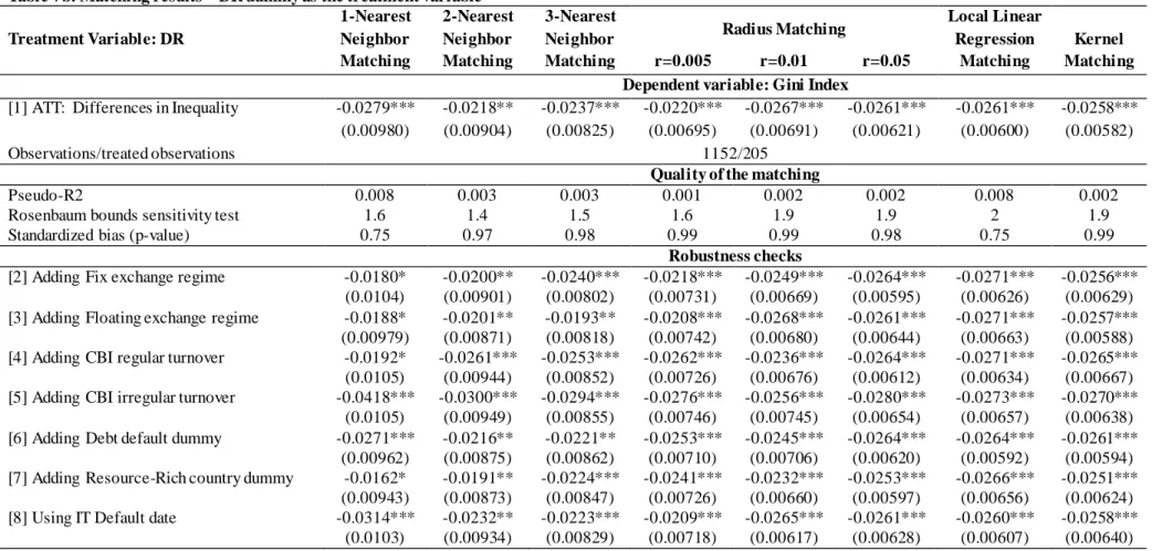
5.2. Debt rules (DR)

By setting an explicit limit on the stock of public debt (for example, the 60% debt/GDP

ceiling of the SGP), DR are designed to ensure the convergence to a debt target. Although DR

should provide an easy-to-communicate anchor to debt sustainability, they do not ensure a

clear short-run operational guidance for policymakers. While BBR and ER are more dominant

5_{The low number of countries that adopted revenue rules does not allow investigating their impact.}

6_{Examples of BBRs include (see e.g. IMF, 2009) the well-known 3% deficit-to-GDP ratio rule embodied in the}

Stability and Growth Pact (SGP); limits on structural deficits in line with the “fiscal compact” for EU countries; or the “over-the-cycle” rule that targets the average budget balance over the cycle (e.g. the UK).

(19)

in advanced and emerging countries, DR are the prevailing national rules in low-income

countries (Schaechter et al., 2012).

7

_{Based on estimated PS (see Table C1b in Appendix C),}

line [1] in Table 7b reports the ATT. Similar to BBR, all eight ATTs are significant, but the

size of the decrease in IQ is higher compared with BBR (up to -0.0279, neighbor

n

=

1 ).

These strong effects are confirmed when accounting for additional variables in lines

[2]-[8] of Table 7b: all estimated ATT are significant, and the favorable effect of DR on IQ is

reinforced, namely up to -0.0418 (neighbor

n

=

1 , line [5]). Consequently, the effect of DR on

IQ is of a stronger magnitude than that of BBR or all FR together. This may be because even

if DR place a limit on public finance, this limit is ultimately not that tight and may leave

enough room for public spending that are favorable for reducing IQ, while still providing an

anchor for reducing the probability of fiscal consolidations that may be detrimental for IQ.

5.3. Expenditure rules (ER)

ER are aimed to limit the total, primary, or current spending, by setting a ceiling on their

growth rate or as a ratio of GDP. The most important feature of ER is that they can directly

target the government size (Schaechter et al., 2012).

8

_{Using the dummy variable ER, equal to}

1 for countries that have adopted ER and to 0 otherwise, we use PS (from Table C1c in

Appendix C) to estimate the ATT of ER adoption on IQ in Table 7c. Contrary to results for all

FR, BBR, and DR, the positive (and significant in 7 out of 8 cases) ATTs suggesting that ER

adoption increases IQ. The magnitude of this effect is fairly strong, between 0.0359 (neighbor

1 .

0 =

n

) and 0.0413 (Kernel matching).

When accounting for additional variables, ATTs in Table 7c are significant in at least

5 out of 8 cases for each of the lines [2]-[8] (except on line [7]), and the detrimental effect of

ER adoption on IQ may climb up to almost 0.06 (neighbor

n

=

1 , line [3]). This harmful

impact may be related to the fact that, not only ER do not affect taxes (which may be

increased under BBR or DR, with favorable effects on IQ in the presence of progressive

taxes), but they directly constrain government spending (Tapsoba, 2012), whose reduction

may directly affect spending designed to reduce IQ.

7_{To balance flexibility and sustainability, some countries (e.g. Mauritius) included formal escape clause}

provisions that allow for temporary deviations from their debt rule. Furthermore, to avoid missing the target, some countries (e.g. Slovakia) include automatic correction mechanisms that take effect when the debt -to -GDP ratio reaches a certain level below the target.

8_{Examples of ER include a nominal expenditure ceiling for the central government (e.g. Sweden), or public}

(20)

Table 7a: Matching results—BBR dummy as the treatment variable

Treatment Variable: BBR Neighbor Neighbor Neighbor Regression Kernel

[1] ATT: Differences in Inequality -0.0183** -0.0214*** -0.0205*** -0.0210*** -0.0196*** -0.0195*** -0.0201*** -0.0195***

(0.00878) (0.00763) (0.00720) (0.00588) (0.00561) (0.00536) (0.00526) (0.00507)

Pseudo-R2 0.006 0.006 0.005 0.001 0.001 0.001 0.006 0.001

[2] Adding Fix exchange regime -0.0189** -0.0233*** -0.0240*** -0.0204*** -0.0202*** -0.0196*** -0.0201*** -0.0196***

(0.00926) (0.00821) (0.00750) (0.00652) (0.00537) (0.00501) (0.00550) (0.00512)

[3] Adding Floating exchange regime -0.0156* -0.0164** -0.0202*** -0.0202*** -0.0204*** -0.0196*** -0.0201*** -0.0196***

(0.00855) (0.00753) (0.00735) (0.00606) (0.00554) (0.00548) (0.00539) (0.00511)

[4] Adding CBI regular turnover -0.0200** -0.0233*** -0.0224*** -0.0219*** -0.0217*** -0.0199*** -0.0212*** -0.0202***

(0.00865) (0.00775) (0.00748) (0.00579) (0.00580) (0.00517) (0.00545) (0.00569)

[5] Adding CBI irregular turnover -0.0157* -0.0163** -0.0184** -0.0198*** -0.0213*** -0.0210*** -0.0219*** -0.0211***

(0.00952) (0.00774) (0.00725) (0.00623) (0.00592) (0.00529) (0.00526) (0.00533)

[6] Adding Debt default dummy -0.0247*** -0.0239*** -0.0207*** -0.0216*** -0.0217*** -0.0214*** -0.0212*** -0.0212***

(0.00859) (0.00761) (0.00703) (0.00650) (0.00550) (0.00529) (0.00507) (0.00532)

[7] Adding Resource-Rich country dummy -0.0261*** -0.0220*** -0.0257*** -0.0285*** -0.0277*** -0.0249*** -0.0259*** -0.0253***

(0.00895) (0.00836) (0.00835) (0.00689) (0.00642) (0.00624) (0.00680) (0.00639)

[8] Using IT Default date -0.0294*** -0.0277*** -0.0230*** -0.0186*** -0.0197*** -0.0194*** -0.0201*** -0.0195***

(0.00828) (0.00802) (0.00705) (0.00594) (0.00552) (0.00547) (0.00530) (0.00503)

(21)

Table 7b: Matching results—DR dummy as the treatment variable

Treatment Variable: DR Neighbor Neighbor Neighbor Regression Kernel

[1] ATT: Differences in Inequality -0.0279*** -0.0218** -0.0237*** -0.0220*** -0.0267*** -0.0261*** -0.0261*** -0.0258***

(0.00980) (0.00904) (0.00825) (0.00695) (0.00691) (0.00621) (0.00600) (0.00582)

Pseudo-R2 0.008 0.003 0.003 0.001 0.002 0.002 0.008 0.002

Rosenbaum bounds sensitivity test 1.6 1.4 1.5 1.6 1.9 1.9 2 1.9

[2] Adding Fix exchange regime -0.0180* -0.0200** -0.0240*** -0.0218*** -0.0249*** -0.0264*** -0.0271*** -0.0256***

(0.0104) (0.00901) (0.00802) (0.00731) (0.00669) (0.00595) (0.00626) (0.00629)

[3] Adding Floating exchange regime -0.0188* -0.0201** -0.0193** -0.0208*** -0.0268*** -0.0261*** -0.0271*** -0.0257***

(0.00979) (0.00871) (0.00818) (0.00742) (0.00680) (0.00644) (0.00663) (0.00588)

[4] Adding CBI regular turnover -0.0192* -0.0261*** -0.0253*** -0.0262*** -0.0236*** -0.0264*** -0.0271*** -0.0265***

(0.0105) (0.00944) (0.00852) (0.00726) (0.00676) (0.00612) (0.00634) (0.00667)

[5] Adding CBI irregular turnover -0.0418*** -0.0300*** -0.0294*** -0.0276*** -0.0256*** -0.0280*** -0.0273*** -0.0270***

(0.0105) (0.00949) (0.00855) (0.00746) (0.00745) (0.00654) (0.00657) (0.00638)

[6] Adding Debt default dummy -0.0271*** -0.0216** -0.0221** -0.0253*** -0.0245*** -0.0264*** -0.0264*** -0.0261***

(0.00962) (0.00875) (0.00862) (0.00710) (0.00706) (0.00620) (0.00592) (0.00594)

[7] Adding Resource-Rich country dummy -0.0162* -0.0191** -0.0224*** -0.0241*** -0.0232*** -0.0253*** -0.0266*** -0.0251***

(0.00943) (0.00873) (0.00847) (0.00726) (0.00660) (0.00597) (0.00656) (0.00624)

[8] Using IT Default date -0.0314*** -0.0232** -0.0223*** -0.0209*** -0.0265*** -0.0261*** -0.0260*** -0.0258***

(0.0103) (0.00934) (0.00829) (0.00718) (0.00617) (0.00628) (0.00607) (0.00640)

(22)

Table 7c: Matching results—ER dummy as the treatment variable

Treatment Variable: ER Neighbor Neighbor Neighbor Regression Kernel

[1] ATT: Differences in Inequality 0.0362* 0.0362* 0.0359** 0.0241 0.0405** 0.0412*** 0.0365** 0.0413**

(0.0194) (0.0197) (0.0183) (0.0268) (0.0203) (0.0154) (0.0150) (0.0169)

Pseudo-R2 0.10 0.06 0.04 0.008 0.03 0.03 0.10 0.03

[2] Adding Fix exchange regime 0.0507** 0.0446** 0.0426** 0.0193 0.0226 0.0437*** 0.0388** 0.0436***

(0.0211) (0.0203) (0.0185) (0.0248) (0.0216) (0.0152) (0.0160) (0.0149)

[3] Adding Floating exchange regime 0.0597*** 0.0418** 0.0430** 0.00268 0.0224 0.0435*** 0.0385*** 0.0438***

(0.0212) (0.0193) (0.0173) (0.0271) (0.0225) (0.0162) (0.0146) (0.0161)

[4] Adding CBI regular turnover 0.0409 0.0539*** 0.0528*** 0.00899 0.0253 0.0479*** 0.0457*** 0.0489***

(0.0252) (0.0208) (0.0193) (0.0303) (0.0251) (0.0177) (0.0159) (0.0170)

[5] Adding CBI irregular turnover 0.0491** 0.0436** 0.0412** -0.0106 0.0125 0.0484*** 0.0437*** 0.0450**

(0.0249) (0.0214) (0.0190) (0.0282) (0.0221) (0.0171) (0.0163) (0.0178)

[6] Adding Debt default dummy 0.0430** 0.0474** 0.0447*** 0.0347 0.0340 0.0446*** 0.0439*** 0.0445***

(0.0214) (0.0191) (0.0161) (0.0282) (0.0231) (0.0154) (0.0154) (0.0150)

[7] Adding Resource-Rich country dummy 0.0462* 0.0413* 0.0313 -0.0152 0.000196 0.0297 0.0342* 0.0278

(0.0276) (0.0234) (0.0215) (0.0264) (0.0224) (0.0197) (0.0190) (0.0189)

[8] Using IT Default date 0.0497** 0.0383* 0.0401** 0.0299 0.0393* 0.0410** 0.0364** 0.0419***

(0.0239) (0.0196) (0.0174) (0.0262) (0.0210) (0.0169) (0.0146) (0.0142)

(23)

5.4. Combined types of fiscal rules

The trend of the last decade is for countries to adopt multiple FR, and particularly combine

BBR with DR or ER (Eyraud et al., 2018). We analyze such combined effects of our three FR

on IQ using three combinations of two rules (considering all three rules together leads to too

few—eleven—treated observations for robust statistical inference). In each case, the treatment

variable is a dummy variable equal to 1 if both rules are adopted, and to 0 if not (i.e. if none

or only one rule is adopted). Matching results in Table 8 show the following.

First, the joint presence of BBR and DR significantly reduces IQ (line [1]), confirming

individual results for BBR and DR. The magnitude of this favorable effect is slightly stronger

than that of BBR or DR alone (up to -0.0312), suggesting some complementarities between

them for reducing IQ. Second, the joint effect of DR and ER is not significant (line [2]),

which may reproduce the conflicting effects of DR alone (decrease) and ER alone (increase)

on IQ. Third, the joint influence of BBR and ER is equally mostly not significant (line [3]),

reflecting yet again the conflicting effects of BBR and ER alone.

Altogether, these results (which are robust in the presence of additional control

variables in Tables C2a-b-c in Appendix C) show that combining different FR should be done

with caution in terms of IQ. On the one hand, the detrimental effect of ER adoption on IQ can

be neutralized by the presence of either BBR or DR; and the presence of both BBR and DR

reduces IQ by more compared to their individual effect. However, on the other hand, the

adoption of ER reduces the favorable effects of BBR or DR alone.

(24)

Table 8: Matching results—combined types of FR

Neighbor Neighbor Neighbor Regression Kernel

Dependent variable: Gini index

Treatment Variable: BBR*DR Dummy -0.0231** -0.0312*** -0.0295*** -0.0275*** -0.0260*** -0.0242*** -0.0226*** -0.0239***

[1] ATT: Differences in Inequality (0.0108) (0.00987) (0.00898) (0.00755) (0.00823) (0.00743) (0.00706) (0.00660)

Treatment Variable: DR*ER Dummy -0.0359 -0.0130 -0.00410 0.00159 -0.00368 -0.000283 0.00316 0.00121

Treatment Variable: BBR*ER Dummy 0.0530 0.0625* 0.0517 -0.0152 0.0168 0.0592* 0.0464 0.0576*

(25)

VI. Heterogeneity: different economic and structural environments

The previous section revealed that the effect of FR adoption on IQ varies with the type of FR.

At the same time, to account for possible differences among the countries in our sample, we

consider a large set of potential sources of heterogeneity related to fiscal, monetary,

international, political, and other structural variables. We explore such heterogeneities using a

control function regression approach (e.g. Tapsoba, 2012)

it it it it it it it

FR

PScore

X

FR

X

IQ

=



+



+



+



+



+



,

(4)

with PScore the estimated PS from the benchmark model, and X the vector of variables that

may be a source of heterogeneity. A significant coefficient of interest



signals the presence

of heterogeneity in the treatment effect. We look at all FR together and then at each rule.

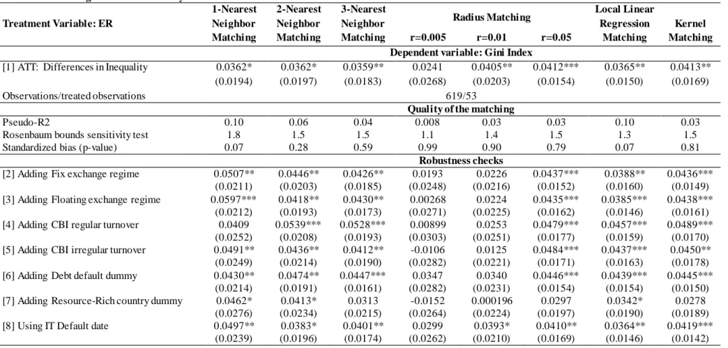
6.1. All fiscal rules

Column [1] in Table 9 shows that FR significantly decrease IQ on average by 0.0164,

comparable with our benchmark results. From column [2] onwards we report only estimations

in which the interactive effect between the considered variables and FR (i.e. the coefficient



) is significant at least at the 10% significance level.

First, columns [2]-[4] show that all fiscal variables significantly reduce IQ when

combined with FR, suggesting that the favorable effects of FR on IQ may be amplified when

FR are in place in a deteriorated fiscal space. Second, regarding monetary variables, columns

[5]-[6] reveal that the favorable effect of FR alone on IQ is enforced in the presence of

floating exchange rates (while mitigated under fixed exchange rates), suggesting that floating

exchange rates may better absorb various types of shocks that could lower the favorable effect

of FR on IQ. Third, among international variables, higher trade combined with FR

significantly reduces IQ (column [7]), as access to international markets for goods and

services may foster the efficiency of spending designed to reduce IQ within FR-based fiscal

policy frameworks. Fourth, all political environment variables, namely the degree of political

stability, the absence of internal conflicts, and the absence of ethnic tensions, reduce IQ when

combined with FR (columns [8]-[10]), possibly because better political conditions may

support more stable fiscal institutions in which the compliance with FR can be combined with

more judicious spending policies, including in terms of distributional goals.

(26)

(0.00469) (0.00507) (0.00660) (0.00580) (0.00486) (0.0166) (0.0121) PSCORE 0.0340** 0.0285** 0.0167 0.0425*** 0.0418*** 0.0211 (0.0134) (0.0135) (0.0136) (0.0139) (0.0140) (0.0134) Debt default 0.0163*** (0.00534) FR*Debt default -0.0492*** (0.00995) Gross debt 0.0179*** (0.00498) FR*Gross debt -0.0351*** (0.00952)

Short term debt 0.0182***

(0.00490) FR*ST debt -0.0180* (0.00980) Floating regime 0.0414*** (0.00870) FR*Float. regime -0.0409** (0.0173) Fix regime -0.0369*** (0.00864) FR*Fix regime 0.0366** (0.0173) Trade -0.0206*** (0.00646) FR*Trade -0.0323** (0.0127) Observations 1185 1146 1185 1185 1185 1185 1185

Table 9 (continued): Heterogeneity in the treatment effect—all FR

[8] [9] [10] [11] [12] [13] [14] FR 0.00176 -0.00770 -0.00837 -0.0495*** 0.0381 -0.0235*** -0.0310*** (0.00707) (0.00693) (0.00637) (0.00778) (0.0234) (0.00512) (0.00587) PSCORE 0.0213 0.0190 0.0219 0.0252* 0.147*** 0.0172 0.0252* (0.0139) (0.0135) (0.0134) (0.0134) (0.0273) (0.0137) (0.0133) Political stability 0.00410 (0.00509) FR*Pol. stability -0.0359*** (0.00923) Internal conflict -0.00713 (0.00474) FR*Int. conflict -0.0198** (0.00918) Ethnic tensions 0.00408 (0.00477) FR*Eth. tensions -0.0229** (0.00942) GDP growth -0.00175*** (0.000666) FR*GDP growth 0.00683*** (0.00134) Sec. education -0.00716 (0.0125) FR*Sec. educ. -0.00142*** (0.000425) Mineral rents -0.0000119 (0.000694) FR*Min. rents 0.00274** (0.00109) Saving glut -0.0112** (0.00526) FR*Saving glut 0.0291*** (0.00975)

(27)

Finally, our last set of variables captures other structural characteristics. Column [11]

shows that higher economic growth mitigates the favorable effect of FR on IQ, to the point

where above a certain growth rate FR increase IQ probably due to poor redistribution. Next,

despite relatively few available observations, education is found to reduce IQ when combined

with FR (column [12]), since a more educated population could sustain government policies

incorporating public spending designed for combating IQ. Moreover, the interactive term

between mineral rents and FR is positive (column [13]), suggesting that in our sample of

developing countries important mineral rents may increase IQ when combined with FR,

possibly echoing the famous “Dutch disease”. Lastly, column [14] indicates that the favorable

effect of FR on IQ was mitigated during the saving glut (2000-06), possibly due to a shortage

of public spending aimed at reducing IQ.

6.2. Different types of fiscal rules

We now look at heterogeneities for each type of FR. To save space, Table 10 reports only the

coefficient of the interactive term between each variable and each FR, namely significant (at

least at the 10% level) & positive (+), significant & negative (–), or not significant (NS).

Table 10. Heterogeneity by type of fiscal rule

[1] [2] [3] [4]

All FR BBR DR ER

Fiscal variables

Debt default – – NS NS

Gross debt – – NS –

Short term debt – NS – –

Government size NS – – NS Monetary variables Inflation rate NS NS NS NS Broad money NS + + – Floating regime – NS + + Fix regime + NS – – International variables Trade – NS NS – FDI Inflows NS NS NS NS Capital openness NS NS NS – Political variables Political stability – – NS – Internal conflict – NS NS – Ethnic tensions – NS – NS

Other structural variables

Growth rate of GDP + + + + Secondary education – – – – Mineral rents + + – + Post crisis NS NS NS – Saving glut + + NS + Time NS NS NS +

Note: the interaction term between each variable and the corresponding type of fiscal rule can be +, –, or NS, namely significant (at least at the 10% level) & positive, significantly & negative, and not significant.