A global model of particle acceleration at pulsar wind termination shocks

HAL Id: hal-02966423

https://hal.archives-ouvertes.fr/hal-02966423

Submitted on 14 Oct 2020

HAL is a multi-disciplinary open access

archive for the deposit and dissemination of

sci-entific research documents, whether they are

pub-lished or not. The documents may come from

teaching and research institutions in France or

abroad, or from public or private research centers.

L’archive ouverte pluridisciplinaire HAL, est

destinée au dépôt et à la diffusion de documents

scientifiques de niveau recherche, publiés ou non,

émanant des établissements d’enseignement et de

recherche français ou étrangers, des laboratoires

publics ou privés.

A global model of particle acceleration at pulsar wind

termination shocks

Benoît Cerutti, Gwenael Giacinti

To cite this version:

Benoît Cerutti, Gwenael Giacinti. A global model of particle acceleration at pulsar wind termination

shocks. Astronomy and Astrophysics - A&A, EDP Sciences, 2020, 642, pp.A123.

�10.1051/0004-6361/202038883�. �hal-02966423�

https://doi.org/10.1051/0004-6361/202038883 c

B. Cerutti and G. Giacinti 2020

Astronomy

&

Astrophysics

A global model of particle acceleration at pulsar wind termination

shocks

?

Benoît Cerutti

and Gwenael Giacinti

1 _{Univ. Grenoble Alpes, CNRS, IPAG, 38000 Grenoble, France}

e-mail: benoit.cerutti@univ-grenoble-alpes.fr

2 _{Max-Planck-Institut für Kernphysik, Postfach 103980, 69029 Heidelberg, Germany}

e-mail: gwenael.giacinti@mpi-hd.mpg.de

Received 9 July 2020/ Accepted 4 August 2020

ABSTRACT

Context.Pulsar wind nebulae are efficient particle accelerators, and yet the processes at work remain elusive. Self-generated,

micro-turbulence is too weak in relativistic magnetized shocks to accelerate particles over a wide energy range, suggesting that the global dynamics of the nebula may be involved in the acceleration process instead.

Aims.In this work, we study the role played by the large-scale anisotropy of the transverse magnetic field profile on the shock

dy-namics.

Methods.We performed large two-dimensional particle-in-cell simulations for a wide range of upstream plasma magnetizations, from

weakly magnetized to strongly magnetized pulsar winds.

Results.The magnetic field anisotropy leads to a dramatically different structure of the shock front and downstream flow. A

large-scale velocity shear and current sheets form in the equatorial regions and at the poles, where they drive strong plasma turbulence via Kelvin-Helmholtz vortices and kinks. The mixing of current sheets in the downstream flow leads to efficient nonthermal particle accel-eration. The power-law spectrum hardens with increasing magnetization, akin to those found in relativistic reconnection and kinetic turbulence studies. The high end of the spectrum is composed of particles surfing on the wake produced by elongated spearhead-shaped cavities forming at the shock front and piercing through the upstream flow. These particles are efficiently accelerated via the shear-flow acceleration mechanism near the Bohm limit.

Conclusions.Magnetized relativistic shocks are very efficient particle accelerators. Capturing the global dynamics of the downstream

flow is crucial to understanding them, and therefore local plane parallel studies may not be appropriate for pulsar wind nebulae and possibly other astrophysical relativistic magnetized shocks. A natural outcome of such shocks is a variable and Doppler-boosted synchrotron emission at the high end of the spectrum originating from the shock-front cavities, reminiscent of the mysterious Crab Nebula gamma-ray flares.

Key words. acceleration of particles – magnetic reconnection – radiation mechanisms: non-thermal – methods: numerical – pulsars: general – stars: winds, outflows

1. Introduction

Pulsar wind nebulae are archetypal cosmic particle accelera-tors. The most studied amongst them, the Crab Nebula, presents one of the best known examples of a purely nonthermal emis-sion spectrum extending over 20 orders of magnitude in fre-quency range, from 100 MHz radio waves to 100 TeV gamma rays (Meyer et al. 2010). The bulk of the emission is almost certainly of synchrotron origin and extends up to the syn-chrotron burnoff limit, namely .100 MeV (de Jager et al. 1996), and slightly beyond during gamma-ray flares (Abdo et al. 2011;

Tavani et al. 2011). The electron spectrum is a broad power-law distribution spreading over at least eight orders of magni-tude in particle Lorentz factor, 10 . γ . 109, with a major spectral break about half way, γ ∼ 105_{. Below this break, the} power law is hard and is responsible for the radio to infrared emission. Above the break, the spectrum steepens significantly and forms the optical to 100 MeV emission. Within the clas-sical models of Rees & Gunn (1974) and Kennel & Coroniti

(1984), the break as well as the high-energy component are

inter-? _{Simulation movies are available athttps://www.aanda.org}

preted as the injection of electron–positron pairs by the pulsar wind which are then accelerated at the wind termination shock front. This scenario is all the more promising as the slope of the injected particles above the break coincides with the first-order Fermi acceleration prediction, that is, dN/dγ ∝ γ−2.2 (Bednarz & Ostrowski 1998;Kirk et al. 2000;Achterberg et al. 2001;Pelletier et al. 2017).

Nevertheless, particle acceleration is dramatically sup-pressed in the presence of a mean magnetic field transverse to the shock normal (Langdon et al. 1988;Begelman & Kirk 1990;

Gallant et al. 1992), as found in pulsar wind nebulae where the magnetic field structure is mostly toroidal. If the plasma magnetization parameter σ, defined as the magnetic to parti-cle enthalpy density ratio, is σ & 10−2, particles are unable to return to the shock front. Therefore, plasma turbulence is too weak to scatter particles back and forth multiple times across the shock as needed for the first-order Fermi process to operate (Lemoine & Pelletier 2010; Sironi et al. 2013; Plotnikov et al. 2018). Global three-dimensional (3D) magnetohydrodynamic (MHD) simulations of the Crab Nebula favor a mean plasma magnetization of order unity which can locally reach up to σ ≈ 10 at high latitudes (Porth et al. 2014). Thus, Fermi

Open Access article,published by EDP Sciences, under the terms of the Creative Commons Attribution License (https://creativecommons.org/licenses/by/4.0),

acceleration should be quenched, while at the same time these simulations indicate that particle acceleration most likely occurs within the equatorial regions of the shock front (Porth et al. 2014;Olmi et al. 2015).

The conclusion that magnetized relativistic shocks do not accelerate particles implicitly relies on the assumption that plasma turbulence must be self-generated within the flow, like in unmagnetized shocks where the Weibel instability seeds plasma turbulence (Medvedev & Loeb 1999; Spitkovsky 2008). This may not be the case and this is why recent studies have looked for an externally driven source of plasma turbulence, such as for example corrugations in the shock front (Lemoine 2016;

Demidem et al. 2018) or the large-scale dynamics of the neb-ula driven by magnetic pitching and current-driven instabilities (Begelman 1998; Porth et al. 2014). Another possible solution is to consider the equatorial belt where the magnetic field van-ishes by symmetry, and therefore where the Fermi process could operate (Giacinti & Kirk 2018).

The idea of driven magnetic reconnection within the large-scale pulsar wind current sheet at the shock front has also been considered to circumvent the above difficulties (Lyubarsky 2003;

Pétri & Lyubarsky 2007), but this scenario requires an unusu-ally high pair plasma supply (Sironi & Spitkovsky 2011) and assumes that negligible dissipation took place in the current sheet before the shock, which may not happen (Coroniti 1990;

Cerutti & Philippov 2017). Another particle acceleration mech-anism involves electron acceleration by the absorption of ion cyclotron waves emitted at the shock front (Hoshino et al. 1992;

Amato & Arons 2006), but this model requires a high injection rate of ions in the wind. All things considered, the origin of par-ticle acceleration in pulsar wind nebulae remains elusive (see reviews byKirk et al. 2009;Amato 2020).

In this work, we revisit the model of particle acceleration in relativistic magnetized shocks, taking into account a realis-tic latitudinal dependence of the transverse magnerealis-tic field at the shock front as expected from the theory of pulsar winds (Michel 1973;Bogovalov 1999), in contrast with previous models which assume a uniform field. In essence, we extend the model pro-posed byGiacinti & Kirk(2018) to a larger latitudinal extent and use two-dimensional (2D) ab-initio particle-in-cell (PIC) simula-tions. Here, we focus our attention on the X-ray- and <100 MeV gamma-ray-emitting electrons only. The remainder of the paper is organized as follows. Section2describes the physical model, the numerical setup, and the list of runs performed in this study. Simulation results are presented in Sects. 3–5, which are fur-ther discussed in Sect.6, with particular emphasis on the Crab Nebula.

2. Numerical setup

Our setup is inspired from previous PIC simulations of relativis-tic shocks (Spitkovsky 2008;Sironi et al. 2013;Plotnikov et al. 2018). It is a Cartesian box initially filled with an ultra-relativistic cold and magnetized beam of electron–positron pairs propagating along the +x-direction, which mimics the radial direction in this case. The right boundary reflects the parti-cles and the fields with no loss of energy in order to form two counter-streaming beams, which eventually leads to the forma-tion of the shock. The key difference with previous studies is the anisotropic transverse field profile along the shock front, here along the y-direction, which mimics the latitude. This new setup leads to additional numerical complications that we describe below.

2.1. Fields

In a split-monopole configuration (Bogovalov 1999), an oscil-latory current sheet forms within the wind at the interface between the two magnetic polarities and fills a spherical wedge in the equatorial regions. The wind zone containing the sheet is called the striped wind (Coroniti 1990;Kirk et al. 2009). Assum-ing that the sheet has fully dissipated before the wind enters the shock, we are left with the DC and axisymmetric compo-nent of the toroidal magnetic field, Bφ, and therefore the prob-lem which was initially three-dimensional becomes essentially two-dimensional. Translated into Cartesian coordinates and assuming that the neutron star angular velocity and magnetic field vectors fulfillΩ · B > 0, a good proxy for the out-of-plane magnetic field profile is1

Bz(y)= B0tanh y

Ls !

sin θ, (1)

where the z-direction plays the role of the toroidal direction, B0 is the fiducial magnetic field strength in the upstream medium, and Ls is the spatial extent of the striped wind region set by the inclination angle between the magnetic axis and the pulsar spin axis, such that χ= πLs/2Ly. The angle θ= π(y + Ly)/2Lyis the polar angle such that y = 0 (θ = π/2) should be understood as the equatorial plane, while y = ±Ly should be interpreted as the poles (θ = 0,π). These three places all have in common that the field vanishes exactly; this plays an important role in the following. Nevertheless, one should keep in mind that we neglect the curvature of the shock front with this Cartesian setup. Figure 1 (top panel) shows the dependence of Bz for a nearly aligned pulsar with Ls/Ly= 0.1 (χ = 9◦), Ls/Ly= 0.5 (χ = 45◦), and for an orthogonal rotator Ls/Ly= 1 (χ = 90◦).

The background electric field is the ideal advection field E= −V × B

c , (2)

where V is the bulk plasma velocity, and c the speed of light. For simplicity, we assume there is no latitudinal dependence of the wind velocity, V(y) = V0, and so Ey(y) = V0Bz(y)/c. The dimensions of the box in each direction are x ∈ [0, Lx] and y ∈ [−Ly, Ly]. For numerical convenience, we apply peri-odic boundary conditions for both the fields and the particles along the y-directions. This choice has also a physical motiva-tion because the toroidal field direcmotiva-tion changes sign across the rotation axis.

2.2. Current and charge densities

Electron–positron pairs are continuously injected throughout the duration of the simulation. To save on computing time, new par-ticles are uniformly created by an injector receding at the speed of light away from the right boundary, which is initially located at x= 0.95Lx. According to Ampère’s law, the pulsar wind must carry the following electric current density, 4πJx= cdBz/dy, and therefore Jx= cB0 4π " _{sin θ} Lscosh2(y/Ls) + π 2Ly tanh y Ls ! cos θ # = J++ J−. (3)

1 _{We chose this profile over the more realistic solution given by, e.g.,}

Komissarov(2013), because the derivative of the latter is discontinu-ous at the boundaries of the striped wind leading to spuridiscontinu-ous numeri-cal effects we were not able to mitigate. The profile proposed here in Eq. (1) is a good compromise between physical realism and numerical convenience.

1.0 0.5 0.0 0.5 1.0

B

/B

L

= 0

.

1

L

= 0

.

5

L

= 1

y/L

4

πL

J

/c

B

Fig. 1.Top: transverse magnetic field profile in the pulsar wind along the y-direction, Bz(y), according to Eq. (1) for Ls/Ly= 0.1, 0.5, 1. Bottom:

corresponding electric current profile, Jx(y).

The first term, J₊, is strictly positive; it peaks at the equator (y= 0) and vanishes at the poles (y= ±Ly), while the second term, J−, is strictly negative with a minimum at the poles and vanishes at the equator (see the total current profile in Fig.1, bottom panel). The total electric current passing through the yz-plane is zero as expected for a steady state wind. According to Gauss’s law, the motion electric field in Eq. (2) leads to the following distribution of electric charges in the wind

ρ = 1 4π dEy dy = V0 c2Jx, (4)

so that Jx≈ρc in the ultrarelativistic limit. 2.3. Plasma density

Assuming that both species move along the+x-direction at the same speed V0, the minimum amount of pairs required to model both the current and the charge densities in the wind is to con-sider the positronic density profile

n₊= V0J+ ec2 = n + 0 sin θ cosh2(y/Ls) , (5)

where n+₀ = V0B0/4πecLs, e is the electron charge, and the elec-tronic density profile

n−= − V0J− ec2 = −n − 0tanh y Ls ! cos θ, (6) where n−

0 = V0B0/8ecLy. Although polarized, pulsar winds are most likely quasi-neutral, meaning that the plasma density greatly exceeds the charge density, n  |ρ|/e. Thus, on top of these minimum densities, we add a uniform neutral density of pairs n0, so that ne = n0+ n−for the total electron density and np = n0+ n+for the total positron density. In the simulations,

this fiducial density is set by the chosen upstream magnetization parameter, σ0= B2 0 8πΓ0n0mec2 , (7)

where meis the electron rest mass andΓ0 = (1 − V02/c 2₎−1/2_is the wind bulk Lorentz factor. Thus, the density contrast is

n+₀ n0 = 2V0 c σ0R0 Ls , (8) n− 0 n0 =πV0 c σ0R0 Ly , (9) where R0= Γ 0mec2 eB0 (10) is the fiducial particle Larmor radius.

2.4. Scale separation

The Crab Nebula spectrum suggests that the wind injects ∼1 TeV pairs at the shock front immersed in a B0∼ 200 µG background field. The fiducial particle Larmor radius is then of order R0 = 1 TeV/eB0∼ 1.6×1013cm. If one compares this gyroradius with the shock radius Rsh ∼ 0.1 pc, the scale separation is Rsh/R0 ∼ 2 × 104 _{such that we can verify that n}

±/n0  1 as expected even for high magnetization σ0 . 100 (except perhaps in the equatorial plane for a nearly aligned pulsar).

The main numerical challenge is to reach a sufficiently large separation of scales between the microscopic Larmor radius and plasma skin-depth scales, where particle acceleration processes take place, and the global shock size scale. The most stringent constraint in PIC simulations is to resolve the plasma skin depth deand plasma frequency ωpescales and therefore these quanti-ties determine the minimum spatial and time resolution of the simulations. In all runs, the fiducial skin-depth scale defined in the upstream flow is resolved by eight cells in all directions, where de= s Γ0mec2 8πn0e2 = √σ0R0. (11)

The plasma density and the mean particle Lorentz factor in the downstream medium can differ significantly from the upstream parameters due to the compression of the flow and particle accel-eration. A posteriori, we found that the plasma skin depth in the downstream flow is resolved by at least five cells in all the simulations.

The simulation time-step ∆t is determined by the usual Courant-Friedrich-Lewy condition, such that ωpe∆t ≈ 8.75 × 10−2. The largest simulation contains 65536 × 8192 cells along the x- and y-directions, which corresponds to a 8192de× 1024de box size. In this work, we do not perform a systematic study of the effect of the transverse size of the shock in order to focus our attention on the largest possible sizes. We inject 16 parti-cles per cell per time-step. We ran simulations for σ0 = 0, 0.1, 1, 10, 30, 100, which translates into physical box sizes ranging from 2590R0 × 324R0 for σ0 = 0.1 to 44869R0 × 5609R0 for σ0 = 30, which is close to the scale separation we are seek-ing for the Crab Nebula. Due to the strong anisotropy of the transverse magnetic field profile, the average magnetization in

Table 1. All PIC simulations reported in this work.

Run Size (in de) σ0 Ls/Ly σ¯0

S0 4096 × 1024 0 0.5 0 S01 4096 × 1024 0.1 0.5 0.015 S1 4096 × 1024 1 0.5 0.15 S10 8192 × 1024 10 0.5 1.5 S10_LS01 4096 × 1024 10 0.1 4 S10_LS1 4096 × 1024 10 1 0.65 S30 8192 × 1024 30 0.5 4.5 S100 4096 × 1024 100 0.5 15

the wind is ¯σ0 ≈ 0.15σ0 for Ls/Ly = 0.5 ( ¯σ0 ≈ 0.4σ0 for Ls/Ly = 0.1 and ¯σ0 ≈ 0.065σ0 for Ls/Ly = 1). The cyclotron frequency ωc∆t = 8.75 × 10−2√σ0 is well resolved in all runs, even for σ0 = 100. The largest simulation is integrated for about 7875ωpet, or 43133ωctfor σ0 = 30. Scaled to the Crab Nebula, this represents a total simulation time of about 260 days which is of the order of a few times the dynamical timescale of the nebula, tneb∼ Rsh/c ∼ 100 days.

Aside from the separation of scale, we must also mitigate the effect of numerical Cherenkov radiation that tends to slow down and heat up ultra-relativistic beams (Greenwood et al. 2004). This instability grows with the amplitude of the Lorentz factor of the beam. The wind Lorentz factor in pulsar winds is uncertain but is most likely very high,Γ0∼ 102−106. In this work, we scale down the wind velocity to V0 = 0.99c or Γ0≈ 7, which fulfills the need to haveΓ0 1 and low numerical heating before the end of the simulation. A small temperature (kT0/mec2 = 10−2) is added and spatial filtering is applied to the current density to even further delay the onset of the instability. Radiative cooling (primarily synchrotron and inverse Compton) is neglected in this work.

2.5. Summary of all runs

All runs in this study were performed with the Cartesian version of the Zeltron PIC code (Cerutti et al. 2013; Cerutti & Werner 2019). Table 1 gives the list of all runs reported in this work.

3. Shock structure and dynamics

Figure2shows the shock structure at time ωpet= 3920 in order of increasing magnetization, starting with a perfectly unmagne-tized shock σ0 = 0 (top panels) down to a strongly magne-tized shock with σ0 = 100 (bottom panel) and the transition in between these two extreme regimes. The unmagnetized case serves as a control simulation we can compare with previous studies (e.g., Spitkovsky 2008; Keshet et al. 2009; Sironi et al. 2013;Plotnikov et al. 2018). As expected for an unmagnetized shock, the interaction between the incoming and reflected beams leads to the formation of Weibel filaments which then medi-ate magnetic turbulence and ultimmedi-ately the formation of the shock. These filaments are highly visible as self-generated mag-netic structures of alternative polarities, whose strength peaks at the shock front and slowly decays downstream. The fila-mentation proceeds in the wind ahead of the shock front due to the reflected beam of particles propagating back upstream. This region, usually called the precursor, effectively deceler-ates the incoming flow and sustains magnetic turbulence (see

e.g.,Lemoine et al. 2019), which is the key ingredient to bring particles back to the shock and initiate the Fermi process. The downstream plasma density increases by n/n0 ≈ 3 as expected from the MHD jump conditions of an unmagnetized perpendic-ular shock (Kennel & Coroniti 1984;Plotnikov et al. 2018).

Adding a nonzero but subdominant field (σ0= 0.1) quenches the formation of Weibel filaments in most of the flow, except within the equatorial and polar regions where the effective mag-netization is small (only a few filaments are visible in each of these regions). The upstream magnetic field is compressed downstream by a factor of approximately three as expected in the low-σ limit. Similarly, the plasma density is compressed by approximately the same amount, with a noticeable depletion in the equatorial and polar regions. We observe a well-defined high-density rim at the shock front at intermediate heights. This is a known feature of magnetized shocks which results from the magnetic reflection of the incoming flow of parti-cles (see, e.g.,Plotnikov et al. 2018). When the particles cross the shock front, they lose the support of the transverse elec-tric field which allowed them to go in straight lines upstream. As a result, the incoming particles gyrate coherently at the shock front resulting in this characteristic plasma density bump and the emission of an electromagnetic precursor upstream (Gallant et al. 1992).

At even higher magnetization (σ0 & 1), the shock structure changes dramatically and we are now leaving known territory for a new phenomenology. As the magnetization increases, what appears to be a shock front travels faster upstream. In magnetized regions located at intermediate heights, the jumps in the plasma density and the magnetic field strength across the shock front also decrease with increasing magnetization. While these fea-tures are consistent with a weak shock, the equatorial and polar regions behave very differently. The flow is strongly compressed into a highly turbulent state driven by kinks (current-driven) and Kelvin-Helmholtz vortices (shear-driven). The compression of the flow into low-field regions is the result of the magnetic pres-sure force. The global bulk flow then quickly converges towards the pattern shown in the upper panel in Fig. 3 for σ0 = 30. This figure shows the dimensionless bulk momentum of the flow along the x-direction, Ux= ΓVx/c, and plasma velocity stream-lines. In magnetized regions (y/de= ±256), the flow decelerates down to about ∼+0.3c. In the low-field regions, the flow velocity returns back to the shock with a net bulk velocity ≈−0.5c in the downstream medium. This is a major difference with uniform shocks where the plasma is at rest in the downstream region. In the transition region (y/de ∼ ±100), there is a strong velocity shear∆V ∼ 0.8c (Fig.4) which drives the formation of Kelvin-Helmholtz vortices well visible in the density maps as well as in the streamline pattern.

An intriguing and robust feature of the shock is the spearhead-shaped structures developing at the shock front in the equatorial and polar regions, which are elongated along the direction of the flow. These structures are low-field, low-density regions characterized by a mildly relativistic backflow motion up to Ux ≈ −4 at x/de ≈ 700 for σ0 = 30 (see zoomed-in view in the bottom panel in Fig. 3). They are also character-ized by a large and abrupt velocity shear at their boundaries. The sheath-like structures around them gradually deflect the incom-ing flow sideways, such that there is no clear sign of a standard shock pattern here. Away from this triangular-shaped precursor drilling through the upstream medium, the incoming flow is per-fectly laminar with no sign of plasma turbulence. The size of these cavities continuously grows with time without any sign of saturation. The kink-like motion of the plasma concentrated

Fig. 2.Total plasma density (left panels) and transverse magnetic field strength (right panels) for σ0= 0, 0.1, 1, 10, 30, 100 (from top to bottom)

and Ls/Ly= 0.5, at ωpet= 3920.

in the midplane seems to depart from the base of these struc-tures. The plasma carries away the electric current within high-density filaments, simply referred to as “current layers” in the following. The current flows along the equator to sustain the jump in the magnetic field polarity. In the early phases of the simulation (ωpet . 4000), the current then flows along the ±y-directions at the x= Lxboundary and reaches the polar regions where it flows in the opposite direction. This electric circuit gradually closes through the shock front and the spearhead cav-ities. At later stages (ωpet & 4000), Kelvin-Helmholtz vortices combined with the kink lead to an efficient mixing of the down-stream flow into a highly turbulent state. The top panel in Fig.5

shows the total current and its schematic path within the numer-ical box at a late evolutionary stage (ωpet = 7840), when a turbulent mixing state has been reached far downstream. It is important to notice that the downstream flow, and in particular the current layers and their associated cavities, are electrically charged with a net negative charge in the equator and a net posi-tive charge at the poles (and vice versa ifΩ · B < 0). Before they mix and reconnect far downstream, each layer is surrounded by a low-density background plasma with the opposite sign of charge, but of the same sign as the upstream flow (Fig.5, bottom panel).

4. Particle acceleration

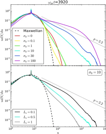
4.1. Total spectra and maximum energy

This rather complex shock structure leads to efficient nonther-mal particle acceleration. The upper panel in Fig. 6shows the total particle spectrum, udN/du, where u = γβ is the dimen-sionless particle momentum at time ωpet = 3920 for all the magnetizations simulated here. As expected, the unmagnetized shock produces a high-energy power-law tail extending beyond the thermal bath. For σ0= 0.1, particle acceleration is quenched in most of the shock front (thermal spectrum), except in the low-field regions which produces a weak excess starting below udN/du . 10−4 _{and extending to the same maximum energy} as in the unmagnetized shock. In contrast, strongly magnetized shocks (σ0 > 1) present a pronounced high-energy power-law tail extending to energies far beyond unmagnetized shocks, with a maximum Lorentz factor γmax/Γ0∼ 500 for σ0= 30 compared with γmax/Γ0 ∼ 20 for σ0 = 0. The power law hardens as well with increasing magnetization, approaching the canonical first-order Fermi acceleration spectrum dN/du ∝ u−2.2for σ0 = 30. At this magnetization, the spectrum breaks and steepens at high energy (γ & 300) and a new component emerges whose nature

Fig. 3.Top: plasma bulk momentum along the x-direction, Ux = ΓVx/c, for σ0 = 30 over the full simulation box at time ωpet= 3920. Bottom:

zoomed-in view of the equatorial region of the shock front shown by the rectangular box in the upper panel. Solid black lines with arrows are the plasma velocity streamlines.

will become clear later. The bottom panel in Fig. 6shows the dependence of the particle spectrum with the striped wind filling factor, Ls/Ly. Particle acceleration is more pronounced at low Ls, which is consistent with the trend reported earlier that parti-cle acceleration is more effective when the wind is more magne-tized on average; that is, ¯σ0 ≈ 4.5 for Ls/Ly= 0.1, as compared with ¯σ0≈ 0.65 for Ls/Ly= 1.

Figure 7 shows the time evolution of the maximum parti-cle Lorentz factor of the total spectrum, γmax(t). For the unmag-netized shock (σ0 = 0), the maximum energy approximately grows as γmax/Γ0 ≈ 0.5√ωpet without any sign of saturation, in agreement with Sironi et al.(2013). The square-root depen-dence reflects the microscopic nature of the Weibel-driven tur-bulence. Finite but mildly magnetized solutions (σ0 = 0.1, 1, 10) show a similar acceleration rate at the early stages, but this is followed by a saturation at ωpet & 500 which is particu-larly visible for the σ0 = 0.1 solution. This saturation is related to the finite size of the turbulent region in the upstream flow, which approximately scales as the particle Larmor radius in the background field (Lemoine & Pelletier 2010;Sironi et al. 2013;

Plotnikov et al. 2018).

For uniform shocks, there would be no more evolution of the particle spectrum. In contrast, we observe here that the maxi-mum energy then increases again and at a much faster rate in the late evolution of the simulation. For σ0= 1, γmaxincreases again at ωpet & 2 × 103. For σ0 = 10, it occurs earlier, at ωpet & 103, followed by a quasi-linear evolution γmax∝ t. More highly mag-netized solutions (σ0 = 30, 100) only show a linear evolution of the maximum particle energy with time from the beginning of the simulations. The longest runs (σ0 = 10 and 30) show no sign of saturation. The linear increase of the particle energy with time is evidence for efficient particle acceleration, compatible

400 200 0 200 400

y/d

V/

c

x/d

= 1500

V

/c

V

/c

Fig. 4.Plasma bulk velocity profile in the downstream flow along the x-and y-directions at x/de= 1500 for σ0= 30 at time ωpet= 3920.

with the Bohm regime but in sharp contrast with shock acceler-ation mediated by self-generated microturbulence (Sironi et al. 2013).

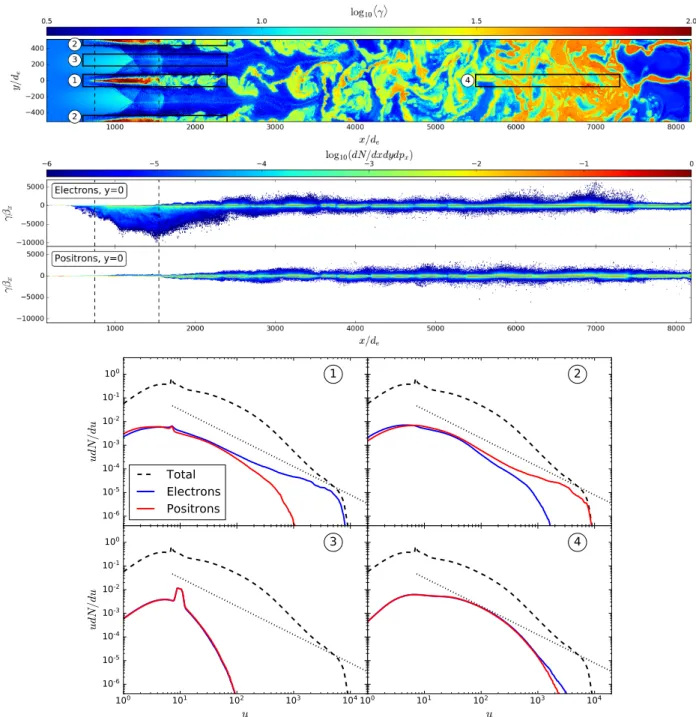
4.2. Phase space and local spectra

To gain further physical insight into the origin and location of par-ticle acceleration, we compute the mean parpar-ticle Lorentz factor, hγi, in each cell of the simulation as reported in the top panel in Fig.8 at ωpet = 7840. High-energy particles are located in

Fig. 5. Top: magnitude of the total electric current density, |J|, normalized by the fiducial upstream current J0 = cB0/4πLyfor σ0 = 30 at

ωpet= 7840. The white arrows schematically show how the current flows and closes within the simulation box. Bottom: plasma charge density, ρ,

normalized by the fiducial upstream charge density J0/c.

10-5 10-4 10-3 10-2 10-1 100

ud

N

/d

u

p

_{= 2}

.

2

ω

t

=3920

Maxwellian

σ

= 0

σ

= 0

.

1

σ

= 1

σ

= 10

σ

= 30

σ

= 100

u

ud

N

/d

u

p

_{= 2}

.

2

σ

= 10

L

= 0

.

1

L

= 0

.

5

L

= 1

Fig. 6.Top: total particle spectrum as a function of the dimensionless total particle momentum, u= γβ for all the magnetizations explored in this study and at the same time ωpet= 3920. Bottom: effect of the striped

wind filling factor on the final particle spectrum, Ls/Lyfor σ0 = 10 at

the same time as in the top panel. The black dotted line shows a power law dN/du ∝ u−p_{of index 2.2. The black dashed line is a 2D relativistic}

Maxwellian distribution for comparison.

high-density regions within the current layers and inside the spearhead-shaped cavities at the shock front. A look into the x–px phase-space distribution within the midplane reveals that the latter contain the highest energy particles in the simulations, γ ∼ 104_,

102 ₁₀3 ₁₀4

ω

t

γ

_t

t

Fig. 7.Time evolution of the maximum particle Lorentz factor of the total spectrum, γmax, in all the runs. The dashed black lines show γmax=

0.5Γ0√ωpetand γmax= 0.5Γ0ωpet.

in the form of a strongly beamed distribution traveling against the incoming flow. Electrons (positrons) are preferentially acceler-ated in the equatorial (polar) cavities and vice versa ifΩ · B < 0. The asymmetry between both species as well as the anisotropy of their momentum distribution decrease downstream and even fully disappear where the flow becomes turbulent (x/de& 4000). The bottom panels in Fig.8show the particle spectra measured in four areas defined in the top panel. Areas 1 and 2 are restricted to the shock-front cavities. The asymmetric acceleration between elec-trons and posielec-trons is clearly visible here. In contrast to the total spectrum, the spectrum measured in these cavities is consistent with a single power law extending from γmin= Γ0to γmax ≈ 104 with an index close to but slightly harder than −2.2. Area 3 is limited to the shock front at intermediate latitudes where particle acceleration is quenched. Area 4 focuses on the far-downstream region where the current layers reconnect and merge in a turbu-lent manner. The spectrum is hard at low energies, but cuts off

10-6 10-5 10-4 10-3 10-2 10-1 100

ud

N

/d

u

1

Total

Electrons

Positrons

2

u

ud

N

/d

u

3

u

4

Fig. 8.Top panel: mean particle Lorentz factor at ωpet= 7840 for σ0 = 30. Middle panels: electron and positron x–pxphase-space distribution

dN/dxdydpxalong the midplane integrated within y/de± 75. Bottom panels: local particle spectra measured at four locations shown in the top

paneland labeled from 1 to 4 . The dashed line is the total spectrum, and the dotted line is dN/du ∝ u−2.2_{for reference.}

noticeably below the maximum energy measured in the cavities. This difference explains the high-energy break at γ & 300 in the total spectrum, beyond which the spectral component from the shock-front cavities takes over.

4.3. Particle trajectories

Figure9shows two typical high-energy particle trajectories out of a randomly selected sample of 2000 particles for σ0 = 30, which are meant to illustrate the different acceleration processes at work. Particle 1 shown in the left panels represents the accel-eration history of the highest energy particles found in the simu-lations. As already pointed out in Sect.4.2, these particles inflate

the elongated cavities near the shock front and in the upstream medium. In the early phases (ωpet . 2500), the particle is trapped inside the cavity with little acceleration. At ωpet ∼2500, the shock front catches up with the particle, which leads to a rapid and uninterrupted acceleration up to at least γ & 2000. During this phase, the particle is trapped in a region that looks like a wake produced behind the cavities where the current layer forms and departs from. The particle trajectory moves back and forth across the equatorial plane where the magnetic field reverses, such that it is well described by the relativistic ana-log of Speiser orbits (Speiser 1965;Cerutti et al. 2012). As the particle surfs on the wake, its Larmor radius becomes su ffi-ciently large to experience the strong macroscopic bulk-velocity

Fig. 9.Typical high-energy particle trajectories accelerated at the shock front (left panels) and in the turbulent downstream medium (right panels) for σ0 = 30. Top panels: the Lorentz factor is color-coded along the particle trajectories, itself plotted on top of the plasma density map (gray

scale) at the final time of the particle tracking. Bottom panels: time evolution of the particle Lorentz factor.

shear, and therefore we associate the acceleration of these particles with the tangential shear-flow acceleration mechanism, which in essence is another form of the Fermi process. In this regime, the energy gain is due to Lorentz-frame transformation as the particle is scattered back and forth across the velocity-shear layer, and is of order∆γ/γ ∼ Γs− 1 after each crossing, whereΓs= 1/

p

1 −∆V2/c2_{, and}∆V = (V

1− V2)/(1 − V1V2/c2) is the velocity shear sampled by the particle between frames 1 and 2 (Ostrowski 1990; Rieger & Duffy 2004). In this simula-tion, the velocity shear is mildly relativistic,∆V/c ∼ 0.8, leading to∆γ/γ ∼ 0.7. The acceleration proceeds until the particle is kicked out and advected downstream, which plays the role of an escape mechanism.

Particle 2 is more representative of particles accelerated in the turbulent flow further downstream, and therefore of the bulk of the energetic particles in the simulations. It is injected at inter-mediate latitudes and flows in the laminar magnetized medium between the equatorial and polar current layers without signifi-cant energy gain. At ωpet ∼5000, the particle is captured by a current layer where it experiences an abrupt acceleration, from γ ∼ Γ0to γ ∼ 200. We associate this impulsive phenomenon as direct acceleration via relativistic reconnection occurring within the current sheet, which naturally boosts the particle energy to γ ∼ Γ0σ0 = 200 (e.g., Werner et al. 2016). This event is fol-lowed by a much slower stochastic acceleration. At this stage, the particle has reached the turbulent flow where current layers are mixed together and collide at nearly random velocities. This environment favors multiple particle scattering which leads to a stochastic increase or decrease of its energy, but with a net pos-itive gain. In this sense, this process is reminiscent of a second-order Fermi acceleration.

5. Synchrotron radiation

Figure10shows the instantaneous synchrotron spectrum emitted by the pairs in the σ0= 30 simulation at ωpet= 7840, assuming the plasma is optically thin everywhere. To reconstruct the

spec-10-2 ₁₀-1 ₁₀0 ₁₀1 ₁₀2 ₁₀3 ₁₀4 ₁₀5 ₁₀6 ₁₀7 ₁₀8 ₁₀9

ν/ν

a

b

c

Fig. 10.Total synchrotron spectrum for σ0 = 30 at ωpet= 7840 (blue

solid line). The dashed lines show the spectra emitted near the shock front (red) and in the far-downstream region (black). The dotted line

is a pure power law which would be emitted by a p = 2.2 power-law

electron spectrum, such that dE/dtdν ∝ ν(−p+1)/2_{= ν}−0.6_{. The frequency}

bands labeled a , b , and c refer to Fig.11.

trum, we use a delta-function approximation. Each particle emits a single photon radiating away the total power lost by the par-ent particle, Psync, with a frequency set by the synchrotron criti-cal frequency. We recriti-call here that radiative losses are neglected in the simulations for simplicity, and therefore the synchrotron spectrum computed here is not meant to be compared with, for instance, the observed Crab Nebula spectrum, which most likely results from a cooled particle distribution. Instead, our goal here is to characterize the main emission pattern at the shock in dif-ferent frequency bands. The power spectrum of a single photon is then given by dE dtdν ≈ Psyncδ (ν − νc), (12) where Psync = 2 3r 2 ecγ 2_B˜2 ⊥, (13)

Fig. 11.Spatial distribution of the synchrotron radiation flux integrated in the frequency bands defined in Fig.10: a (ν/ν0< 102), b (102< ν/ν0<

106_{), and c (ν/ν} 0> 106).

re= e2/mec2is the classical radius of the electron, and νc=

3e 4πmec

γ2_˜

B⊥, (14)

is the critical synchrotron frequency. ˜B⊥is the effective perpen-dicular (to the particle velocity vector) magnetic field in the pres-ence of a strong electric field given by (e.g.,Cerutti et al. 2016)

˜

B⊥= E + β × B − (β · E) β. (15)

Frequencies are normalized by the fiducial synchrotron critical frequency ν0= 3e 4πmec Γ2 0B0. (16)

The total synchrotron spectrum presents three main features: (i) a low-energy bump centered around ν/ν0 ∼ 1, (ii) a plateau at intermediate frequencies (dE/dtdν ∝ ν0_{, 10}1 _{. ν/ν}

0 . 104) followed by, (iii) a steep power-law decline cutting off at ν/ν0∼ 108_{. The latter is slightly steeper than the canonical dE/dtdν ∝} ν(−p+1)/2 _{= ν}−0.6 _{synchrotron spectrum emitted by a p = 2.2} power-law electron spectrum immersed into a uniform magnetic field.

The bulk of the synchrotron spectrum originates from the far-downstream region where the flow isotropizes and turbu-lent reconnection accelerates the particles (see black dashed line in Fig.10). The spectrum emitted in the vicinity of the shock front is composed of the low-energy bump and a hard power-law tail (dE/dtdν ∝ ν−0.3) spanning over nearly seven orders of magnitude in frequency range. The contribution from the shock front is subdominant at almost all frequencies except at the high-end of the spectrum, ν/ν0 & 106 where it rises above the steeper spectrum of the far-downstream region. Figure 11

shows the spatial distribution of the emitted synchrotron flux integrated in three frequency bands: (i) low-, ν/ν0 < 102, (ii) intermediate-, 102 _{< ν/ν}

0 < 106, and (iii) high-frequency band ν/ν0> 106labeled as a , b and c respectively. The low-energy flux is rather uniformly distributed in the downstream flow, that is, from the shock front to the back end of the numerical box,

from the most magnetized regions to the current layers, but with the notable exception of the shock front cavities. At intermedi-ate frequencies in band b , the emission in concentrated within the outer edges of the current layers up to the shock front cav-ities which are lighting up in this band. Although high-energy particles are also located inside the layers (see Fig.8), they do not emit significant radiation because the fields almost vanish in there. Away from the current layers, in smooth magnetized regions, the field is high but energetic particles are absent lead-ing to no flux from these regions. In the high-energy band ( c ), the emission is dominated by the edges of the shock-front cav-ities piercing through the upstream, as well as by the base of the current sheets in the near downstream medium. The rest of the upstream flow remains dark in all bands as expected because

˜ B⊥ ≈ 0.

6. Discussion and conclusion

Here, we show that the anisotropic nature of the pulsar wind has a dramatic effect on the structure and evolution of the shock front. The usual local plane-parallel approximation does not apply because of the critical role of the global dynamics of the down-stream flow, and therefore a latitudinally broad simulation box is essential. A salient feature is the formation of a sharp velocity shear between strongly- and weakly magnetized regions, which combined with current-driven instabilities leads to strong plasma turbulence in the downstream flow. Current sheets forming in the equatorial plane and at the poles mix and reconnect lead-ing to efficient nonthermal particle acceleration. The efficiency of particle acceleration increases with σ, which is similar to rel-ativistic reconnection but opposite to Fermi acceleration in uni-form shocks. Turbulent reconnection leads to a power-law elec-tron spectrum with a slope that hardens with σ, as expected from recent studies of relativistic reconnection (Sironi & Spitkovsky 2014;Werner et al. 2016) and kinetic turbulence (Zhdankin et al. 2017,2018). Scaled up to the Crab Nebula, with dN/dγ ∝ γ−2.2, the injected (uncooled) X-ray electron spectrum is consistent with the high-σ shock solution σ0 = 30, or a mean upstream magne-tization ¯σ0 ≈ 5. This result is compatible with global 3D MHD

models which advocate high-σ solutions to explain the morphol-ogy of the Crab Nebula (Porth et al. 2013,2014). The spectrum extends fromΓ0to ∼Γ0σ0beyond which it steepens significantly and where another component takes over and extends the total spectrum to even higher energies. It is tempting to connect this result with the mysterious high-energy break in the Crab Neb-ula spectrum, where the electron spectral index decreases by ∼0.5 (Meyer et al. 2010).

The high-energy component originates from another robust and extraordinary feature of anisotropic magnetized shocks, which is the formation of elongated cavities at the base of the polar and equatorial regions drilling through the upstream medium. These structures are low-field, low-density regions moving with mildly relativistic speeds against the incoming flow, and their sizes continuously grow with time. They are inflated by the highest energy particles in the box, which follow relativistic Speiser orbits. These special trajectories, typically found in reconnection layers, are captured by the midplane where the magnetic field polarity reverses. This trapping mecha-nism provides stability to the cavities themselves, whose sizes constantly adjust to the particle Larmor radius. These parti-cles are energized via shear-flow acceleration at the interface between the cavities and the incoming flow. This component alone explains the highest-energy part of the particle spectrum. The maximum particle energy increases nearly linearly with time, γmax ∝ t, in contrast to Weibel-dominated shock accel-eration where γmax ∝

√

t (Sironi et al. 2013; Plotnikov et al. 2018), meaning that the acceleration process is very efficient, close to the Bohm limit. Another important difference with Weibel-dominated shock acceleration is that the particle spec-trum does not show signs of saturation, the maximum energy grows steadily until the end of the simulations. Presumably, the particle energy will be limited by the transverse size of the shock or by radiative losses such as those in the Crab Nebula where the electron maximum energy is limited by the synchrotron burn-off limit (Guilbert et al. 1983; de Jager et al. 1996). These cavities also have the peculiarity to preferentially accelerate one sign of charge, electrons in the equatorial region, positrons (ions) at the poles, and vice versa ifΩ · B < 0, as also reported by

Giacinti & Kirk(2018).

The modeling of synchrotron radiation indicates that while the bulk of the emission is produced quasi-isotropically in the downstream region, the high-end of the synchrotron spectrum is concentrated within the edges and the wakes of the shock front cavities where both the field and the particle energy are the highest. Translated in terms of the Crab Nebula features, we predict that the 100 MeV emission is preferably localized at the inner ring, and specifically on the side receding away from us as the emission in the cavities is Doppler boosted in the direc-tion opposite to the incoming pulsar wind. There might also be a weaker contribution from the base of the counter jet because of the smaller volume involved in comparison with the equa-torial region. The wake behind the cavities is highly dynami-cal. Due to the kink instability, the high-energy beam sweeps a wide angular range. Therefore, gamma-ray flares at the high end of the synchrotron spectrum come out as a natural conse-quence of particle acceleration at the pulsar wind termination shock, and more generally in any relativistic, magnetized, and anisotropic shocks with a possible application to the hotspots of relativistic jets and gamma-ray bursts. The mildly relativistic bulk motion of the backflow, withΓ ∼ 3−4, would naturally push the radiation energy above the rest-frame 160 MeV synchrotron burn-off limit, a persistent feature of the Crab Nebula gamma-ray flares (Tavani et al. 2011;Abdo et al. 2011). Although these

results suggest a connection between particle acceleration in the cavities and gamma-ray flares, more work is needed for a solid conclusion.

An obvious limitation of the proposed model is its Carte-sian plane-parallel geometry. Any curvature of the shock front and the radial expansion of the downstream flow are therefore neglected in this work. A more realistic configuration with a spherical geometry and a finite curvature of the shock front would be the logical next step to confirm our findings. This would also break the symmetry between the poles and the equator, which play nearly identical roles in this study. In particular, the cav-ity in the equator may then have a dominant contribution in the acceleration (charge asymmetry) and radiation pattern (gamma-ray flares) because of its larger volume in comparison with the poles. An extension to 3D simulations would also be desirable to fully capture magnetic reconnection that occurs here in the out-of-plane direction and therefore some of the important features of reconnection are missing here (e.g., tearing mode and plasmoid formation). Three-dimensional simulations can also capture pos-sible departures from axisymmetry, which may explain for instance the knotty nature of the inner ring in the Crab Nebula. Synchrotron cooling could play an important role in the dynam-ics of the shock front cavities where it is most severe. Although they are probably highly subdominant in number compared with pairs, ions are most likely present in the wind and in the neb-ula. If the efficient particle acceleration mechanism revealed in this work also applies to them, pulsar wind nebulae could be an important source of the Galactic cosmic-ray population. Dissipa-tion of the oscillating current sheet in the pulsar wind may lead to efficient particle acceleration ahead of the termination shock (Cerutti & Philippov 2017). An excess of energetic particles in the equatorial regions may affect the shock dynamics in return. The exploration of all of the above effects provides a wide array of possible future investigations.

Acknowledgements. We are grateful to the anonymous referee for his/her very supportive report. This work has been supported by the Programme National des Hautes Énergies of CNRS/INSU and CNES. We acknowledge PRACE and GENCI (allocations A0050407669 and A0070407669) for awarding us access to Joliot-Curie at GENCI@CEA, France.

References

Abdo, A. A., Ackermann, M., Ajello, M., et al. 2011,Science, 331, 739

Achterberg, A., Gallant, Y. A., Kirk, J. G., & Guthmann, A. W. 2001,MNRAS, 328, 393

Amato, E. 2020, ArXiv e-prints [arXiv:2001.04442] Amato, E., & Arons, J. 2006,ApJ, 653, 325

Bednarz, J., & Ostrowski, M. 1998,Phys. Rev. Lett., 80, 3911

Begelman, M. C. 1998,ApJ, 493, 291

Begelman, M. C., & Kirk, J. G. 1990,ApJ, 353, 66

Bogovalov, S. V. 1999,A&A, 349, 1017

Cerutti, B., & Philippov, A. A. 2017,A&A, 607, A134

Cerutti, B., & Werner, G. 2019, Astrophysics Source Code Library [record ascl:1911.012]

Cerutti, B., Uzdensky, D. A., & Begelman, M. C. 2012,ApJ, 746, 148

Cerutti, B., Werner, G. R., Uzdensky, D. A., & Begelman, M. C. 2013,ApJ, 770, 147

Cerutti, B., Mortier, J., & Philippov, A. A. 2016,MNRAS, 463, L89

Coroniti, F. V. 1990,ApJ, 349, 538

de Jager, O. C., Harding, A. K., Michelson, P. F., et al. 1996,ApJ, 457, 253

Demidem, C., Lemoine, M., & Casse, F. 2018,MNRAS, 475, 2713

Gallant, Y. A., Hoshino, M., Langdon, A. B., Arons, J., & Max, C. E. 1992,ApJ, 391, 73

Giacinti, G., & Kirk, J. G. 2018,ApJ, 863, 18

Greenwood, A. D., Cartwright, K. L., Luginsland, J. W., & Baca, E. A. 2004,J. Comput. Phys., 201, 665

Hoshino, M., Arons, J., Gallant, Y. A., & Langdon, A. B. 1992,ApJ, 390, 454

Kennel, C. F., & Coroniti, F. V. 1984,ApJ, 283, 710

Keshet, U., Katz, B., Spitkovsky, A., & Waxman, E. 2009,ApJ, 693, L127

Kirk, J. G., Guthmann, A. W., Gallant, Y. A., & Achterberg, A. 2000,ApJ, 542, 235

Kirk, J. G., Lyubarsky, Y., & Petri, J. 2009, in The Theory of Pulsar Winds and Nebulae, ed. W. Becker,Astrophys. Space Sci. Lib., 357, 421

Komissarov, S. S. 2013,MNRAS, 428, 2459

Langdon, A. B., Arons, J., & Max, C. E. 1988,Phys. Rev. Lett., 61, 779

Lemoine, M. 2016,J. Plasma Phys., 82, 635820401

Lemoine, M., & Pelletier, G. 2010,MNRAS, 402, 321

Lemoine, M., Gremillet, L., Pelletier, G., & Vanthieghem, A. 2019,Phys. Rev. Lett., 123, 035101

Lyubarsky, Y. E. 2003,MNRAS, 345, 153

Medvedev, M. V., & Loeb, A. 1999,ApJ, 526, 697

Meyer, M., Horns, D., & Zechlin, H. S. 2010,A&A, 523, A2

Michel, F. C. 1973,ApJ, 180, L133

Olmi, B., Del Zanna, L., Amato, E., & Bucciantini, N. 2015,MNRAS, 449, 3149

Ostrowski, M. 1990,A&A, 238, 435

Pelletier, G., Bykov, A., Ellison, D., & Lemoine, M. 2017,Space Sci. Rev., 207, 319

Pétri, J., & Lyubarsky, Y. 2007,A&A, 473, 683

Plotnikov, I., Grassi, A., & Grech, M. 2018,MNRAS, 477, 5238

Porth, O., Komissarov, S. S., & Keppens, R. 2013,MNRAS, 431, L48

Porth, O., Komissarov, S. S., & Keppens, R. 2014,MNRAS, 438, 278

Rees, M. J., & Gunn, J. E. 1974,MNRAS, 167, 1

Rieger, F. M., & Duffy, P. 2004,ApJ, 617, 155

Sironi, L., & Spitkovsky, A. 2011,ApJ, 741, 39

Sironi, L., & Spitkovsky, A. 2014,ApJ, 783, L21

Sironi, L., Spitkovsky, A., & Arons, J. 2013,ApJ, 771, 54

Speiser, T. W. 1965,J. Geophys. Res., 70, 4219

Spitkovsky, A. 2008,ApJ, 682, L5

Tavani, M., Bulgarelli, A., Vittorini, V., et al. 2011,Science, 331, 736

Werner, G. R., Uzdensky, D. A., Cerutti, B., Nalewajko, K., & Begelman, M. C. 2016,ApJ, 816, L8

Zhdankin, V., Werner, G. R., Uzdensky, D. A., & Begelman, M. C. 2017,Phys. Rev. Lett., 118, 055103

Zhdankin, V., Uzdensky, D. A., Werner, G. R., & Begelman, M. C. 2018,ApJ, 867, L18