HAL Id: hal-00003157
https://hal.archives-ouvertes.fr/hal-00003157
Submitted on 24 Oct 2004
HAL is a multi-disciplinary open access
archive for the deposit and dissemination of sci-entific research documents, whether they are pub-lished or not. The documents may come from teaching and research institutions in France or abroad, or from public or private research centers.
L’archive ouverte pluridisciplinaire HAL, est destinée au dépôt et à la diffusion de documents scientifiques de niveau recherche, publiés ou non, émanant des établissements d’enseignement et de recherche français ou étrangers, des laboratoires publics ou privés.
heterogeneous and rough substrates
Joël de Coninck, Salvador Miracle-Solé, Jean Ruiz
To cite this version:
Joël de Coninck, Salvador Miracle-Solé, Jean Ruiz. Rigorous generalization of Young’s law for hetero-geneous and rough substrates. Journal of Statistical Physics, Springer Verlag, 2003, 111, pp.107-127. �hal-00003157�
heterogeneous and rough substrates
J. De Coninck,
1S. Miracle–Sol´
e,
2and J. Ruiz
3Abstract: We consider a SOS type model of interfaces on a substrate which is both heterogeneous and rough. We first show that, for appropriate values of the parameters, the differential wall tension that governs wetting on such a substrate satisfies a generalized law which combines both Cassie and Wenzel laws. Then in the case of an homogeneous substrate, we show that this differential wall tension satisfies either the Wenzel’s law or the Cassie’s law, according to the values of the parameters.
Key words: SOS models, Wenzel’s law, Cassie’s law, wetting, roughness, interfaces.
1
Introduction
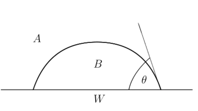
The wettability of surfaces plays an important role in many technological processes. Since Young’s work, two centuries ago, one usually characterizes the wetting properties of a surface by measuring the associated contact angle (see Fig. 1) of a reference sessile drop, of a liquid B on the surface W (also
Preprint CPT–2002/P.4381, published in J. Stat. Phys. 111, 107–127 (2003)
1
Centre de Recherche en Mod´elisation Mol´eculaire, Universit´e de Mons–Hainaut, 20 place du Parc, B-7000 Mons, Belgium.
E-mail address: Joel.De.Coninck@galileo.umh.ac.be
2
Institut des Hautes Etudes Scientifiques, F-91440, Bures-sur-Yvette, France. Perma-nent address: Centre de Physique Th´eorique, CNRS, Luminy case 907, F-13288 Marseille Cedex 9, France.
E-mail address: Salvador.Miracle-Sole@cpt.univ-mrs.fr
3
Centre de Recherche en Mod´elisation Mol´eculaire, Universit´e de Mons–Hainaut, 20 place du Parc, B-7000 Mons, Belgium. Permanent address: Centre de Physique Th´eorique, CNRS, Luminy case 907, F-13288 Marseille Cedex 9, France.
called substrate or wall) in equilibrium inside a medium A, leading to the classical Young’s equation
τABcos θ = τAW − τBW (1.1) ❇ ❇ ❇ ❇ ❇ ❇ ❇❇ θ A B W
Fig. 1: Young’s contact angle
where τij refers to the interfacial tension between the two media i and j and
θ is the equilibrium contact angle of the droplet on the substrate W . It is assumed here that τAB is isotropic (an irrelevant hypothesis in the present
study which concerns the right hand side of equation (1.1)).
In the general case of an orientation dependent surface tension for the AB–interface, the equilibrium shape of the sessile drop is determined by the Winterbottom’s construction [W]. As a consequence of this construction the contact angle θ satisfies, in dimension d = 1, the modified Young’s equation:
cos θ τAB(n) − sin θ
∂
∂θτAB(n) = τAW − τBW (1.2) where n = (− sin θ, cos θ). This equation as well as the validity of Winter-bottom’s construction has been proved from microscopic arguments, within the 1-dimensional Solid-On-Solid models in [DD] [DDR] [MR]. For a truly microscopic model, the 2-d Ising model (rather than a coarsed-grained one like the SOS) a first proof of the modified equation (1.2) was given in [AK]. For this model the validity of Winterbottom’s construction was shown in [PV]. More recent proofs which hold in any dimensions are given in [BIV] [DGI] (see also references therein).
Equation (1.2) holds for flat and homogeneous surfaces. However, in practice a real surface is all except flat and homogeneous. It is therefore important to generalize this equation to take into account the real surfaces. It is known experimentally that whenever the surface is chemically het-erogeneous, say containing two species 1 and 2, a possible good equation is the Cassie’s law [C] given by
where c (resp. 1 − c) denotes the surface concentration of the specie 1 (resp. 2). This leads to
cos θ12= c cos θ1+ (1 − c) cos θ2 (1.4)
whenever the equilibrium contact angles θ1, θ2, and θ12 can be obtained.
For rough substrates, one often uses the Wenzel’s law [W]
cos θ|r = r cos θ|1 (1.5)
where r refers to the roughness of the surface defined as the ratio of the area A of the surface and the area ¯A of its projection on the horizontal plane.
In the present paper, we consider a SOS model and we extend these results obtaining a generalized equation. It reduces to Cassie’s equation whenever the substrate is flat but heterogeneous and to Wenzel’s equation whenever the substrate is homogeneous but rough.
Let us stress that we assume within this approach that we are dealing with equilibrium contact angles. The case of dynamics will be developed elsewhere.
The paper is organized as follows. The model is introduced in Section 2. The generalized Young’s relation for rough and heterogeneous substrates is given in section 3. In section 4, we consider a particular geometry of an homogeneous wall and show that there is a transition between a Wenzel’s regime and a Cassie’s regime. The proofs of the results are given in the appendix.
2
The model
To describe the A|B interface between liquid and air for instance, we consider a SOS type model on a d–dimensional lattice, d = 1, 2, defined as follows. At each site i of a finite box Λ ⊂ Zd, we assign an integer variable h
i which
represents the height of the interface at this site. To a configuration h = {hi}i∈Λ, we associate its graph to be denoted Γ. Its area (or length) is
|Γ| = |Λ| +P
hi,ji⊂Λ|hi− hj|, where the sums runs over all pairs of nearest
neighbours of Λ.
We want here to study this interface on top of a substrate which is both heterogeneous and rough. The substrate is thus represented by another SOS interface W , union of two disjoint subsets W1 and W2, with disjoint
projec-tions Λ1 ⊂ Λ and Λ2 = Λ\Λ1, and respective height configurations {h(1)i }i∈Λ1,
and {h(2)i }i∈Λ2. We let ¯hi = h
(1)
i when i ∈ Λ1 and ¯hi = h (2)
i when i ∈ Λ2.
This wall W as well as W1, W2, Λ1, and Λ2 are assumed to be periodic
with periodicity a = (a1, ..., ad) ∈ (Z+)d, that is h(1)i = h (1) i+a and h (2) i = h (2) i+a.
The respective roughness r1 and r2 read rk = |Wk| |Λk| = 1 + P hi,ji⊂Λk|h (k) i − h (k) j | |Λk| , k = 1, 2
The energy of the system is defined by
HΛ(Γ, W ) = JAB|Γ \ (Γ ∩ W )| + JAW1|Γ ∩ W1| + JAW2|Γ ∩ W2|
+ JBW1|W1\ (Γ ∩ W1)| + JBW2|W2\ (Γ ∩ W2)| (2.1)
Here Γ is above W , which means hi ≥ ¯hi for all i. and k = 1 or 2. The
set Γ \ (Γ ∩ W ) is relative to the AB microscopic interface, Γ ∩ W1 (resp.
Γ ∩ W2) is relative to the contact zone between A and W1 (resp. W2), and
W1\ (Γ ∩ W1) (resp. W1\ (Γ ∩ W2)) is relative to the contact zone between
B and W1 (resp. W2).
This system describes a system of droplets of a phase B inside a medium A on top of the wall W . JAB, JAW1, JAW2, JBW1, and JBW2 are the energies
per unit area of the corresponding microscopic interfaces (see Fig. 2).
••••••••••••• ••⋄⋄⋄⋄⋄⋄ ⋄⋄ ⋄•••••••••••••• ••⋄⋄⋄⋄⋄⋄⋄⋄⋄⋄••••••••⋄⋄ ⋄⋄⋄⋄⋄⋄⋄⋄⋄⋄⋄⋄⋄⋄⋄⋄⋄ ⋄•••••• A B Γ JAW1 JAW2 JAB JBW1 JBW2 W1 W2
Fig. 2: A configuration of the interface Γ on the substrate W = W1∪ W2.
Let us introduce the different free energies associated to the correspond-ing macroscopic interfaces. To define the free energy associated to the AB interface corresponding to a given slope n (a unit vector of Rd+1), we
intro-duce the Gibbs ensemble G(n, Λ) which consists of all configurations with the boundary condition
where [n · i] denotes the integer part of the scalar product n · i, and the boundary ∂Λ is the set of sites of Λ that have a nearest neighbour in Zd\ Λ.
We will take Λ to be the parallelepipedic box Λ = {i ∈ Zd : |i
k| ≤ N ak, k =
1, . . . , d}.
The surface tensions τAB and τAW are defined by the following
thermo-dynamic limits τAB(n) = lim N→∞− 1 βSn(Λ) log X Γ∈G(n,Λ) exp [−βJAB|Γ|] (2.2)
where Sn(Λ) is the area of the part of the hyperplane orthogonal to n passing
through the origin and included in the infinite cylinder of Rd+1 with basis Λ
and, τAW = lim N→∞− 1 β|Λ| log X∗ exp[−βHΛ(Γ, W )] (2.3)
where the sum P∗
runs over all configurations such that hi = ¯hi for all
i ∈ ∂Λ. Finally,
τBW = lim N→∞
JBW1|W1| + JBW2|W2|
|Λ| = r1c1JBW1 + r2c2JBW2 (2.4)
where c1 = |Λ1|/|Λ| and c2 = (1 − c1) = |Λ2|/|Λ| are the respective
concen-trations of W1 and W2.
That the limits exist follows from known arguments, see e.g. [DD, MMR]. In dimension one, the proof of (1.2) as well as the proof of the Winterbot-tom’s construction for the model under consideration may be obtained by an appropriate extension of the theory developed in [DDR] [MR] in the case of a flat and homogeneous substrate.
3
The generalized Young’s relation
Consider a drop of a phase B on top of the substrate W in a medium A. Three cases may appear: first, either the liquid B is always in contact with W or, second, there may be droplets of A between the liquid and W , or, finally, the medium A has no contact with the wall. Within our SOS model, these situations mean, first, that the ground state of the Hamiltonian of the system is given by the microscopic interface Γ that coincides with the substrate W , second, that the ground state microscopic interface Γ leaves holes between Γ and W , and, third, that the ground state microscopic interface Γ has no contact with the wall.
In this section we develop the first case and generalize to heterogeneous substrates Theorem 3.1 of [DMR], on the validity of Wenzel’s law for a rough but homogeneous substrate. We obtain a combination of both, Cassie’s and Wenzel’s laws.
To this end, we introduce the energy difference
HΛ′(Γ | W ) = HΛ(Γ, W ) − HΛ(W, W ) (3.1)
Since HΛ(W, W ) = JAW1|W1| + JAW2|W2| = (r1c1JAW1 + r2c2JAW2)|Λ| the
differential wall tension ∆τ ≡ τAW − τBW reads
∆τ = r1c1(JAW1− JBW1) + r2c2(JAW2 − JBW2) + lim N→∞− 1 β|Λ|log ZΛ (3.2) where ZΛ = X Γ e−βHΛ′(Γ|W ) (3.3)
Our first step is to write ZΛ as the partition function of a gas of elementary
excitations, simply also called excitations, which can be viewed as micro-scopic droplets over the substrate. These excitations are defined as follows. Given Γ and W , we consider the symmetric difference
∆ = (Γ ∪ W ) \ (Γ ∩ W ) (3.4)
We decompose ∆ into its maximal connected components δi, called
excita-tions, ∆ = δ1 ∪ δ2 ∪ · · · ∪ δn. Here, two components are said connected if
they are connected considered as subsets of Rd+1. A set {δ
1, δ2, . . . , δn} of
mutually disjoint excitations is called an admissible family of excitations. Then there exists a microscopic interface (SOS configuration) Γ, such that ∆ = δ1∪ δ2∪ · · · ∪ δn satisfies (3.4), namely
Γ = (∆ ∪ W ) \ (∆ ∩ W ) (3.5)
This correspondence between the admissible families of excitations and in-terface SOS configurations is one-to-one.
The energy difference H′
Λ reads in terms of families of excitations as
HΛ′(Γ | W ) = E(δ1) + · · · + E(δn) (3.6)
where
Indeed from the definitions (2.1) (3.1) we have
HΛ′ = JAB|Γ \ (Γ ∩ W )| − (JAW1 − JBW1)|W \ (Γ ∩ W1)|
− (JAW2 − JBW2)|W \ (Γ ∩ W2)|
which together with |Γ \ (Γ ∩ W )| = |∆ \ (∆ ∩ W )|, |W \ (Γ ∩ W1)| = |∆ ∩ W1|
and |W \ (Γ ∩ W2)| = |∆ ∩ W2| gives the expression (3.7) of the energy of
excitations. Then ZΛ = X ∆={δ1,...,δn} n Y i=1 e−βE(δi) (3.8)
where the sum runs over admissible families of excitations included in the infinite cylinder ΩΛ with basis Λ, ΩΛ = {(x1, . . . , xd+1) ∈ Rd+1 : |xk| ≤
N ak, k = 1, . . . , d}, and the product is taken equal to 1 if ∆ = ∅.
In the concept of excitation that we are considering, the configuration Γ = W , in which the microscopic interface is following the wall, is the ground state of the system. In other words, we assume that H′
Λ(Γ | W ) > 0 for all
Γ and N , or equivalently, that min
δ E(δ) > 0 (3.9)
In fact it is enough that this condition is satisfied for all excitations belonging to the set Ω(a) = {(x1, . . . , xd+1) ∈ Rd+1 : 0 ≤ xk ≤ ak, k = 1, . . . , d}.
We next consider arbitrary families of elementary excitations non neces-sarily mutually compatible and in which a given excitation can appear several times. To any such family {δ1, . . . , δn} a graph G(δ1, . . . , δn) is associated in
such a way that to each excitation corresponds (in a one-to-one way) a vertex of the graph, and there is an edge joining the vertices corresponding to δi
and δj whenever δi and δj are not compatible or coincide. We introduce the
clusters C as the non-empty arbitrary families of excitations for which the associated graph G(δ1, . . . , δn) is connected (this means that the excitations
draw a connected set in R2). Then we get
log ZΛ =
X
C
ΦT(C) (3.10)
where the sum runs over all clusters whose excitations belong to the infinite cylinder with basis Λ. The truncated functionals ΦT are defined by
ΦT(δ 1, . . . , δn) = a(δ1, . . . , δn) n! n Y i=1 e−βE(δi) (3.11) a(δ1, . . . , δn) = X G⊂G(δ1,...,δn) (−1)ℓ(G) (3.12)
Here the sum runs over all connected subgraphs G of G(δ1, . . . , δn), whose
vertices coincide with the vertices of G(δ1, . . . , δn), and ℓ(G) is the number
of edges of the graph G. If the cluster C contains only one excitation then a(δ) = 1.
To express condition (3.9) in terms of the coupling constants, we need a description of the substrate. Let Γz be the horizontal line at height z, that
is hi = z for all i. For any integer z such that infi¯hi + 1 ≤ z ≤ supi¯hi,
the difference W \ Γz splits into components that lies either below or above
Γz. They are called wells in the first case and we denote them by wk(z),
and protrusions in the second case (see Fig. 3). We let w0
k(z) denote the
projection of wk(z) on Γz and δk(z) = w0k(z) ∪ wk(z). We define
α1 = max z,k |δk(z) ∩ W1| |δk(z)| , α2 = max z,k |δk(z) ∩ W2| |δk(z)| (3.13) W Γz w1 w2 w01 w20 δ1 δ2
Fig. 3: The wells wk, their projections, w0k and the associated excitations δk(z).
Then condition (3.9) reads
C ≡ JAB − α1(JAB+ JAW1 − JBW1) − α2(JAB + JAW2 − JBW2) > 0 (3.14)
Let W denote the infinite periodic wall whose restriction to ΩΛ is given
by the previous height {h(1)i }i∈Λ1, {h
(2)
i }i∈Λ2, let Wa denote its restriction to
Theorem 1 Assume that the condition (3.14) is satisfied, then, for any βC > log νd+ 0.74, the following series, defining the differential wall
ten-sion, is absolutely convergent
∆τ = r1c1(JAW1− JBW1) + r2c2(JAW2 − JBW2) − 1 βa1· · · ad X b∈Wa X C∋b ΦT(C) |C ∩ W | (3.15)
The proof of the theorem is postponed to the appendix. It establishes a generalized law for rough and heterogeneous substrates:
∆τ = r1c1(∆τ )∗1+ r2c2(∆τ )∗2+ O(e−βC) (3.16)
where (∆τ )∗
1 and (∆τ )∗2 correspond to the case of a flat wall of the species 1
and 2 respectively.
A consequence of this result is that in the case of a rough and heteroge-neous wall both, the Wenzel’s and the Cassie’s laws, apply. These laws are satisfied up to a small temperature dependent correction (tending exponen-tially to zero with the temperature).
Referring to isotropic surfaces, one gets in terms of contact angles
cos θ = r1c1cos θflat1 + r2c2cos θ2flat+ O(e−βC) (3.17)
proving from microscopic argument the validity of eq. (9.3) in [SL].
The conditions for the validity of Theorem 1 are twofold. The restriction to low temperatures is of a technical nature and stems from the conditions needed to ensure the convergence of the used low temperature expansions. The condition (3.14) on the coupling parameters ensures that the ground state of the system coincides with the wall. Let us mention the study on Cassie’s law proposed in [DT] whose results do not rely on the knowledge of ground states. This condition is intimately related to the physics of the problem, and one may ask what happens whence increasing JAW1−JBW1 and
JAW2 − JBW2. This is the subject of the next section.
4
Transition between Cassie’s and Wenzel’s
regime
We will restrict our analysis to the case of an homogeneous substrate. Name-ly, we assume W2 = ∅, JAW1 = JAW, JBW1 = JBW, and JAW2 = JBW2 = 0.
periodicity be a in all directions. In dimension d = 2, we choose for any i ∈ {(i1, i2) ∈ Z2 : 0 ≤ i1 ≤ a − 1, 0 ≤ i2 ≤ a − 1}, ¯hi = ( −b for 0 ≤ i1 ≤ c − 1, and 0 ≤ i2 ≤ c − 1 0 otherwise (4.1)
The other heights are given by the periodicity: ¯h(i1+na,i2+na) = ¯h(i1,i2) see
Fig. 4. In dimension d = 1, we choose ¯hi = −b if 0 ≤ i ≤ c − 1, ¯hi = 0 if
c ≤ i ≤ a − 1, the periodicity giving the other heights : ¯hi+na = ¯hi.
a − c c b ◭c ◮◭ a − c ◮ N b H ¡¡ ¡¡ ¡¡ ¡¡ ¡¡ ¡¡ ¡ ¡¡ ¡¡ ¡¡ ¡¡ ¡¡ ¡¡ ¡¡ ¡¡
Fig. 4: The substrate surface W in dimensions 1 and 2.
4.1
Ground states
We define the specific energy per unit length as h(Γ, W ) = limN→∞ H(Γ,W )|Λ| .
We use Γkto denote the horizontal interface at height k i.e. such that hi = k
for all i. Notice that,
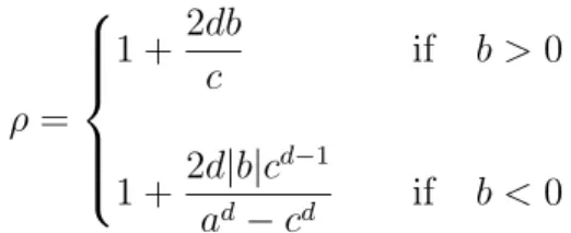
∆h(W ) ≡ h(W, W ) − rJBW = r(JAW − JBW) , (4.2) ∆h(Γ0) ≡ h(Γ0, W ) − rJBW = c′JAB + (1 − c′)(JAW − JBW) , (4.3) ∆h(Γk) ≡ h(Γk, W ) − rJBW = JAB, 1 ≤ k < +∞ . (4.4) where, c′ = ( (c/a)d if b > 0 1 − (c/a)d if b < 0 (4.5)
We let ρ = 1 + 2db c if b > 0 1 + 2d|b|c d−1 ad− cd if b < 0 (4.6)
From these formula, we get the following diagram of ground states (see Fig. 5). If JAW−JBW < ρ−1JAB the ground state is the wall W . If ρ−1JAB <
JAW − JBW) < JAB the ground state is Γ0. For JAW − JBW > JAB the Γk
are the ground states for any finite k ≥ 1.
◮ JAB NJAW − JBW ✏✏✏✏ ✏✏✏✏ ✏✏✏✏ JAW − JBW = JAB JAW − JBW = 1ρJAB W Γ0 Γk
Fig. 5: The diagram of ground states.
4.2
Wenzel’s regime
We will now consider the low temperature expansion of ∆τ when the ground state is W . The analysis of Section 3 applies directly to that case. The energy of excitations which are defined as in the previous section are given by Ew(δ) = JAB|δ \ (δ ∩ W )| − (JAW − JBW)|δ ∩ W | (4.7) By letting Cw = JAB− ρ(JAW − JBW) 1 + ρ we have Ew(δ) ≥ Cw|δ| (4.8)
Corollary 2 Assume that JAB−ρ(JAW−JBW) > 0, then for βCw > log νd+
0.74, the following series, defining the differential wall surface tension, is absolutely convergent ∆τ = r(JAW − JBW) − 1 βad X b∈Wa X C∋b ΦT(C) |C ∩ W | (4.9)
In this case Wenzel’s law applies in a first approximation.
4.3
Cassie’s regime
We will now consider the low temperature expansion of ∆τ when the ground state is Γ0.
For that we introduce the energy difference
HΛ′(Γ | Γ0) = HΛ(Γ, W ) − HΛ(Γ0, W ) (4.10)
We have
HΛ′(Γ | Γ0) = JAB|Γ \ Γ0| − [JAB− (JAW− JBW)](|Γ ∩ W | − |Γ0∩ W |) (4.11)
and the differential wall tension reads
∆τ = c′JAB + (1 − c′)(JAW − JBW) + lim N→∞− 1 β|Λ|log Z 0 Λ (4.12) where ZΛ0 =X Γ e−βHΛ′(Γ|Γ0) (4.13)
We now define the excitations as follows. Given Γ and Γ0, we consider the
symmetric difference
∆ = (Γ ∪ Γ0) \ (Γ ∩ Γ0) (4.14)
As in the previous section, we decompose ∆ in maximal connected compo-nents ∆ = δ1 ∪ δ2 ∪ · · · ∪ δn. The energy difference HΛ′ reads in terms of
families of excitations as H′
Λ(Γ | Γ0) = E0(δ1) + · · · + E0(δn) where
E0(δ) = Jℓv(δ) + [JAB− (JAW − JBW)](|δ ∩ Wu| − |δ ∩ Wd|) (4.15)
Here ℓv(δ) denotes the length of the vertical cells (bonds in dimension 1, or
plaquettes in dimension 2) of δ, Wu = W ∩ Γ0, and Wd= W \ Wu. Then,
ZΛ0 = X ∆={δ1,...,δn} n Y i=1 e−βE0(δi) (4.16)
and log ZΛ =PCΦ T
0(C) where the truncated functionals ΦT0 are defined by
(3.11) as before, but with E replaced by E0.
We let C0 = min ½ JAW − JBW 1 + c/d , JAB− (JAW − JBW) 2(cd+ 1) , ρ(JAW − JBW) − JAB 2ρ ¾ if b > 0 and C0 = min ½ JAB − (JAW − JBW) 4(a2− c2) , (JAW − JBW) − JAB/ρ 2c + a2 − c2 ¾ if b < 0 and d = 2.
Theorem 3 Assume that (1/ρ)JAB < JAW− JBW < JAB. Then, for βC0 >
log νd + 0.74, the following series, defining the differential wall tension, is
absolutely convergent ∆τ = c′JAB + (1 − c′)(JAW − JBW) − 1 βad X b∈Wa X C∋b ΦT 0(C) |C ∩ W | (4.17)
The proof is given in the appendix.
The corollary 2 and theorem 3 give the following transition between the Wenzel’s and Cassie’s regime:
i) If JAW − JBW < JAB/ρ, then
∆τ = r(∆τ )∗+ O(e−βCw
) (4.18)
which corresponds the Wenzel’s law
ii) If JAB/ρ < JAW − JBW < JAB, then
∆τ = c′τAB+ (1 − c′)(∆τ )∗+ O(e−βC0) (4.19)
which corresponds the Cassie’s law
4.4
the intermediate regime
Let us mention that when
JAW − JBW =
1 ρJAB
a degeneracy of ground states appears, their number tending to infinity in the thermodynamic limit. Indeed, with b > 0, any configuration following, at each pore, either the wall ∂W or the horizontal plane Γ0, is a ground
state with specific energy given by (4.2) or (4.3) (both expressions coincide in this case). This leads to the existence of a specific residual entropy at zero temperature S ≡ lim β→∞N→∞lim 1 |Λ|log ZΛ= 1 adlog 2
This might suggest that ∆τ behaves like ∆h − S/β around the point JAW −
JBW = 1ρJAB. We are planning to examine in a next work the possibility of
such kind of corrections at low temperature.
Remark 4 The discussion of the previous subsections extends to more gen-eral geometries of the wall. One can consider for example a wall composed of different rectangular wells with sizes given by (bk, ck). The phase diagram
of ground states will then exhibit different transition lines given by the corre-sponding ρ’s. Whence increasing the parameter JAW−JBW, the ground states
will move from the wall W to successive grounds states that fill different wells up to Γ0.
Acknowledgements
J.R. wishes to thank the Centre de Recherche en Mod´elisation Mol´eculaire– Universit´e de Mons–Hainaut for the enthusiasming atmosphere and the fi-nancial support during his stay. S. M. S. wishes to thank the Institut des Hautes ´Etudes Scientifiques, Bures-sur-Yvette (France), for the kind hospi-tality extended to him during the completion of this work.
Appendix
Proof of Theorem 1
The first ingredient is the following lower bound on the energy:
This bound follows from definitions (3.7) (3.13) by taking into account some easy geometrical observations.
The bound (A.1) ensures the convergence of the series P
δ∋xe−βE(δ) as
soon as βC > log νd, since the number of polygons (or of excitations δ) of
size ℓ passing to a given point is less then νℓ d .
Moreover using this bound, the proof of formula (3.15) as well as that of the absolute convergence of the series can be established following [GMM] (Chapter 4) in which the low temperature contours of the Ising model were considered in the role played here by the excitations. Indeed, the convergence of the cluster expansion holds, c.f. [D] [M], as soon as one can find a positive real-valued function µ(δ) such that
e−βE(δ)µ(δ)−1exp ½ X δ′ι δ µ(δ′) ¾ < 1 (A.2)
where the sum runs over excitations δ′ incompatible with δ: this relation is
denoted by δ′ι δ and means that δ′ do not intersect δ. Taking into account the
above remark on the entropy of excitations, that the lengths of excitations are even with minimal value |δmin| = 4, that Pδ′ιδµ(δ′) ≤ |δ|
P
δ′∋bµ(δ′),
and choosing µ(δ) = (νdet)−|δ|, inequality (A.2) will be satisfied whenever
βC > log νd+ t +
e−4t
1 − e−2t
The value t0 ≃ .61 that minimizes the function t + [e−4t/(1 − e−2t)] provides
the value 0.74 given in the theorem. The expression (4.9) then follows from (3.2) and (3.10) by letting N → ∞, taking into account that log ZΛ equals
X b∈W X C∋b ΦT(C) |C ∩ W |
up to a term that will disappear in the thermodynamic limit.
Proof of Theorem 3
The first step is to prove the following lower bound on the energy:
E0(δ) ≥ C0|δ| (A.3)
1–dimensional case
We partition δ in two disjoint subsets δ+ and δ− as follows. A vertical bond
belongs to δ+(respectively δ−) if it is above Γ
0(respectively below Γ0). Next,
consider the vertical line x = i + 1/2, i ∈ Z. These lines intersect δ in two points, one at height 0 and the other at positive or negative height. In the first case we let the two intersected bonds belong to δ+ and in the second
case we let them belong to δ−. Then δ+ as well as δ− splits into maximal
connected components: δ+= δ+
1 ∪ δ+2 ∪ · · · ∪ δn+, δ− = δ1−∪ δ2−∪ · · · ∪ δm−, and
the energy reads
E0(δ) = n X k=0 E0(δk+) + m X k=0 E0(δk−) (A.4)
By eq. (4.15), the energy of the components δ+ and δ− reads
E0(δk+) = Jℓv(δk+) + (J − K)|δk+∩ Wu| E0(δk−) = Jℓv(δ − k) − (J − K)|δ − k ∩ Wd| (A.5)
where hereafter J = JAB, K = JAW−JBW. We will drop below the subscript
k to δ±k but still thinking of it as a component of δ±.
Using ℓh(δ−) to denote the number of horizontal bonds of δ−, it is easy
to realize that E0(δ−) ≥ Kℓv(δ−) if δ−∩ Γ−b = ∅ Kℓv(δ−) − (J − K) ℓh(δ−) 2 if δ −∩ Γ −b 6= ∅ (A.6)
by taking into account that J ≥ K and that the number of horizontal bonds of δ−∩ W
d does not exceed ℓh(δ−)/2.
When δ−∩ Γ
−b = ∅, the two obvious bounds ℓh(δ−) ≤ 2c and ℓv(δ−) ≥ 2,
leads immediately to the inequality (c + 1)ℓv(δ−) ≥ ℓh(δ−) + ℓv(δ−) = |δ−| so
that
E0(δ−) ≥
K c + 1|δ
−| (A.7)
Coming to the case δ−∩ Γ
ℓv(δ−) ≥ 2b. Then E0(δ−) ≥ K · ℓv(δ−) + ℓh(δ−) 2 ¸ − Jℓh(δ −) 2 ≥ · ℓv(δ−) + ℓh(δ−) 2 ¸Ã K − J max ℓh(δ−) 2 ℓv(δ−) + ℓh(δ−) 2 ! ≥ · ℓv(δ−) + ℓh(δ−) 2 ¸Ã K − J max ℓh(δ−) 2 2b + ℓh(δ −) 2 !
The maximum is obtained whenever ℓh(δ−) reaches its maximum value, i.e.
for ℓh(δ−) = 2c. Thus, we get in that case
E0(δ−) ≥ (K − J/ρ)
|δ−|
2 (A.8)
Let us now turn to E0(δ+). When δ+∩ Wu = ∅, with the help of
inequal-ities ℓh(δ+) ≤ 2c and ℓv(δ+) ≥ 2, we argue as above for the proof of (A.7),
to get
E0(δ+) ≥
J c + 1|δ
+| (A.9)
Coming to the case δ+∩ W
u 6= ∅, it suffices to realize that |δ+∩ Wu| ≥ 1 2(c+1)ℓh(δ +) to get E0(δ+) ≥ Jℓv(δ+) + J − K 2(c + 1)ℓh(δ +) ≥ J − K 2(c + 1)|δ +| (A.10)
Then, the bound (A.3) follows, in dimension 1 for b > 0, from inequalities (A.7–A.10). The situation b < 0 is obviously identical inverting the role of c and a − c, and thus we will not deal with it. We now turn to the proof in the
2–dimensional case
As in the 1–dimensional case, we partition δ in two disjoint subsets δ+ and
δ−. A vertical plaquette belongs to δ+ (respectively δ−) if it is above Γ 0
(respectively below Γ0). Next we consider the vertical line x = i + (1/2, 1/2),
i ∈ Z2. These lines intersect δ in two points, one at height 0 and the other
at positive or negative height. We let the two intersected plaquettes belong to δ+ in the first case and to δ− in the second case. Then again, the energy
is given by (A.4-A.5). We split the rest of the proof of (A.3) in two part dealing first with
The case b > 0 Using ℓ∗
h(δ−) = ℓh(δ−∩ Γ−b) to denote the number of
horizontal plaquettes of δ−∩ Γ
−b, we notice that E0(δ−) satisfies the lower
bounds E0(δ−) ≥ ( Kℓv(δ−) if δ−∩ Γ−b = ∅ Kℓv(δ−) − (J − K)[ℓv(δ−) + ℓ∗h(δ−)] if δ−∩ Γ−b 6= ∅ (A.11) When δ−∩Γ
−b = ∅, the isoperimetric inequality yields ℓv(δ−) ≥ 4pℓh(δ−)/2.
Since ℓh(δ−) ≤ 2c2 we get ℓv(δ−) ≥ (2/c)ℓh(δ−) so that
E0(δ−) ≥
K 1 + c
2
|δ−| (A.12)
Coming to the case δ−∩ Γ
−b 6= ∅, note that, by isoperimetric inequality, the
excitations satisfy ℓv(δ−) ≥ 4bpℓ∗h(δ−). Then we have
E0(δ−) ≥ K£ℓv(δ−) + ℓ∗h(δ −)¤ − Jℓ∗ h(δ −) ≥£ℓv(δ−) + ℓ∗h(δ−) ¤ Ã K − J max ℓ ∗ h(δ−) ℓv(δ−) + ℓ∗h(δ−) ! ≥£ℓv(δ−) + ℓ∗h(δ−) ¤ Ã K − J max ℓ ∗ h(δ−) 4bpℓ∗ h(δ−) + ℓ∗h(δ−) ! ≥£ℓv(δ−) + ℓ∗h(δ −)¤ Ã K − J max q ℓ∗ h(δ−) 4b + q ℓ∗ h(δ−) !
The maximum is reached for the maximum value of ℓ∗
h(δ−), i.e. for ℓ∗h(δ−) =
c2. Thus, we get in that case
E0(δ−) ≥ (K − J/ρ)
|δ−|
2 (A.13)
Let us now turn to E0(δ+). When δ+ ∩ Wu = ∅, the isoperimetric
in-equality yields ℓv(δ−) ≥ 4pℓh(δ−)/2. As above for the proof of (A.12) the
obvious inequality ℓh(δ−) ≤ 2c2 leads to ℓv(δ−) ≥ (2/c)ℓh(δ−) so that
E0(δ+) ≥
J 1 + c/2|δ
+| (A.14)
Coming to the case δ+∩ W
u 6= ∅, we notice that |δ+∩ Wu| ≥ 2(c21+1)ℓh(δ+) so that E0(δ+) ≥ Jℓv(δ+) + J − K 2(c2+ 1)ℓh(δ +) ≥ J − K 2(c2+ 1)|δ +| (A.15)
Then, the bound (A.3) follows, in dimension 2 for b > 0, from inequalities (A.12–A.15). We finally turn to
The case b < 0 As before E0(δ−) satisfy the lower bounds E0(δ−) ≥ ( Kℓv(δ−) if δ−∩ Γ−b = ∅ Kℓv(δ−) − (J − K)[ℓv(δ−) + ℓ∗h(δ−)] if δ−∩ Γ−b 6= ∅ (A.16)
We first notice that the excitations satisfy
ℓv(δ−) ≥ 4c 2(a2− c2)ℓh(δ −) (A.17) so that when δ−∩ Γ −b = ∅, one has E0(δ−) ≥ 2cK 2c + a2− c2|δ −| (A.18)
Coming to the case δ− ∩ Γ
−b 6= ∅, we notice that the excitations satisfy
furthermore ℓv(δ−) ≥ 4|b|c (a2− c2)ℓ ∗ h(δ−) (A.19) where ℓ∗ h(δ−) = ℓh(δ−∩ Γ−b). Then we have E0(δ−) ≥ Jℓv(δ−) − (J − K)(ℓv(δ−) + ℓ∗h(δ−)) ≥£ℓv(δ−) + ℓ∗h(δ−) ¤ Ã K − J ℓ ∗ h(δ−) ℓv(δ−) + ℓ∗h(δ−) ! ≥£ℓv(δ−) + ℓ∗h(δ −)¤ Ã K − J max ℓ ∗ h(δ−)/ℓv(δ−) 1 + ℓ∗ h(δ−)/ℓv(δ−) !
The maximum is reached for ℓ∗
h(δ−)/ℓv(δ−) = (a4|b|c2−c2), and thus
E0(δ−) ≥ (K − J/ρ)[ℓv(δ−) + ℓ∗h(δ −)]
which combined with inequality (A.17) implies
E0(δ−) ≥
2c(K − J/ρ) 2c + a2− c2|δ
−| (A.20)
Let us turn to E0(δ+). When δ+∩ Wu = ∅ the excitations satisfy (A.17)
so that by arguing as in the proof of (A.18), we get
E0(δ+) ≥
2cJ 2c + a2− c2|δ
Coming finally to the case δ+∩ W
u 6= ∅ we first recall that
E0(δ+) = Jℓv(δ+) + (J − K)|δ+∩ Wu| (A.22)
We will prove a lower bound on the RHS of (A.22) with the help of an auxiliary excitation ¯δ. We first deal with simple excitations. Namely, we assume that the horizontal plaquettes of δ+ lies on the planes at height 0
and 1, that the vertical projection of δ+∩ Γ
1 on the plane Γ0 gives δ+∩ Γ0,
and finally that the vertical part of δ+ is the set of vertical plaquettes that
intersect both the boundaries ∂(δ+∩ Γ
0) and ∂(δ+∩ Γ1). Here, the boundary
∂(δ+∩Γ
0) consists of the set of bonds of Γ0 that belong both to a plaquette of
δ+∩ Γ
0 and to a plaquette of its complement Γ0\ (δ+∩ Γ0). Analogously, the
boundary ∂(δ+∩ Γ
1) is the set of bonds of Γ1 that belong both to a plaquette
of δ+∩Γ
1and to a plaquette of Γ1\(δ+∩Γ1). We now construct the auxiliary
excitation ¯δ as follows. The horizontal part of ¯δ consists to the set obtained by adding to the horizontal part of δ+ all the horizontal plaquettes p ∈ Γ
0
at distance less than a2− c2 of any point x ∈ δ+∩ Γ
0, and all the horizontal
plaquettes p ∈ Γ1 at distance less than a2− c2 of any point x ∈ δ+∩ Γ1, i.e.
¯ δ ∩ Γ0 =©(δ+∩ Γ0) ∪ (p ∈ Γ0) : dist(p, x) ≤ a2− c2, x ∈ δ+∩ Γ0 ª ¯ δ ∩ Γ1 =©(δ+∩ Γ1) ∪ (p ∈ Γ1) : dist(p, x) ≤ a2− c2, x ∈ δ+∩ Γ1 ª The vertical part of ¯δ is the set of vertical plaquettes that intersect both ∂(¯δ ∩ Γ0) and ∂(¯δ ∩ Γ1). Then we have
ℓh(¯δ ∩ Wu) ≥
1
a2− c2ℓh(¯δ)
On the other hand it is clear that
ℓv¡(¯δ \ δ+) ∩ Wu¢ ≤ 2ℓv(δ+)
Since ℓv(¯δ ∩ Wu) = ℓv(δ+∩ Wu) + ℓv((¯δ \ δ+) ∩ Wu), and obviously ℓh(¯δ) ≥
ℓh(δ+), the two previous inequalities imply
2ℓv(δ+) + ℓv(δ+∩ Wu) ≥
1
a2− c2ℓh(δ +)
It is also clear that this inequality holds true for any δ+ since the geometry
considered above is the less favorable one. From this inequality, we deduce by (A.22):
E0(δ+) ≥
J − K 4(a2− c2)|δ
+| (A.23)
Then, the bound (A.3) follows, in dimension 2 when b < 0, from inequalities (A.20)and (A.23).
From this bound, we get the absolute convergence of the cluster expansion and formula 4.17 as in the proof of Theorem 1.
References
[AK] D.B. Abraham and L.F. Ko, Exact derivation of the modified Young equation for partial wetting, Phys. Rev. Lett. 63, 275–279 (1989). [BDK] C. Borgs, J. De Coninck, and R. Koteck´y, An equilibrium lattice
model of wetting on rough substrates, J. Stat. Phys. 94, 299–320 (1999).
[BDKZ] C. Borgs, J. De Coninck, R. Koteck´y, and M. Zinque, Does the roughness of the substrate enhance wetting, Phys. Rev. Lett. 74, 2292–2294 (1995).
[BIV] T. Bodineau, D. Ioffe, and Y. Velenik, Rigorous probabilistic anal-ysis of equilibrium crystal shapes, Preprint (2000); Winterbottom construction for finite range ferromagnetic models: an L1 approach,
Preprint (2001).
[C] A. B. D. Cassie, Discuss. Faraday Soc. 57, 5041 (1952).
[D] R. L. Dobrushin, Estimates of semi–invariants for the Ising model at low temperatures, Amer. Math. Soc. Transl. 177, 59–81 (1996). [DD] J. De Coninck and F. Dunlop, Partial to complete wetting: A
micro-scopic derivation of the Young relation, J. Stat. Phys. 47, 827–849 (1987).
[DDR] J. De Coninck, F. Dunlop, and V. Rivasseau, On the microscopic validity of the Wulff construction and of the generalized Young equa-tion, Commun. Math. Phys. 121, 401–419 (1989).
[DMR] J. De Coninck, S. Miracle–Sol´e, and J. Ruiz, Is there an optimal substrate geometry for wetting, J. Stat. Phys. 100, 981–997 (2000). [DT] F. Dunlop and K. Topolski, Cassie’s law and concavity of wall ten-sion with respect to disorder, J. Stat. Phys. 98, 1115–1134 (2000). [DGI] J.D. Deuschel, G. Giacomin, and D. Ioffe, Large deviations and
con-centration properties for ∇φ interface models, Prob. Theory Re-lated. Fields 117, 49–111 (2000).
[GMM] G. Gallavotti, A. Martin L¨of, and S. Miracle-Sol´e, Some problems connected with the coexistence of phases in the Ising model, in “Sta-tistical mechanics and mathematical problems”, Lecture Notes in Physics vol 20, pp. 162–204, Springer, Berlin (1973).
[M] S. Miracle-Sol´e, On the convergence of cluster expansion, Physica A 279, 244-249 (2000).
[MMR] A. Messager, S. Miracle-Sol´e and J. Ruiz, Convexity properties of the surface tension and equilibrium crystals, J. Stat. Phys. 67, 449–470 (1992).
[MR] S. Miracle-Sol´e and J. Ruiz, On the Wulff construction as a problem of equivalence of statistical ensembles, in “On Three levels”, M. Fannes et al. eds., Plenum Press, New York (1994).
[PV] C.-E. Pfister and Y. Velenik, Mathematical theory of the wetting phenomenon in the 2D Ising model , Helv. Phys. Acta 69, 949–973 (1996).
[SL] P. S. Swain and R. Lipowsky, Contact angles on heterogeneous sur-faces: a new look at Cassie’s and Wenzel’s laws, Langmuir 14, 6772– 6780 (1998).
[TUBD] K. Topolski, D. Urban, S. Brandon, and J. De Coninck, Influence of the geometry of a rough substrate on wetting, Phys. Rev. E 56, 3353–3357 (1997).
[W] R. N. Wenzel, Ind. Eng. Chem. 28, 988 (1936); J. Phys. 53, 1466 (1949).