Study of the behaviour of heuristics relying on the Historical Trace Manager in a (multi)client-agent-server system

(1)

HAL Id: inria-00071421

https://hal.inria.fr/inria-00071421

Submitted on 23 May 2006

HAL is a multi-disciplinary open access

archive for the deposit and dissemination of

sci-entific research documents, whether they are

pub-lished or not. The documents may come from

teaching and research institutions in France or

abroad, or from public or private research centers.

L’archive ouverte pluridisciplinaire HAL, est

destinée au dépôt et à la diffusion de documents

scientifiques de niveau recherche, publiés ou non,

émanant des établissements d’enseignement et de

recherche français ou étrangers, des laboratoires

publics ou privés.

Study of the behaviour of heuristics relying on the

Historical Trace Manager in a (multi)client-agent-server

system

Yves Caniou, Emmanuel Jeannot

To cite this version:

Yves Caniou, Emmanuel Jeannot. Study of the behaviour of heuristics relying on the Historical Trace

Manager in a (multi)client-agent-server system. [Research Report] RR-5168, INRIA. 2004.

�inria-00071421�

(2)

ISSN 0249-6399

ISRN INRIA/RR--5168--FR+ENG

a p p o r t

d e r e c h e r c h e

THÈME 1

INSTITUT NATIONAL DE RECHERCHE EN INFORMATIQUE ET EN AUTOMATIQUE

Study of the behaviour of heuristics relying on the Historical Trace

Manager in a (multi)client-agent-server system

Yves Caniou — Emmanuel Jeannot

N° 5168

(3)

(4)

Unité de recherche INRIA Lorraine

LORIA, Technopôle de Nancy-Brabois, Campus scientifique, 615, rue du Jardin Botanique, BP 101, 54602 Villers-Lès-Nancy (France)

Téléphone : +33 3 83 59 30 00 — Télécopie : +33 3 83 27 83 19

Study of the behaviour of heuristics relying on the Historical Trace

Manager in a (multi)client-agent-server system

Yves Caniou

∗

, Emmanuel Jeannot

Thème 1 — Réseaux et systèmes Projet AlGorille

Rapport de recherche n° 5168 — April 2004 —54 pages

Abstract: We compare some dynamic scheduling heuristics that have shown good performances on simulation

study against MCT on experiments on real solving platforms. The heuristics rely on a prediction module, the Historical Trace Manager. They have been implemented in NetSolve, a Problem Solver Environment built on the client-agent-server model. Numerous different scenarios have been examined and many metrics have been considered. We show that the predicting module allows a better precision in task duration estimation and that our heuristics optimize several metrics at the same time while outperforming MCT.

Key-words: time-shared resources, dynamic scheduling heuristics, historical trace manager, MCT,

client-agent-server

(5)

Comparaison et étude du comportement d’heuristiques basées sur

l’enregistrement de l’historique des tâches dans un système

client-agent-serveur

Résumé : Des expériences de simulation nous ont montré que certaines de nos heuristiques étaient à même de

donner de bons résultats sur une plate-forme réelle. Ces heuristiques reposent sur un module de prédiction de la durée des tâches, le gestionnaire de l’historique des tâches (HTM). Nous avons implanté nos heuristiques et le HTM dans le code de NetSolve, un environement de résolution de problèmes utilisant le modèle client-agent-server. NetSolve utilise MCT, une heuristique réputée pour sa facilité d’implantantion et ses bons résultats, comme heuristique d’ordonnancement par défaut. Dans ce travail, nous comparons nos heuristiques à MCT sur dix scénarios différents et leurs performances sont analysées sur plusieurs métriques. Les résultats valident l’utilisation du HTM ainsi que nos heuristiques, qui donnent d’importants gains par rapport à MCT sur plusieurs métriques à la fois.

Mots-clés : ressources temps partagées, heuristiques dynamiques d’ordonnancement, gestionnaire d’historique

(6)

1. Introduction

GridRPC [NMS+_{03] is an emerging standard promoted by the global grid forum (GGF)}1_{. This standard defines}

both an API and an architecture. A GridRPC architecture is heterogeneous and composed of three parts: a set of clients, a set of servers and an agent (also called a registry). The agent has in charge to map a client request to a server. In order for a GridRPC system to be efficient, the mapping function must choose a server that fulfills several criteria. First, the total execution time of the client application, e.g. the makespan, has to be as short as possible. Second, each request of every clients must be served as fast as possible. Finally, the resource utilization must be optimized.

Several middlewares instantiate the GridRPC model (NetSolve [CD96], Ninf [NSS99], DIET [CDF+_{01], etc.).}

In these systems, a server executes each request as soon as it has been received: it never delays the start of the execution. In this case, we say that the execution istime-shared (in opposition to space-shared when a server executes at most one task at a given moment). In NetSolve, the scheduling module uses MCT (Minimum Completion Time) [MAS+_{99] to schedule requests on the servers. MCT was designed for scheduling an application for}

space-shared servers. The goal was to minimize the makespan of a set of independent tasks. This leads to the following drawbacks:

• mono-criteria and mono-client. MCT was designed to minimize the makespan of an application. It is not able to give a schedule that optimizes other criteria such as the response time of each request. Furthermore, opti-mizing the last task completion date does not lead to minimize each client application makespan. However, in the context of GridRPC, the agent has to schedule requests from more than one client.

• load balancing. MCT tries to minimize the execution time of the last request. This leads to over-use the fastest servers. In a time-shared environments, this implies to delay previously mapped tasks and therefore degrades the response time of the corresponding requests.

Furthermore, MCT requires sensors that give information on the system state. It is mandatory to know the network and servers state in order to take good scheduling decisions. However, supervising the environment is intrusive and disturbs it. Moreover, the information are sent back from time to time to the agent: they can be out of date when the scheduling decision is taken.

In order to tackle these drawbacks we propose and study three scheduling heuristics designed for GridRPC systems. Our approach is based on a prediction module embedded in the agent. This module is called the His-torical Trace Manager (HTM) and it records all scheduling decisions. It is not intrusive and since it runs on the agent there is no delay between the determination of the state and its availability. The HTM takes into account that servers run under the time-shared model and is able to predict the duration of a given task on a given server as well as its impact on already mapped tasks. The proposed heuristics use the HTM to schedule the tasks. We have plugged the HTM and our heuristics in the NetSolve system and performed intensive series of tests on a real distributed platform (more than 50 days of continuous computations) for various experiments with several clients.

In this paper, we compare our heuristics against MCT which is implemented by default in NetSolve on several criteria (Makespan, response time, quality of service). Results show that the proposed heuristics outperform MCT on at least two of the three criteria with gain up to 20% for the makespan and 60% for the average response time.

2. Models

The heuristics proposed in section 4 are conceived and studied for GridRPC environments [NMS+_{03]. They}

focus on shared resources, aiming at better exploiting and less perturbing the potentially loaded system. These notions are explained in this section.

1_{http://www.ggf.org}

(7)

task arrival date size of the real completion simulated completion difference percentage of

matrix date date error

1 33.00 1500 80.79 79.99 0.8 1.7 2 59.92 1200 92.08 93.19 -1.11 3.4 3 73.92 1800 142.79 142.50 0.29 0.4 1 29.41 1500 76.69 76.29 0.4 0.8 2 56.43 1200 89.15 89.50 -0.35 1 4 96.41 1200 136.97 139.40 -2.43 5.9 6 140.41 1200 204.84 204.85 -0.01 0.02 3 70.42 1800 210.61 195.74 14.87 10.6 5 121.43 1500 235.38 232.92 2.46 2.2 8 181.45 1200 248.02 248.56 -0.54 0.8 9 206.41 1200 259.91 261.63 -1.72 3.2 7 166.42 1800 289.08 288.91 0.17 0.1

Table 1. Two independent task sets executions

2.1. GridRPC Model

Some middlewares are available for common use and designed to provide network access to remote compu-tational resources for solving compucompu-tationally intense scientific problems. Some of them, like NetSolve [CD96], Ninf [NSS99] and DIET [CDF+_{01], rely on the GridRPC model.}

Recently, a standardization of Remote Procedure Call for GRID environments has been proposed2_{. This}

stan-dardization defines an API and a model. The model is composed of three parts: clients which need some resources to solve numerous problems, servers which run on machines that have resources to share and an agent that con-tains the scheduler and maps the requested problems of clients to the available servers. Each machine of such a system can be on a local or geographically distributed heterogeneous computing network.

The submission mechanism works as follows: the client requests the agent for a server that can compute its job. The agent sends back the identity of the server that scores the optimum.

In order to score each server, the scheduler needs the most accurate information on both the problem and the servers (static information) as well as on the system state (dynamic information). Static information concern each server (network and CPU peak performances) and problem descriptions (size of input and output data as well as the task cost: number of operations requested to perform the problem). Dynamic information concern each server (current CPU load, current bandwidth and latency of the network).

2.2. Information Model

In order to select the ‘best’ available server, the scheduler which is embedded in the agent needs accurate information on the problem and on the servers (static information) as well as on the system state (dynamic infor-mation).

Static information concern each server (CPU and network peak performances) and problem descriptions (size of input and output data as well as the task cost: number of operations requested to perform the problem).

Dynamic information concern each server (current CPU load average, current bandwidth and latency between the agent and the server). They are computed by monitors. A NetSolve server runs its own monitors. The agent relies on the information sent by the server but may also use monitors beforehand installed such as those of

(8)

NWS [WSH99].

Then, the scheduler determines the server where to allocate the new task. In NetSolve, the communication time is computed by dividing the size of the data by the bandwidth and adding the latency. The computation time is evaluated by dividing the task cost by the fraction of the currently available CPU speed. Thus, estimations are computed assuming that the state of the environment stays constant during the execution of the request.

2.3. Shared Resources Model

At a given moment it is possible that a server has to run more than one job. This happens, for instance, when the system is heavily loaded or when the set of servers is heterogeneous (in that case, for performance reasons, even if it depends on the scheduling policy, the agent will be very likely to often select the fastest servers). This is true even if servers are dedicated to the grid middleware.

We consider a simple but realistic model. When a server executes n tasks, each task is given 1/n of the total power of the resource. This model does not take into account the priorities of tasks (each task is supposed to have the same importance). We have experimented this model on LINUX and SOLARIS systems when tasks are matrix multiplications and have the same priorities. Two examples are given in Table 1. Tasks are ranked by their completion date. We give for each task the percentage of error between the estimation and the realduration of the task. It is defined by 100 multiplied by the absolute value of the difference divided by the real duration of the task). We have designed ahistorical trace manager (HTM) that stores and keeps track of information about each task. It simulates the execution of tasks on resources and is able to predict the completion time of each task assigned to a server. It is used by our scheduling heuristics.

In order to make the estimations, the HTM performs a discrete simulation of the execution of each task. The HTM can therefore build or update the Gantt chart for each server when a new incoming task is mapped as it is presented in Figure 1. The agent disposes of the Gantt chart given on the top of the figure. Two tasks have been scheduled on the server and a new one arrives at time t = a3. The agent simulates its execution. Therefore, the

three tasks share the processor capacity and each one receives 33.3% until time T1where the first task finishes.

Then, task 2 and task 3 receives 50% of the server CPU.

Using the HTM information leads to accurate prediction of the finishing time of the tasks assigned to a server, but the heuristics which have all those information can also consider theperturbation tasks have on each other, and consequently envisage other metrics than the common makespan on which to score the servers. When assigning a new task, the HTM does not consider that the load of the server is constant to the one at the arrival date of the new task all along its duration. Then, the information of the new or updated Gantt charts are used by the agent to schedule tasks more accurately to optimize the chosen metric.

The simulation of the distributed environment is done for each three parts of the tasks: input data transfer, computing phase and output data transfer.

Usefulness of the HTM Here follows an example that shows how the Historical Trace Manager can help in

taking good scheduling decisions:

Let us suppose that the set of servers is made up of two identical servers (same network capabilities, same CPU peak speed, same set of problems, etc.). At time 0, the client sends to these servers two tasks T1and T2, whose

durations on each server is 100 and 1000 seconds respectively, with no input data. Let the agent schedule T1on

the server 1 and T2 on the server 2 for example. At time 80, let a client request the agent to schedule a task T3

whose duration is 100 seconds.

Without the historical trace manager, the agent knows only that server 1 and server 2 have the same load and therefore is not able to decide which is the best server to schedule T3(in practice, as there are dynamic information

(9)

T’₁ T’₃ a₃ T₂ T₁ T₃ 100 % 50 % 50 % 100 % 100 % 100 % T’₂ task 1 task 2 task 3 Gantt Chart

with the new task Old Gantt Chart 50 % 100 % 33.3 % a₁ a₂ task 1 task 2

New task : task3

PSfrag replacements

δ1

δ2

δ3

Figure 1. Notations for the historical trace use

and as the evolution of the load average is not necessarily exactly the same on the two machines, the decision is somewhat blurred).

However, the HTM simulates the execution of tasks on each server and the agent knows that the remaining duration of task T1is 20 seconds while the remaining duration of task T2is 920 seconds, therefore it knows that

scheduling T3on server 1 will lead to a shorter completion time than scheduling T3on server 2.

2.4. Notations

We use the same notation in the rest of the paper than in the HTM (see Fig 1): aiis the arrival date of task i.

T0

i is the simulated finishing date in the current system state and Ciis the real one (post-mortem). The HTM can

simulate the execution of a new task n and give the new simulated completion dates Tiof all tasks i, for all i ≤ n.

We define for all k ≤ n, δk = Tk− Tk0, theperturbation the task n produces on each running ones. We also define

for all k ≤ n, Dk = Tk− an, theremaining duration of the task k before completion. p(i) is the server where the

task i is mapped and diits duration on the unloaded server.

3. Metrics

In current grid middlewares, the default scheduling heuristic implemented in the agent is oftenMCT (Mini-mum completion time, see [MAS+_{99]) or an equivalent. This heuristic is designed to minimize the makespan,}

i.e. the completion date of the entire application submitted to the agent. The heuristics employed in our tests are not specifically designed to only minimize the makespan, because we do not believe it to be the main or the only scheduling metric to optimize. Hence, our observations have been conducted on metrics among which some come up from system environments and continuous job stream studies. We have observed our experiments on the following metrics:

• the makespan: it is the completion time of the last finished task, maxiCi. The makespan is an application

metric, for it is its finishing date. So, even if it is the most used (basically with the MCT heuristic in Le-gion [GW97], NetSolve [CD96]), we do not think it is the appropriate metric to use when considering the client-agent-server model on the grid. Indeed, the agent can be requested by more than one user, so the agent does not necessarily deal with a single application, but must do its best for each of them.

• the sumflow [Bak74]: this is the amount of time that the completion of all tasks has taken on all the resources,_P

i(Ci−ai). Executing tasks on servers has a cost proportional to the time it takes. We can therefore consider

it as a system and economics metric, for it leads to estimate the profit realized by using a given heuristic when the cost of each resource is the same.

(10)

• the maxstretch [BCM98]: we know by this value by what maximum factor, maxi((Ci− ai)/di), a query

has been slowed down relative to the time it takes on the same but unloaded server. A client can have an approximation of the minimum time his task will take on a server, but a task can require much more time than it would due to contention with previously allocated tasks and with hypothetical arriving ones. This value gives the worst case of slowdown for a task among all those submitted to the agent.

• the maxflow [BCM98]: this is the maximum time a task has spent in the system, maxi(Ci− ai). In a loaded

system, a task will generally cost more than expected. This is even truer if it is allocated on a fast server (which is generally more solicited). This value can inform about high contention or about the use of the slowest servers in a high heterogeneous system.

• the meanflow which is also in our context where tasks are executed as soon as the input data is received the mean response-time.

• the percentage of tasks that finish sooner: whereas this is not a metric, this value gives, in correlation to the previous metrics, a relevant idea of a quality of service given to each task when comparing two heuristics. For instance, comparing the heuristics H1with MCT (on thesame set of tasks {t1. . . tn} andsame

environment), it is | {ti|CtiH1 < CtiM CT} |divided by n.

The user point of view is not that the last allocated task finishes the soonest (optimizing the makespan) but that his own tasks (a subset of all client requests) finish as fast as possible. Therefore, if we can provide a heuristic where most of the tasks finish sooner than MCT’s without delaying too much other task completion dates (that can be verified with the sum-flow and the response-time for example), we can claim that this heuristic, to the user point of view, outperforms MCT.

1 For each new task t

2 For each server j that can resolve the new submitted problem

3 Ask the HTM to compute the completion date of t, Tt, if t is executed on j

4 Map task t to server j0that minimizes Tt

5 Tell the HTM that task t is allocated to server j0

Figure 2.HMCT algorithm

3 Ask the HTM to compute Pj =Piδi

4 If all Pjare equal

5 map task to server j0that minimizes Tt

6 Else Map task t to server j0such as Pj0 = minjPj

Figure 3.MP algorithm

(11)

4. Proposed Heuristics

We have conducted several simulated experiments with the Simgrid API [Cas01]. Our investigations on several heuristics are reported in [CJ02] where independent tasks have been submitted to the environment. Among them, some heuristics gave good results on most of the metrics observed here. Indeed, in the simulated experiments, these did generally not only optimize the makespan but also one or more other metrics. We only describe in this section three of them that we have implemented and tested in real NetSolve environments: HMCT, MP and MSF. When a new request arrives, the HTM simulates the execution of the task on each server. Our heuristics use the HTM information, hence consider the perturbation that tasks induce on each other and compute the ‘best’ server given an objective which is explained.

4.1. Historical Minimum Completion Time

HMCT is the MCT [MAS+_{99], Minimum Completion Time, algorithm relying on the HTM, in the time-share}

model. When a new task arrives, the HTM simulates the mapping of the task on each server. Therefore, the scheduler has an estimation of the finishing date of this task on each server. The agent then allocates the task to the server that minimizes its finishing date (see Fig. 2). Unlike MCT, which has been studied in the space-share model, HMCT do not assume a constant behavior of the environment during the execution of the task to predict its finishing date (see Section 2.1). HMCT uses HTM estimations which are far more precise.

The goal of HMCT is the same as MCT’s: it expects to minimize the makespan of the application by minimizing the completion date of incoming tasks.

The main drawback of this heuristic is that it tends to overload the fastest servers, which has two effects: unnecessarily delay task completion dates and servers may collapse, mainly due to a lack of memory or to the incapability to handle the too high throughput of requests.

3 Ask the HTM to compute Pj =Piδi+ Tt− at

4 Map task t to server j0such as Pj0 = minjPj

Figure 4.MSF algorithm

4.2. Minimum Perturbation

In MP, the new task is mapped to the server j that minimizes the sum of perturbations the new allocated task will generate on the previously mapped tasks (Fig. 3). In the case of equality, for instance at the beginning, the server that minimizes the completion date of the last incoming task is chosen (HMCT policy). MP aims to provide a better quality of service to each task by delaying as less as possible already allocated tasks.

Its main drawback is that the utilization of resources can be sub-optimal: a task can be allocated to a slow server unnecessarily, for example when some servers are not already loaded.

Nevertheless, when all the servers are loaded, fastest ones are still more solicited.

4.3. Minimum Sum Flow

Minimum Sum Flow is a willing attempt to mix the advantages of HMCT and MP (to keep the makespan objective of HMCT and give a better quality of service to each task) and to reduce the time cost on resources. The

(12)

Scenario Application(s) Independent Tasks Experiment

nbclients width x depth nbtasks µ(sec) nbseeds x nbrun total nbtasks

(a)500 independent dgemm tasks - - 500 20 and 15 4 x 3 500

(b)500 independent tasks - - 500 20 and 15 3 x 3 , 3 x 5 500

(c)1D-mesh 10 1x50 - - 4 x 6 500

(d)1D-mesh 10 1x variable - - 4 x 6 500

(e)1D-mesh + 250 independent tasks 5 1x50 250 20 4 x 6 500

(f)stencil (task 1) 1 10x50 - - 1 x 6 500

(g)stencil (task 3) 1 10x50 - - 1 x 6 500

(h)stencil + 174 independent tasks 1 10x25 174 28 2 x 3 424

(i)stencil + 86 independent tasks 1 10x25 86 40 4 x 6 336

(j)stencil + 86 independent tasks 1 5x25 86 25 4 x 6 211

Table 2. Scenarios, modalities and number of experiments

heuristic uses the HTM to compute the sum of the whole flow when assigning the last task to each server. Hence, the heuristic returns the identity of server j0that minimizes the system sum flow, e.g.

min j ( i=n X k6=j,i=1 (T0 i,k− ai,k) + i=n+1_X i=1 (Ti,j− ai,j))

But as the difference between two values is only due to perturbations and to the new simulated task duration, the heuristic only needs to computePt−1

i=1δi+ Tt− atfor each server j, that is to say the perturbation of the last

task on the server plus the HTM estimated length of the new task (Fig. 4). This heuristic is the same thenMTI (Minimize Total Interference) proposed by Weissman in [Wei96].

5. Experiments

We have conducted simulation experiments to test several heuristics on the submission of independent tasks to an agent. Results are related in [CJ02].

A perfect modelling of a realistic environment including monitors is hard: for example, load information given by censors and the frequency of the communications must be simplified (we work in a shared CPU context and scheduling decisions rely on the accuracy of the information given by the censors which, for example, return the number of tasks in place of the result of the‘uptime’command). The objective of this work is to evaluate some of them in a real scale. Moreover, we also want to test them in experiments involving applications showing task dependences. Hence, we have implemented the HTM and the three heuristics described in the previous section, HMCT, MP and MSF, that werea priori able to give good results in a real NetSolve platform. We have performed several experiments with different kind of applications.

We have compared our heuristics against an implementation of MCT (section 4.1, [MAS+_{99]), the scheduling}

heuristic used in NetSolve. The implementation in NetSolve of this heuristic benefits of some load correction mechanisms: when the load of a server variates more than a given value, the server sends a load report to the agent, in the limit of one message per 60 seconds. Moreover, a mechanism adds a value to the chosen server last recorded load in the agent to take note of the affectation for further scheduling. Finally, the agent is informed of the finishing of a task and corrects the recorded load accordingly, waiting for a censor load report.

We firstly describe the application models, the different kind of tasks that compose a submitted application and the modalities of the experiments. Then, we present in the corresponding subsection several sets of experiments, which we will refer next to scenarios, given in Table 2 (this table will be fully detailed in the next section).

(13)

5.1. Application Models, Task Types and Experiments Modalities

The experiments presented later are performed on a NetSolve environment composed of one client, one agent and four servers. The resources, given in Table 3, are distributed in the research center. They are interconnected with the research center network. Then, if servers are dedicated to the environment, the network is not. The set of servers composing the environment is given in the corresponding section.

A scenario involves one kind of task, which can be of the two following: dgemm or wastecpu. A dgemm is a matrix multiplication of the BLAS library. It needs more or less memory depending on the sizes of the matrices that we generate randomly. Because of the heterogeneity of the NetSolve platform, we had troubles with Net-Solve using MCT. Indeed, servers collapsed as it is explained further. Hence, we have designed a CPU intensive task which requires no memory that we have calledwastecpu.

Given a kind of task, we use three different input data, conducting to three different durations. A task has a uniform probability to be of each duration. The need of each task has been benchmarked, and the values has been made available directly in the code of NetSolve. Therefore, the HTM for our scheduling heuristics and NetSolve MCT use these values (Tables 4 and 5).

Dgemm tasks are multiplication of matrices of size 1200, 1500 or 1800. Parameters given to the wastecpu tasks are 200, 400, 600. We give in the next subsections what kind of task is used, and we refer to the fastest task bytype 1 (matrix of size 1200 or parameter equal to 200), an to the slowest task by type 3 (matrix of size 1800 or parameter 600).

The submission of an independent task set can be submissions by one client of all of the tasks or at least one request by several clients. Previous works use that class of application to evaluate their performances [BSB+_99,

MAS+_{99]. As we explain later, we cannot expect a high difference on the makespan performance with MCT on}

that kind of submission.

Results on independent tasks submission experiments led us to envisage the submission of applications with precedence relations. But, as far as we know, there is no real structural benchmark for a typical application model submitted in the client-agent-server model. Therefore, we have chosen to use linear applications, e.g. 1D mesh applications (fig 5), and stencil applications (fig 6) as applications implying precedence relations.

Concerning the 1D-mesh applications, we refer to the first task of the application by thehead, to the last one by thetail of the application and the number of tasks is called its size. Each task, except the tail, has one unique daughter, and as soon as a task finishes (e.g. when the client has finished to receive the result from the server), the client requests the agent for the following task.

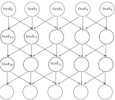
Stencil graph are composed of only one kind of task like in [BBR01]. Two other main information describe this graph: the width and the depth. Hence, there arewidth tasks composing the head of the graph and width tasks composing the tail. Except for these ones, a task have two or three fathers and two or three daughter. Next, we will refer to the task which is on thePSfrag replacements ith line and jth column by the task ij, the first task is noted (0,0).

task1 task2 taskn

head tail

Figure 5. A 1D mesh application composed of n tasks

Table 2 summarizes all the scenarios that we have investigated. One can see that we have performed 10 dif-ferent scenarios from (a) to (j). A scenario consists in the submission of applications and/or independent tasks.

(14)

type machine processor speed memory swap system server spinnaker xeon 2 GHz 1 Go 2 Go linux

artimon pentium IV 1.7 GHz 512 Mo 1024 Mo linux pulney xeon 1.4 GHz 256 Mo 533 Mo linux cabestan pentium III 500 MHz 192 Mo 400Mo linux valette pentium II 400 MHz 128 Mo 126 Mo linux chamagne pentium II 330 MHz 512 Mo 134 Mo linux soyotte sparc Ultra-1 64 Mo 188 Mo SunOS

fonck sparc Ultra-1 64 Mo 188 Mo SunOS agent xrousse pentium II bipro 400 MHz 512 Mo 512 Mo linux client zanzibar pentium III 550 MHz 256 Mo 500 Mo linux

Table 3. Resources of the testbed

size of the memory need (Mo) phase time in seconds

square matrix input output pulney artimon cabestan chamagne input sending time 3 3 4 4 1200 21.97 10.98 computing time 14 18 70 149

output sending time 1 1 1 1 input sending time 5 5 5 6 1500 34.33 17.16 computing time 25 33 136 292

output sending time 1 1 2 2 input sending time 7 8 8 8 1800 49.43 24.72 computing time 40 53 231 504

output sending time 2 2 3 3

Table 4. Dgemm tasks’ needs

parameter phase time in seconds

spinnaker artimon cabestan valette soyotte fonck input sending time 0.09 0.12 0.1 0.08 0.10 0.16 200 computing time 16 17.1 74.86 97.81 128.09 127.56

output sending time 0.05 0.03 0.03 0.03 0.06 0.05 input sending time 0.14 0.13 0.09 0.08 0.18 0.16 400 computing time 30.6 33.2 148.48 182.52 255.56 254.09

output sending time 0.06 0.03 0.03 0.03 0.06 0.05 input sending time 0.09 0.14 0.08 0.13 0.14 0.16 600 computing time 45.6 49.4 222.26 273.28 382.5 380.66

output sending time 0.05 0.03 0.03 0.03 0.06 0.05

Table 5. Wastecpu tasks’ needs

The number of clients gives the number of applications involved in a scenario. The definition of the DAG of an application is given in the form width per depth. Information are given on independent tasks when some are submitted during the execution of applications. Their number and the rate at which they arrive (the inter-arrival time is drawn from a Poisson distribution). Each scenario is composed of nbseeds different experiments that are executed nbrun times from where no variation in the results is observed. Finally, the total number of tasks in-volved in a scenario is given.

The following modalities are true for each set of experiments:

• The platform is made of one client, one agent and the number of servers is held to 4. The name of the servers registered to the agent is given in the corresponding subsection. The reader can refer to Table 3

(15)

PSfrag replacements

task0 task1 task2 task3 task4

task10 task11

task20 taskij

Figure 6. 5x4 stencil task graph

to have further information on the platform resources. We callheterogeneity coefficient of the platform, the maximum on all servers and on all tasks of the division of the maximum computing need by the minimum computing need for the same task, e.g. maxtaski

maxserversdi,s

minserversdi,s ;

• Only one kind of task (dgemm or wastecpu) is used to generate all the submitted applications in a scenario. Moreover, the same experiment has been carried out several times (equal to nbrun given in Table 2). This is referred to as arun. Results are means on these runs ;

• There is 3 different possible sizes when a task of a given type is drawn. Then, one can generate 3n_different

applications composed of n tasks ;

• We note that in each experiment of each scenario, a scheduling decision cost is negligible compared to the duration of the shortest task (less than 0.1 second) for all the proposed heuristics.

5.2. Scenarios (a) and (b): Submission of 500 Independent Tasks

We present two kind of submissions with scenario (a) and (b): the first scenario is composed of dgemm tasks and the second is made of wastecpu tasks. As we consider in this paper three possible inputs, one can generate 3500_{different sets of independent tasks for one experiment in each scenario. Given a generated set of tasks, the}

difference between two arrival dates is drawn from a Poisson distribution with a mean of µ = 20 seconds and µ = 15seconds.

In the following, we describe more precisely the two scenarios then we explain the results.

5.2.1 Scenario (a): Dgemm Independent Tasks Submission

In the first set of experiments, the tasks are multiplications of square matrix (dgemm) of size 1200, 1500 and 1800 leading to different time and memory cost (Table 4). The platform, described next, has an heterogeneous coefficient equal to 504/40 = 12.6. For all the experiments, the testbed is composed of:

• client: zanzibar ; • agent: xrousse ;

(16)

NetSolve’s MCT HMCT MP MSF number of completed tasks 500 500 500 500 makespan 9906 9908 10162 9905 sumflow 25922 19934 26383 19702 maxflow 230 103 517 97 maxstretch 12.8 5.8 3.7 5.3 percentage of

tasks that finish - 65% 66% 65% sooner than with

NetSolve’s MCT

Table 6. Scenario (a): results in seconds forµ = 20sec for dgemm Tasks

NetSolve’s MCT HMCT MP MSF number of completed tasks 495 358 500 500 makespan 7880 5600 7648 7626 sumflow 89254 25092 34677 31375 maxflow 1780 500 720 250 maxstretch 99 27.8 6.3 11.3 percentage of

tasks that finish - <85%> 84% 87% sooner than with

NetSolve’s MCT

Table 7. Scenario (a): results in seconds forµ = 15sec for dgemm Tasks • servers: chamagne ; pulney ; cabestan ; artimon.

Results on the makespan, the sumflow for µ = 20 seconds are given in Table 6 summarizes mean results for µ = 20seconds on the number of completed tasks, the makespan, the sumflow, the maxflow, the maxstretch and the percentage of tasks that finish sooner than if scheduled with MCT.

In Table 7, where µ = 15 and built the same way than the previous one, values for MCT and HMCT results are those obtained from the run when the number of completed tasks was the maximum. Indeed, for µ = 15, MCT and HMCT are not able to handle the throughput of tasks. HMCT and MCT overload the fastest servers that cannot accept any more jobs because they run out of memory. However, the NetSolve MCT has fault tolerance mechanisms that permit to schedule almost all tasks on some runs. For µ = 20, this phenomenon does not occur because the arrival rate lets faster servers complete more tasks before a new request.

One should note that for µ = 15 seconds, the NetSolve MCT gives very high values, and the highest for all the observed metrics, showing lesser performances. There is a huge time and space contention on the fastest servers. This is confirmed, for MCT and for HMCT, by the load average sent to the agent (more than 12 on pulney). Consequently, some servers collapsed during the experiment.

Even when there is low contention, e.g. when µ = 20 seconds, one can see from the results that using an heuristic that uses HTM information leads to better performances than MCT benefiting from load correction mechanisms. From these results, MSF is the best heuristic: it achieves the best performances regardless the metric and the rate of incoming submissions.

5.2.2 Scenario (b): Wastecpu Independent Tasks Submission

We use wastecpu tasks to prevent memory problems that we do not yet handle. The goal is to replace the multi-plication tasks, so its computation costs, dependent on the parameters, are similar to the multimulti-plication tasks. A wastecpu task can have the parameter 200, 400 or 600 which determines the time it costs (Table 5).

(17)

Two platform have been used. We give next the experimentations and the results obtained for each of them. For the both of them, we can remark with relief that two runs of the same experiment give slightly the same results. This explains the small number of experiments undertaken. Moreover, for this scenario, all tasks of each set have been submitted, accepted and computed by all of the five heuristics we have tested.

Platform 1 The heterogenous coefficient (the maximum computing cost divided by the minimum for the same

task) of the platform described next is 97/16 = 6. The experimental testbed for this set of experiments is made up of:

• client: zanzibar ; • agent: xrousse ;

• servers: valette ; spinnaker ; cabestan ; artimon.

We generated three different sets of tasks, submitted at two different arrival rates. Results for µ = 20 seconds, given in Table 9, are obtained from 2 executions of the same metatask scheduled by each of the four tested heuris-tics. At this rate, the experiment finishes after about 10, 000 seconds. In Table 8, for µ = 15 seconds, values are the mean of 4 executions for the NetSolve MCT and 3 for the three others. At this rate, the experiment needs about 7, 700 seconds to complete. For a set of independent tasks scheduled according to a given heuristic, the percentage of tasks that finish sooner is the mean of the values obtained from the comparison between each run for this heuristic and each run for NetSolve (hence obtained from a comparison in ‘cross product’). Finally, we give in the column ‘Avg’ the mean on the observed metric of the values obtained for each run and each set.

HMCT and MSF outperform MCT regardless the rate and the observed metric. If they give slightly the same results for µ = 20, MSF even outperforms HMCT when µ = 15 seconds. On the opposite, MP shows performance gains only for µ = 15 seconds. Our heuristics are specifically designed for environments with contention: gains increase with it.

(18)

NetSolve’s MCT HMCT MP MSF

seed1 seed2 seed3 Avg seed1 seed2 seed3 Avg seed1 seed2 seed3 Avg seed1 seed2 seed3 Avg

makespan 7690 7615 7644 7650 7655 7565 7626 7615 7672 7545 7765 7661 7672 7544 7626 7614 sumflow 63364 49529 50014 54302 39973 36675 34821 37156 33913 30860 30158 31644 34347 30279 29744 31457 maxflow 344 283 290 306 234 231 228 231 340 314 314 323 234 182 162 193 maxstretch 7.5 6.5 6.7 6.9 4.9 5 4.6 4.8 3.8 3.2 2.9 3.3 5 3.4 3.2 3.9 number of tasks that finish - - - − 78.6% 73.6% 77.6% 76.6% 83.2% 80.6% 82% 82% 84.6% 80.4% 82.4% 82.4%

sooner than with NetSolve’s MCT

Table 8. Scenario (b), platform 1: results in seconds forµ = 15sec for wastecpu Tasks

makespan 9913 10044 10210 10056 9901 10041 10210 10051 10009 10047 10265 10107 9903 10041 10209 10051

sumflow 25768 22036 20727 22844 20151 18151 17364 18555 26729 24384 24239 28451 20306 18138 17317 18587

maxflow 193 168 124 162 123 109 82 105 286 275 273 278 116 135 85 112

maxstretch 4.1 4.1 2.8 3.7 3.1 2.2 2.1 2.4 1.8 1.8 2 1.9 2.8 2.8 2.2 2.6

percentage of

tasks that finish - - - − 68.8% 62.8% 64.8% 65.4% 67.8% 63.4% 64.2% 65.2% 66.2% 61.8% 64% 64%

Table 9. Scenario (b), platform 1: results in seconds forµ = 20sec for wastecpu tasks

RR

n°

(19)

Platform 2 The heterogeneous coefficient of the second platform is slightly superior to the previous and equal

to 8.9. The following resources composed the environment: • client: zanzibar ;

• agent: xrousse ;

• servers: spinnaker, artimon, soyotte, fonck.

Three different seeds have been used to instantiate Scenario (b), and the resulting experiments have been sub-mitted at three different rates: 20, 17 and 15 seconds. For µ = 17 and µ = 20 seconds, each experiment has been submitted 3 times conducting to 9 submissions per rate and per heuristic for this scenario. For µ = 15 seconds, each experiment has been submitted 6 times then 15 submissions have been performed on the platform for this rate and for each heuristic. Tables presenting the results for µ = 20 are detailed next. Tables for µ = 17 and µ = 15 are built the same way.

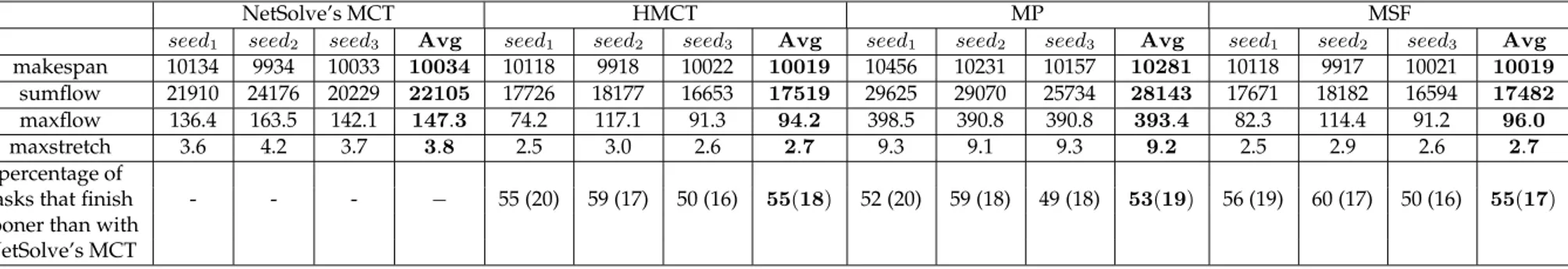
Results for the inter-arrival µ = 20 seconds are given in Tables 10, 11, 16. We describe in Table 10 the utilization of each server by each heuristic during each experiment: given an experiment, each percentage of allocated tasks on the 500 of the experiment (the corresponding part of each task type is precised in parenthesis) per server is given. The sumflow per server as well as the total sumflow that the experiment costs is also given.

Table 11 gives the mean flow recorded during the submission of the experiment scheduled by MCT and the average gain for each task type over MCT if the same experiment is scheduled by a given heuristic.

Table 16 summarizes many information: for each heuristic and each seed, mean results on the makespan, the sumflow, the maxflow, the maxstretch and the number of tasks finishing sooner than if scheduled by MCT are given.

Like for the previous platform, for each seed and each heuristic (naturally except MCT) the percentage of tasks that finish sooner is the average percentage obtained from the comparison of terminaison dates between each run for this heuristic and each run for NetSolve (hence from a comparison in ‘cross product’). A task is considered ‘finishing sooner’ if the terminaison dates differ from at least 2 seconds between MCT and the other heuristic. Thus, we give in parenthesis the percentage of tasks that finish sooner with MCT than with the given heuristic: because there exists tasks that finish in a range of 2 seconds between a run with MCT and with another heuristic, the sum of the percentage of tasks that finish sooner with our heuristic and the percentage of tasks that finish sooner with MCT differs from 100. Finally the column ‘Avg’ contains the mean on the observed metric of the values for each run and each seed.

The same experiments have been conducted with µ = 17 and µ = 15 seconds and we present the results re-spectively in Tables 12, 13, 17 and in Tables 14, 15, 18.

With Tables 10, 12 and 14, one can see the evolution of the processor utilization in function of the heuristic. Regardless the heuristic, the percentage of tasks scheduled on spinnaker decreases slightly: all types of tasks are concerned in the same manner. This benefits to the slower servers: only to artimon for HMCT, but MP and MSF give also more jobs to fonck and soyotte.

If HMCT and MSF have the same behavior and outperform both MP and MCT for µ = 20 and µ = 17, MP achieves to reduce the total sumflow progression and outperfom all the others for µ15 seconds.

Table 11 confirms that for slow rate, MP achieve sub-optimal scheduling. The average gain over MCT is neg-ative: each task scheduled by MCT is 28% shorter than with MP. On the opposite, at this rate, HMCT and MSF show nearly the same positive results: their scheduling leads to gain 20% on each task flow. Due to perturbations, when the rate increases to µ = 17 seconds, the average flow grows to 160% bigger with MCT. All of our heuristics outperfom MCT, HMCT and MSF maximising the gains for each task, allowing them to be 26% shorter. When the rate is high (µ = 15), MP achieves the best gains with an average flow 42% shorter than for MCT.

(20)

experiment 1

server MCT HMCT MP MSF

% of tasks sumflow % of tasks sumflow % of tasks sumflow % of tasks sumflow

spinnaker 56.9 (18.7 16.5 21.7) 12463 60.2 (19.6 18.0 22.6) 10344 52.6 (17.4 15.2 20.0) 8103 58.6 (19.4 16.8 22.4) 9959 artimon 43.1 (13.9 13.1 16.1) 9447 39.8 (13.0 11.6 15.2) 7381 35.2 (10.8 10.4 14.0) 6307 41.4 (13.2 12.8 15.4) 7712 soyotte 0.0 (0.0 0.0 0.0) 0 0.0 (0.0 0.0 0.0) 0 5.4 (1.6 1.8 2.0) 7185 0.0 (0.0 0.0 0.0) 0 fonck 0.0 (0.0 0.0 0.0) 0 0.0 (0.0 0.0 0.0) 0 6.8 (2.8 2.2 1.8) 8029 0.0 (0.0 0.0 0.0) 0 total sumflow 21910 17725 29624 17671 experiment 2 server MCT HMCT MP MSF

spinnaker 57.8 (21.7 19.9 16.2) 11307 61.3 (22.1 19.9 19.3) 9908 54.4 (19.8 17.4 17.2) 7907 59.6 (21.2 19.2 19.2) 9617 artimon 42.2 (14.3 14.1 13.8) 8922 38.7 (13.9 14.1 10.7) 6745 36.0 (12.6 13.8 9.6) 5809 40.4 (14.8 14.8 10.8) 6978 soyotte 0.0 (0.0 0.0 0.0) 0 0.0 (0.0 0.0 0.0) 0 4.0 (0.8 1.6 1.6) 5640 0.0 (0.0 0.0 0.0) 0 fonck 0.0 (0.0 0.0 0.0) 0 0.0 (0.0 0.0 0.0) 0 5.6 (2.8 1.2 1.6) 6377 0.0 (0.0 0.0 0.0) 0 total sumflow 20229 16653 25733 16595 MEAN server MCT HMCT MP MSF

spinnaker 57.3 (19.4 18.6 19.3) 12428 60.1 (19.8 19.7 20.6) 10149 53.1 (17.7 17.2 18.2) 7986 58.9 (19.8 18.9 20.2) 9859

artimon 42.7 (13.6 14.3 14.7) 9677 39.9 (13.3 13.2 13.4) 7369 36.1 (11.8 12.5 11.9) 6145 41.1 (13.3 14.0 13.8) 7623

soyotte 0.0 (0.0 0.0 0.0) 0 0.0 (0.0 0.0 0.0) 0 4.7 (1.1 1.7 1.9) 6580 0.0 (0.0 0.0 0.0) 0

fonck 0.0 (0.0 0.0 0.0) 0 0.0 (0.0 0.0 0.0) 0 6.1 (2.5 1.6 2.0) 7430 0.0 (0.0 0.0 0.0) 0

total sumflow 22105 17518 28142 17483

Table 10. Scenario (b), platform 2: processors utilization forµ = 20seconds

mean flow gain in percentage MCT (sec) HMCT MP MSF type 1 22.1 14.5 -44.9 14.9 experiment 1 type 2 42.6 20.8 -45.2 21.8 type 3 63.5 19.6 -27.1 19.4 type 1 23.2 21.5 -15.6 22.1 experiment 2 type 2 47.5 25.0 -6.6 24.9 type 3 71.7 25.6 -30.9 25.5 type 1 20.3 12.1 -35.8 11.8 experiment 3 type 2 41.1 18.6 -21.2 19.1 type 3 64.0 19.2 -28.3 19.5 MEAN - 44.0 19.7 -28.4 19.9

Table 11. Scenario (b), platform 2: average percentage gain forµ = 20sec on each task given by type

(21)

experiment 1

spinnaker 56.0 (18.9 18.3 18.8) 19370 55.1 (17.1 19.1 18.9) 14040 50.6 (17.4 16.8 16.3) 8477 54.5 (17.0 18.6 18.9) 13308

artimon 44.0 (14.2 14.6 15.2) 16009 44.9 (16.0 13.8 15.1) 11992 37.7 (11.6 12.0 14.1) 7503 45.1 (15.6 14.3 15.1) 12063

soyotte 0.0 (0.0 0.0 0.0) 0 0.0 (0.0 0.0 0.0) 0 6.0 (2.3 2.0 1.7) 7336 0.1 (0.1 0.0 0.0) 43

fonck 0.0 (0.0 0.0 0.0) 0 0.0 (0.0 0.0 0.0) 0 5.8 (1.8 2.0 2.0) 7639 0.4 (0.4 0.0 0.0) 258

total sumflow 35379 26031 30955 25672

Table 12. Scenario (b): processors utilization forµ = 17seconds

mean flow gain in percentage MCT (sec) HMCT MP MSF type 1 35.7 21.1 0.3 21.5 experiment 1 type 2 71.6 27.7 11.4 29.0 type 3 107.6 30.9 19.2 32.9 type 1 36.3 22.4 15.5 18.5 experiment 2 type 2 73.5 22.3 13.9 24.6 type 3 114.7 24.2 17.4 25.4 type 1 31.9 21.6 -1.9 22.3 experiment 3 type 2 59.6 27.2 -3.1 27.4 type 3 102.6 30.8 16.3 31.6 MEAN - 70.4 25.4 9.9 25.9

Table 13. Scenario (b), platform 2: average percentage gain formu = 17sec on each task given by type

(22)

experiment 1

spinnaker 53.3 (16.4 18.6 18.3) 38279 - - 49.3 (16.5 17.3 15.5) 13346 50.8 (14.4 18.0 18.4) 19274 artimon 44.8 (13.9 15.8 15.1) 33412 - - 40.2 (12.2 13.4 14.6) 12309 44.2 (13.0 15.4 15.8) 21121 soyotte 0.9 (0.1 0.5 0.3) 2468 - - 5.6 (1.2 2.7 1.7) 8409 2.0 (1.0 1.0 0.0) 2073 fonck 1.0 (0.2 0.3 0.4) 2695 - - 4.8 (0.7 1.8 2.4) 7996 3.0 (2.2 0.8 0.0) 2662 total sumflow 76854 - 42060 45130 experiment 3 server MCT HMCT MP MSF

spinnaker 55.0 (20.9 17.7 16.4) 25061 53.8 (19.1 18.8 15.9) 18870 47.7 (15.9 17.1 14.7) 9865 53.0 (18.2 19.3 15.5) 17279 artimon 45.0 (15.1 16.3 13.6) 21586 46.2 (16.9 15.2 14.1) 18181 41.2 (16.4 13.8 11.0) 9136 45.4 (16.5 14.5 14.5) 16303 soyotte 0.0 (0.0 0.0 0.0) 0 0.0 (0.0 0.0 0.0) 0 6.0 (2.6 1.6 1.8) 7562 0.7 (0.7 0.0 0.0) 465 fonck 0.0 (0.0 0.0 0.0) 0 0.0 (0.0 0.0 0.0) 0 5.1 (1.1 1.5 2.5) 7672 0.8 (0.6 0.2 0.0) 664 total sumflow 46647 34235 34711 MEAN server MCT HMCT MP MSF

spinnaker 53.8 (18.2 17.3 18.3) 35302 <52.0 (16.4 17.3 18.3)> <22497> 48.6 (16.4 16.2 16.0) 11710 51.1 (15.2 17.8 18.1) 18792

artimon 45.1 (14.6 15.2 15.3) 31304 <45.5 (15.4 14.5 15.6)> <23447> 40.5 (13.7 13.0 13.8) 10906 44.5 (14.4 14.2 15.9) 19007

soyotte 0.5 (0.1 0.2 0.2) 1054 <1.1 (1.1 0.0 0.0)> <716> 5.6 (1.6 2.2 1.8) 7907 2.0 (1.6 0.4 0.0) 1592

fonck 0.6 (0.2 0.2 0.2) 1213 <1.4 (1.4 0.0 0.0)> <946> 5.3 (1.4 1.5 2.4) 7917 2.4 (1.9 0.5 0.0) 1968

total sumflow 68873 <47605> 38439 41359

Table 14. Scenario (b): processors utilization forµ = 15seconds

mean flow gain in percentage MCT (sec) HMCT MP MSF type 1 83.6 18.7 52.4 31.7 experiment 1 type 2 162.8 31.6 51.1 47.2 type 3 234.5 31.8 53.2 50.2 type 1 67.7 - 48.0 28.2 experiment 2 type 2 151.6 - 42.2 40.0 type 3 230.7 - 46.3 45.4 type 1 51.8 19.7 31.7 23.3 experiment 3 type 2 95.3 23.7 35.1 30.3 type 3 144.0 20.4 19.8 25.7 MEAN - 135.8 <24.3> 42.2 35.8

Table 15. Scenario (b): average percentage gain forµ = 15sec on each task given by type

(23)

makespan 10134 9934 10033 10034 10118 9918 10022 10019 10456 10231 10157 10281 10118 9917 10021 10019

sumflow 21910 24176 20229 22105 17726 18177 16653 17519 29625 29070 25734 28143 17671 18182 16594 17482

maxflow 136.4 163.5 142.1 147.3 74.2 117.1 91.3 94.2 398.5 390.8 390.8 393.4 82.3 114.4 91.2 96.0

maxstretch 3.6 4.2 3.7 3.8 2.5 3.0 2.6 2.7 9.3 9.1 9.3 9.2 2.5 2.9 2.6 2.7

percentage of

tasks that finish - - - − 55 (20) 59 (17) 50 (16) 55(18) 52 (20) 59 (18) 49 (18) 53(19) 56 (19) 60 (17) 50 (16) 55(17)

Table 16. Scenario (b): results in seconds forµ = 20sec on wastecpu tasks

makespan 8525 8513 8557 8532 8513 8505 8517 8512 8831 8822 8825 8826 8500 8505 8517 8507

sumflow 36762 38105 31272 35380 26327 29235 22534 26032 31638 32039 29187 30955 25739 28920 22358 25672

maxflow 257.6 256.0 271.3 261.7 182.8 185.1 193.7 187.2 405.5 411.0 417.5 411.3 170.0 190.8 184.0 181.6

maxstretch 6.6 7.0 7.3 7.0 4.9 5.4 5.3 5.2 10.0 10.1 11.0 10.4 8.8 8.8 8.8 8.8

percentage of

tasks that finish - - - − 71 (19) 70 (20) 66 (19) 69(19) 75 (18) 74 (17) 67 (19) 72(18) 71 (18) 69 (20) 67 (19) 69(19)

makespan 7697 7677 7577 7650 7645 - 7551 7598 7910 7899 7844 7885 7646 7650 7546 7614

sumflow 83120 76854 46647 68874 58159 - 37051 47605 39024 42060 34236 38440 44235 45130 34712 41359

maxflow 420.1 883.4 323.0 542.2 313.1 - 288.6 300.8 441.2 521.8 430.1 464.4 264.5 348.0 264.1 292.2

maxstretch 10.3 23.8 8.5 14.2 10.6 - 7.2 8.9 11.8 14.9 12.4 13.0 10.2 12.8 9.6 10.8

percentage of

tasks that finish - - - − 84 (14) - 76 (20) 80(17) 87 (12) 84 (14) 82 (15) 84(14) 88 (11) 84 (14) 76 (20) 83(15)

(24)

5.2.3 Results

We have considered in this subsection the scheduling of a set of independent tasks whose inter-submissions fol-low a Poisson distribution of parameter µ equal to 15, 17 or 20 seconds. Therefore, the makespan is strongly dependent on the latest task arrival. We cannot expect at the very outset a big difference between two heuristics on that metric especially at low rate [MAS+_{99], even in a CPU shared environment. That is verified by our tests.}

Nonetheless, heuristics do not have the same performances.

The overall results converge even if gains are a bit better on the experiments performed on Platform 2: at the same rate, there is more contention as the heterogeneity increases. Thus our heuristics that are designed to take into account the contention behave even better.

One can note that MCT and HMCT tend to not use the slowest servers fonck and soyotte. Indeed, a task has to finish sooner on soyotte than on spinnaker to be scheduled there: this implies sufficient perturbations to do so, i.e. that during the execution of the task on spinnaker a number of tasks superior to the heterogeneity co-efficient be running concurrently for HMCT as well as an sufficient load on artimon as well. This clearly limits the throughput of tasks and even make HMCT unable to handle the second experiment on the platform 2 when µ = 15seconds.

To see how useful the HTM is, we compare results on the same heuristic: MCT and HMCT (in fact, these are not exactly the same due to NetSolve load correction mechanisms). We see in Table 9 that HMCT needs one missing hour (4289 seconds) of computations for a set of independent tasks whose time cost is of less than three hours (µ = 20) for the same makespan. Its performances are greater as the rate increases: a gain of 4.8 hours of computations for a duration of 2.1 hours, and there too, a better quality of service (Table 8).

Moreover, a better quality of service is offered regardless the rate: HMCT shows a gain in average response time in Tables 11, 13 and 15 but cases exist where it cannot handle the throughput of submissions. Results are always better for HMCT, and gains increase with the rate (see Tables 16, 17 and 18).

In consequence, the use of the HTM definitely leads to better results for Scenario (a) and (b), where the set of independent tasks can be perceived as one client with many tasks or many clients with at least one tasks.

MP has a better load balance property than MCT and HMCT (Table 9 and 8). Hence, when µ is large (low arrival rate), it loads slower servers because they are idle. Whereas, when µ is low, no servers are idle, then MP, like HMCT and MSF, tends also to load the fastest ones. MP presents the highest maxflow. It seems logical considering that:

• for µ = 20, as tasks on faster servers are not necessarily finished, slower servers are used. The MP maxflow comes from the maximum cost of a task on the slowest server.

• for µ = 15, there is contention even on the slowest servers. A task that had already a higher duration than if allocated to a faster server requires even more time.

Therefore at low rate, MP is sub-optimal, but is rather good at higher rates: less sumflow (even compared to MSF) and a high number of tasks that finish sooner than MCT.

MSF tries to optimize the sumflow, hence finds a good balance between minimizing the perturbation and minimizing the new task duration. Therefore, it gives good performances on the makespan, the sumflow, even on the maxflow and the percentage of tasks that finish sooner than with MCT is always very high (nearly the same than MP’s for µ = 15 !). While MSF is not explicitly designed to optimize the makespan as is MCT, it appears that it always outperforms MCT, as well as HMCT and MP on most of the metrics. Considering that an agent cannot guess the rate of the requests it will have to process, MSF is the best because it gives the same performances than HMCT at low rates and better performances than others at higher rates.

5.3. Scenario (c): Submission of 10 1D-mesh Applications, Each Composed of 50 Wastecpu Tasks

An experiment consists in the submission of 10 applications composed of 50 wastecpu tasks each. An applica-tion is a 1D-mesh applicaapplica-tion (secapplica-tion 5.1), hence, when a client has received the result of its task, he immediately

(25)

sends a new request to the agent until the last task: the tail of the application.

One can generate for each client 350_{applications. Tasks needs are given in Table 5. We assume that the}

differ-ence between two application head arrival dates (e.g. two client first submissions) follows a Poisson distribution with a mean of µ = 15 seconds.

Four experiments have been generated, each with a different seed. Then, two experiments differ from each other in the arrival date of each client head as well as in the composition of applications (see Table 19).

The same experiment has been executed 6 times. As we will explain, even on exactly the same experiment, an heuristic can have a non negligible standard deviation on its results.

The heterogeneity coefficient of the platform, equal to 273.28/45.6 = 8.9, is made of: • client: zanzibar ;

• agent: xrousse ;

• servers: spinnaker, artimon, soyotte, fonck.

client experiment 1 experiment 2 experiment 3 experiment 4 type 1 type 2 type 3 type 1 type 2 type 3 type 1 type 2 type 3 type 1 type 2 type 3 client 1 20 11 19 20 17 13 16 16 18 22 12 16 client 2 17 13 20 15 21 14 22 16 12 12 19 19 client 3 13 17 20 14 16 20 20 19 11 14 17 19 client 4 14 15 21 11 22 17 20 12 18 18 14 18 client 5 18 13 19 10 14 26 17 18 15 22 12 16 client 6 18 16 16 11 22 17 19 18 13 22 14 14 client 7 11 19 20 20 16 14 17 17 16 16 17 17 client 8 21 14 15 19 13 18 15 19 16 16 18 16 client 9 16 12 22 14 19 17 18 17 15 21 12 17 client 10 22 13 15 18 11 21 16 10 24 23 14 13 total 170 143 187 152 171 177 180 162 158 186 149 165

Table 19. Scenario (c): applications composition

0 1000 2000 3000 4000 5000 6000 7000 8000 9000 10 9 8 7 6 5 4 3 2 1 time (sec) client number MCT HMCT MP MSF

(26)

0 1000 2000 3000 4000 5000 6000 7000 8000 10 9 8 7 6 5 4 3 2 1 time (sec) client number MCT HMCT MP MSF

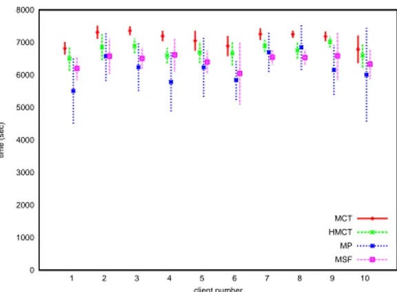
Figure 8. Scenario (c): Results on the makespan for the second experiment

We note that, at any time, all clients can have a request being computed in the distributed system. So, there is at most 10 tasks in the environment at a given moment.

Moreover, we must also note that, on the contrary of the previous section (submission of a set of independent tasks), scheduling decisions are not necessarily the same between two runs. With that kind of application, results can consequently differ between two runs. Indeed, the arrival date of a task can differ even slightly between two runs: a task can finish sooner or later than in another run. As precedence links exist, daughters might not be scheduled to same servers. This scenario leads immediately to a different run, especially if the scheduling heuristic has a tendency to use slower servers: all the next termination dates change due to scheduling decisions taken consequently to the system state, which differs. As all the tasks arrival dates of an application might differ, and due to the heterogeneity of the platform, the makespan for example can vary.

Figure 9. Scenario (c): results on the makespan for the third experiment

5.3.1 Results

The results of the 4 experiments are given in Figures 7, 8, 9, 10 and in Tables 20 and 21.

One can see in each graph the mean and the standard deviation of the makespan obtained on the 6 runs for each of the 10 submitted applications. As applications are 1D-mesh, we can consequently compare sumflows on these graphics if neglecting the head arrival date (due to the low value of head arrival dates, graphs are nearly identical). Indeed, for this kind of application, the makespan is the head arrival date added to the sumflow.

(27)

Figure 10. Scenario (c): results on the makespan for the fourth experiment

experiment 1

spinnaker 53.6 (18.5 16.5 18.6) 36932 47.5 (12.7 15.9 18.9) 27644 49.5 (18.1 15.2 16.2) 17270 45.9 (13.1 14.7 18.1) 21782

artimon 46.4 (15.9 14.8 15.7) 34630 42.3 (12.4 14.4 15.5) 31800 41.4 (14.9 13.0 13.5) 21716 39.7 (11.7 12.1 15.9) 26822

soyotte 0.0 (0.0 0.0 0.0) 0 4.7 (4.1 0.6 0.0) 3766 4.5 (0.7 1.5 2.3) 11522 7.0 (4.7 2.1 0.2) 7852

fonck 0.0 (0.0 0.0 0.0) 0 5.6 (5.2 0.4 0.0) 4346 4.6 (0.7 1.5 2.4) 11729 7.4 (5.0 2.3 0.2) 8198

total sumflow 71562 67556 62239 64654

Table 20. Scenario (c): processors utilization

Table 20 gives, for each experiment and each heuristic, the percentage of allocated tasks on the 500 of the experiment per server (the part of each task type is also specified in parenthesis), the sumflow per server and the total sumflow that has cost the execution of the whole experiment on the system.

(28)

makespan HMCT MP MSF experiment 1 5.5 13.3 9.7 experiment 2 5.4 13.0 9.8 experiment 3 6.1 12.4 9.0 experiment 4 5.1 13.0 9.5 MEAN 5.5 12.9 9.5 sumflow HMCT MP MSF 5.6 13.4 9.9 5.4 13.2 9.9 6.2 12.6 9.1 5.1 13.1 9.6 5.6 13.1 9.6

Table 21. Scenario (c): average percentage gain against MCT on the makespan and the sumflow for each client

Finally, Table 21 gives for each experiment and each heuristic, the average percentage that each application gains on the makespan and on the sumflow against if scheduled with MCT. One should note that gains on the sumflow that can be red in this table are close to those on the makespan (as expected), and of course, can differ from the one that can be computed from Table 20 where they would be gains on the whole experiment, e.g. ex-periment resource consumption benefices.

At first, we can note that MCT does not, or hardly, use the slowest servers (Table 20). This can lead to high con-tention on the fastest servers and delay the termination date of each tasks, then the makespan of each application. In fact, for each experiment, using the HTM leads to better performances and each application finishes sooner than when MCT schedules the experiment. MP seems to be the heuristic that leads to the best results, whatever metric is regarded : makespan, sumflow, average gain, but MP has also a considerable standard deviation, and a greater number of run has not proven to reduce it (mainly due to the use of the slowest servers, as it is explained below).

Indeed, whichever experiment MP schedules, it leads to better performances on the makespan and on the sumflow: a greater number of application finish sooner than when the experiment is scheduled with another heuristic, the average gain on the makespan (and so for the sumflow) for each application is around 13% against MCT, compared to 5% for HMCT and 9% for MSF (Table 21).

MP uses the slowest servers for the longest tasks, as opposed to MSF (Table 20) which tends to use the slowest for short tasks. We can also note that MP allocates less tasks to the slowest servers than the other, but as longest tasks cost the most, it leads to a greater sumflow on these servers and a lesser on the fastest.

The standard deviation on the makespan grows with the quantity of tasks mapped on the slowest servers and their type: MCT has a low standard deviation, HMCT a small one. It uses slow server, but for short tasks. MSF uses them also for tasks of second type and consequently its client makespan has a bigger standard deviation. MP has the biggest, using them mainly for long tasks.

Using the HTM leads to a better use of the system resources: the experiment sumflow is always inferior than MCT’s (more than 13% if MP is used). Moreover, If we consider that each resource has a proportional cost to its power, then our heuristics, especially MP, would make an financial profit of much more than 13% because less expensive resources are the most solicited.

But, one should note that the utilization of resources with our heuristics can be sub-optimal: when only one application subsists (e.g. only sequential jobs remain), we have observed that our heuristics do not necessarily use the fastest server, due to the model/reality synchronization.