Conceptual design of adaptive structural control systems

Conceptual Design of Adaptive Structural Control Systems

by

Michael Cusack

B.S. Civil Engineering

Rensselaer Polytechnic Institute, 1998

Submitted to the Department of Civil and Environmental Engineering

in partial fulfillment of the requirements for the degree of

Master of Science in Civil and Environmental Engineering

at the

MASSACHUSETTS INSTITUTE OF TECHNOLOGY

September 1999

@ Massachusetts Institute of Technology 1999. All rights reserved.

A uthor

Department of Civil and Environmental Engineering

August 6, 1999

~1(

72

Certified by...

Jerome J. Connor

Professor

Thesis Supervisor

72

Accepted by...

..-Conceptual Design of Adaptive Structural Control Systems

by

Michael Cusack

Submitted to the Department of Civil and Environmental Engineering on August 6, 1999, in partial fulfillment of the

requirements for the degree of

Master of Science in Civil and Environmental Engineering

Abstract

Civil engineering structures have long been at the mercy of extreme events, such as earthquakes and high winds. But recently the process of structural control has allowed engineers to affect how structures behave during extreme events, improving the performance of the structures under these conditions. Passive structural control systems are effective at limiting the response to a narrow spectrum of excitations, but they can do little to control the response outside of this spectrum. Active structural control differs from passive structural control in that it relies on external energy to achieve a higher level of control. Active structural control systems allow a structure to analyze its current state, decide on the appropriate corrective actions, and implement these actions through control forces, which translates to improved performance over a wider range of excitations. Although practical applications of active structural control have been demonstrated in actual structures, their use has been limited because of the large energy requirements of the system.

This thesis explores the concept of adaptive structural control, a special type of active structural control. By controlling a system adaptively, one changes the stiffness and damping of the system, as well as the gain of the control algorithm, to affect the response. This varying of parameters, combined with the use of smaller actuator forces, can result in a better overall performance of the structure, while using much less energy.

Three different proposed systems of control force-generating actuators are presented. In addition, a simulation of non-adaptive active structural control and adaptive structural control on a single degree of freedom system is presented. The intent is not only to show the superior performance of the controlled system over the uncontrolled system, but also to demonstrate the appropriateness of adaptive structural control as an alternative to non-adaptive active structural control.

Thesis Supervisor: Jerome J. Connor

Acknowledgements

First, many thanks go to my advisor, Jerome Connor, who has taught me more in the last year than I could have thought possible. After having access to his vast knowledge, I am a little wiser going into the real world and have a newfound appreciation for the opportunities that lie ahead. His guidance and patience in helping me complete my thesis was immeasurable.

Secondly, I thank my sister Eileen, and my brothers Patrick, Timothy and Kevin. They are some of the best friends I have ever known and it has been very rewarding to watch them grow up. Because of them, life on Hickory Road has always been unpredictable and fun.

Finally, and most importantly, I thank my parents, who truly made all of this possible. They have been there for me my whole life, and they always believed in me, even the times when I didn't believe in myself. Thanks to them, and everything they have ever given me, I finally made it.

Contents

1

1.1 Definition of Active Structural Control ... 13

1.2 Com ponents of Active Structural Control System ... 13

1.3 Active Control and Adaptive Control ... 14

1.4 Scope of Thesis ... 14

Actuator Technologies

2.1 Theory ... 15

2.2 Com ponents of Leveraging System ... 16

2.2.1 Colum n A ssem bly... 16

2.2.2 W all A ssem bly ... 17

2.2.3 D iagonal A ssem bly ... 20

2.2.4 M ulti-Story A ssem bly ... 21

2.3 M aintenance Issues ... 22

2.4 Production of Actuator Units ... 22

2.5 M aterials... 23

2.5.1 H igh-Strength Steel... 23

2.5.2 Com posite M aterials ... 23

2.6 Section G eom etry of Lever Arm s ... 24

2.7 Robustness ... 24

2.8 Optim izing D isplacem ent and Force Output... 24

2.9 Optim al Layout of Actuators ... 25

3 Electrom agnetic Force System ... 26

3.1 Theory ... 26

3.2 M agnetic Levitation (M aglev) System ... 27

3.2.1 Electrom agnetic Suspension System ... 27

3.2.2 Levitation Capacity of Electromagnetic Maglev Vehicles ... 27

3.2.4 Levitation Capacity of Electrodynamic Maglev Vehicles ... 29

3.3 Com ponents of Electrom agnetic System ... 29

3.3.1 Solenoids ... 29

3.3.2 Rotating D isc... 30

3.3.3 Casing... 31

3.4 Superconducting Coils ... 31

3.4.1 Tem perature Control ... 31

3.4.2 Quenching ... 32

3.5 Problem s w ith M agnetic Fields... 32

3.5.1 Interaction w ith Structural Steel... 32

3.5.2 Interaction with Hum an W orking Space... 32

3.6 Elem ent Configuration ... 33

3.6.1 Size of Com ponents ... 33

3.6.2 Placem ent of Elem ents... 34

3.7 Power Requirem ents ... 35

3.8 M aintenance ... 36

3.9 Cost of Electrom agnetic System ... 36

3.10 Custom ized U nits Versus Standardized Units ... 37

4 Pulley A ctuating System ... 38

4.1 Theory of Tension M agnification ... 38

4.2 Cable Locations... 41

4.3 Cable M aterials ... 42

4.4 Access and M aintenance ... 42

4.5 Optim ization... 43

Algorithms

5.2 Determination of Optimal Control Force... 46

5.3 Stability of Active Control Algorithm ... 49

5.3.1 Stability of the Physical System... 49

5.3.2 Stability of the Physical System with Continuous Active Control ... 50

5.3.3 Stability of the Physical System with Discrete Active Control ... 51

5.3.4 Time Delay Effects on Discrete Active Control Algorithm... 51

5.4 Examples of Active Control Systems ... 53

5.4.1 Active Mass Driver ... 53

5.4.2 Active-Passive Composite Tuned Mass Damper... 55

5.4.3 Hybrid Pendulum Damper ... 55

5.5 Principles of Adaptive Structural Control... 56

5.5.1 Variable Stiffness System ... 56

5.5.2 Variable Damping System ... 57

5.5.3 Electrorheological (ER) Fluids ... 58

5.5.4 Magnetorheological (MR) Fluids... 59

6 Control Algorithms Applied to a Single Degree of Freedom System ... 60

6.1 System Parameters ... ... 60

6.2 Active Control Algorithm...- ... ... 61

6.2.1 Sinusoidal Ground Motion... 61

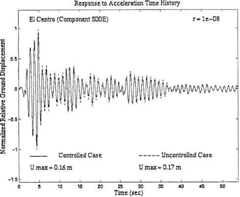
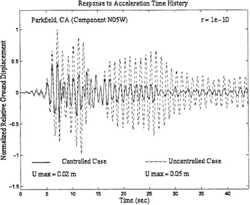
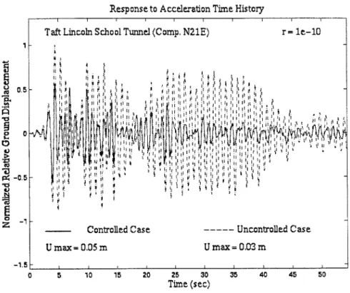
6.2.2 Earthquake Time Histories... 63

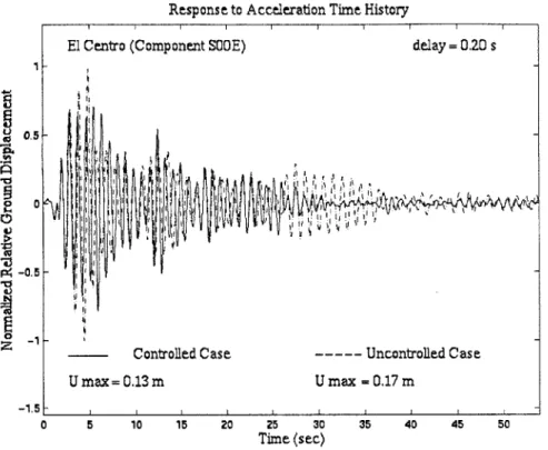
6.2.3 Time Delay Effects ... 65

6.3 Adaptive Control Algorithm... 66

6.3.1 Adaptive Control Versus Active Control... 66

6.3.2 Modifications to the Adaptive Control Algorithm... 67

6.3.3 Calculation of Adaptive Stiffness ... 69

6.3.4 Calculation of Adaptive Damping ... 72

6.3.5 Distribution of Control Force... 73

6.3.6 Results for Adaptive Case...77

6.3.7 Stability of the Adaptive Control Algorithm ... 81

6.3.8 Time Delay Effects on the Adaptive Control Algorithm... 81

7.1 Discussion ... 83 7.2 Further Development ... 83 Appendix A ... 84 Appendix B...91 Appendix C ... 103 Appendix D ... 116 Appendix E...133 Appendix F...144

List of Figures

2.1 Column Assembly Actuator ... 17

2.2 Lever Assemblage Inside Wall Panel... 18

2.3 Lever Assemblage Inside Wall Panel (Shear Control)... 19

2.4 Shear Lever Assemblage Acting on Building ... 20

2.5 Diagonal Actuating Assembly... 20

2.6 Multi-Story Actuating Assembly ... 22

3.1 Schematic Representation of Magnet... 34

3.2 Electromagnet in (a) Column and (b) Beam... 35

4 .1 S im ple P ulley ... 3 8 4.2 1-Degree Compound Pulley ... 38

4.3 Multi-Degree Compound Pulley ... 39

4.4 Incorporation of Intermediate Reactions into Control Tension... 40

4.5 Schematic of Pulley System in Tall Building... 41

4.6 Schematic of Compound Pulley System in Tall Building... 44

5.1 Schematic Representation of Active Structural Control ... 45

5.2 Stiffness Types for A V D ... 57

6.1 Response to Sinusoidal Ground Motion, r = 1 x 10-9... . . . 62

6.2 (a) Single Degree of Freedom System... 76

6.2 (b) Free B ody D iagram ... 76

6.3 Free Body Diagram for Adaptively Controlled SDOF System... 77

6.4 Response to El Centro Time History, r = 1 x 10-9 (Adaptive Control) ... 79

6.5 Time History of Variable Stiffness for El Centro Excitation, r = 1 x 10-9 ... 79

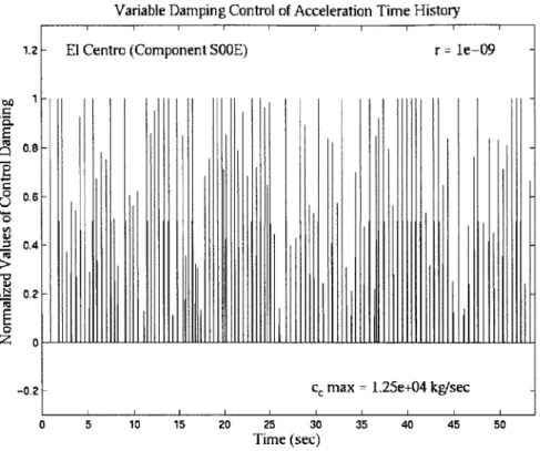
6.6 Time History of Variable Damping for El Centro Excitation, r = 1 x 10-9 ... 80

6.7 Time History of Control Force for El Centro Excitation, r = 1 x 10-9... 80

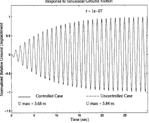
Al Response to Sinusoidal Ground Motion, r = l x 10-7... 87

A2 Time History of Control Force for Sinusoidal Ground Motion, r = 1 x 10-...87

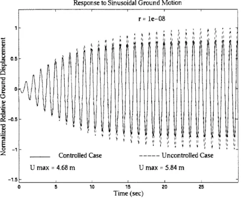
A3 Response to Sinusoidal Ground Motion, r = 1 x 10-8... 88

A5 Response to Sinusoidal Ground Motion, r = 1 x 10-9... ... . . . 89

A6 Time History of Control Force for Sinusoidal Ground Motion, r = 1 x 10-9...89

A7 Response to Sinusoidal Ground Motion, r = 1 x 10-10 ... 90

A8 Time History of Control Force for Sinusoidal Ground Motion, r = 1 x 1010 ... 90

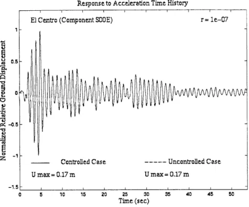
B1 Response to El Centro Time History, r = 1 x 10-7... 94

B2 Time History of Control Force for El Centro Excitation, r = 1 x 10~7... 94

B3 Response to El Centro Time History, r = 1 x 10-8... 95

B4 Time History of Control Force for El Centro Excitation, r = 1 x 10~8... 95

B5 Response to El Centro Time History, r = 1 x 10~9... 96

B6 Time History of Control Force for El Centro Excitation, r = 1 x 10-9... 96

B7 Response to El Centro Time History, r = 1 x 10-10... 97

B8 Time History of Control Force for El Centro Excitation, r = 1 x 1010 ... 97

B9 Response to Helena, MT Carroll College Time History ... 98

B 10 Time History of Control Force for Helena, MT Carroll College Excitation... 98

B 11 Response to Olympia Western, WA Time History ... 99

B 12 Time History of Control Force for Olympia Western, WA Excitation... 99

B 13 Response to Parkfield, CA Time History ... 100

B 14 Time History of Control Force for Parkfield, CA Excitation... 100

B 15 Response to San Francisco Golden Gate Time History ... 101

B 16 Time History of Control Force for San Francisco Golden Gate Excitation... 101

B 17 Response to Taft Lincoln School Tunnel Time History... 102

B 18 Time History of Control Force for Taft Lincoln School Tunnel Excitation ... 102

Cl Response to El Centro Time History, td = 0.02 sec ... 106

C2 Time History of Control Force for El Centro Excitation, td = 0.02 sec... 106

C3 Response to El Centro Time History, td = 0.20 sec ... 107

C4 Time History of Control Force for El Centro Excitation, td = 0.20 sec... 107

C5 Response to El Centro Time History, td = 0.22 sec ... 108

C6 Time History of Control Force for El Centro Excitation, td = 0.22 sec... 108

C7 Response to El Centro Time History, td = 0.24 sec ... 109

C10 Time History of Control Force for El Centro Excitation, td = 0.26 sec... 110

C1I Response to Helena, MT Carroll College Time History, td = 0.24 sec ... 111

C12 Response to Helena, MT Carroll College Time History, td = 0.26 sec ... 111

C13 Response to Olympia Western, WA Time History, td = 0.24 sec ... 112

C14 Response to Olympia Western, WA Time History, td = 0.26 sec ... 112

C15 Response to Parkfield, CA Time History, td = 0.24 sec ... 113

C16 Response to Parkfield, CA Time History, td = 0.26 sec ... 113

C17 Response to San Francisco Golden Gate Time History, td = 0.24 sec... 114

C18 Response to San Francisco Golden Gate Time History, td = 0.26 sec... 114

C19 Response to Taft Lincoln School Tunnel Time History, td = 0.24 sec... 115

C20 Response to Taft Lincoln School Tunnel Time History, td = 0.26 sec ... 115

D 1 Response to El Centro Time History, r = 1 x 10-7... 121

D2 Time History of Variable Stiffness for El Centro Excitation, r = 1 x 10~7 ... 121

D3 Time History of Variable Damping for El Centro Excitation, r = 1 x 10-7 ... . . . 122

D4 Time History of Control Force for El Centro Excitation, r = 1 x 10-7... 122

D5 Stability Check of Adaptive Control Algorithm for El Centro Excitation... 123

D6 Response to El Centro Time History, r = 1 x 10-8... 124

D7 Time History of Variable Stiffness for El Centro Excitation, r =1 x 10-8 ....--- .124

D8 Time History of Variable Damping for El Centro Excitation, r = 1 x 10~8 ... 125

D9 Time History of Control Force for El Centro Excitation, r = 1 x 10-8... 125

D10 Stability Check of Adaptive Control Algorithm for El Centro Excitation... 126

DI1 Response to El Centro Time History, r = 1 x 10-9 . . . . 127

D12 Time History of Variable Stiffness for El Centro Excitation, r = 1 x 10-9... ... 127

D13 Time History of Variable Damping for El Centro Excitation, r = 1 x 10~9_... ... ₁₂₈

D14 Time History of Control Force for El Centro Excitation, r = 1 x 10-9 ... 128

D15 Stability Check of Adaptive Control Algorithm for El Centro Excitation... 129

D 16 Response to El Centro Time History, r = 1 x 10-10 ... 130

D17 Time History of Variable Stiffness for El Centro Excitation, r = 1 x 10-10... 130

D18 Time History of Variable Damping for El Centro Excitation, r = 1 x 1040... 131

D19 Time History of Control Force for El Centro Excitation, r = l x 10-10 ... 131

E l Response to El Centro Time History, td = 0.24 sec ... 138

E2 Response to El Centro Time History, td = 0.26 sec ... 138

E3 Response to Helena, MT Carroll College Time History, td = 0.24 sec ... 139

E4 Response to Helena, MT Carroll College Time History, td = 0.26 sec ... 139

E5 Response to Olympia Western, WA Time History, td = 0.24 sec ... 140

E6 Response to Olympia Western, WA Time History, td = 0.26 sec ... 140

E7 Response to Parkfield, CA Time History, td = 0.24 sec ... 141

E8 Response to Parkfield, CA Time History, td = 0.26 sec ... 141

E9 Response to San Francisco Golden Gate Time History, td = 0.24 sec... 142

ElO Response to San Francisco Golden Gate Time History, td = 0.26 sec... 142

E 11 Response to Taft Lincoln School Tunnel Time History, td = 0.24 sec ... 143

E12 Response to Taft Lincoln School Tunnel Time History, td = 0.26 sec ... 143

F1 Change in Maximum Allowable Time Delay with Varying Stiffness ... 145

F2 Change in Maximum Allowable Time Delay with Varying Damping ... 145

List of Tables

3.1 Capacities and Clearances for Electromagnetic Systems... 27

3.2 Capacities and Clearances for Electrodynamic Systems... 29

6.1 Values of System Parameters for Control Simulation... 60

6.2 Changes in Response and Control Force with Changing r... 62

6.3 Earthquake Time Histories Used in Control Simulations ... 63

6.4 Summary of Response to El Centro Time History ... 64

6.5 Response of System to Various Time Histories ... 64

6.6 Response of System to Time Delay Effects for Varying r ... 66

6.7 Magnitudes of Force Terms for Adaptive Control... 76

6.8 Summary of Response to El Centro Time History (Non-Adaptive Control)...78

6.9 Summary of Response to El Centro Time History (Adaptive Control) ... 78

1 Introduction

1.1 Definition of Active Structural Control

Active structural control is the process of altering the response of a structure by application of external forces. The intent in altering the response of the structure is to limit the structure's response to a prescribed level. Applications of active structural control exist in areas of high seismic activity, where large ground accelerations can literally shake buildings to pieces, and areas of high winds, where tall buildings are subjected to significant dynamic loads. By applying control forces, one can limit the effect that the excitations have on the structure. This has come of interest in recent years, as the concept of performance of structures has taken on new importance. Whereas in the past buildings were designed so that they would not collapse during an earthquake, oftentimes now it is required that they remain operational after an earthquake, with minimal damage to critical components. Such needs merit having structures that can react to the loads they undergo, so that they can survive and remain functional.

1.2 Components of Active Structural Control System

In general terms, an active structural control system consists of components that measure the state of the system, decide on a course of action to take, and implement that course of action. Sensors capable of recording displacement, velocity, or acceleration at a given time measure the state of the system. How many of these sensors are installed and where they are placed will affect the degree of measurement of the current state. A central computer acting as a cognitive unit for the control system typically carries out decision-making processes. By examining the current state of the system, it decides what forces to apply to minimize the response. Implementation of these control forces is done by force actuators, which are capable of producing large forces through mechanical, magnetic, hydraulic or other processes.

1.3 Active Control and Adaptive Control

An active structural control system is one that uses external energy to affect the response of the system. This is in contrast to passive structural control, which requires no external energy. Adaptive structural control is a form of active structural control, where the structural system changes its stiffness and damping to adjust its response. This self-adjusting of stiffness and damping leads to a control algorithm that varies with time; in other words, the gain of the control algorithm is no longer constant. With non-adaptive active control, there is no change in the gain of the control algorithm. In order for adaptive control to be considered an effective alternative to non-adaptive active control however, it must be shown that a similar magnitude of control can be achieved using either method.

1.4 Scope of Thesis

This thesis presents the conceptual design of three high-force actuator systems to implement active structural control in civil engineering structures. Additionally, it presents a detailed breakdown of the theory behind active and adaptive structural control, and summarizes a computer simulation of active and adaptive control on a single degree of freedom system. The objective of these simulations is to demonstrate the effectiveness of adaptive structural control

as an alternative to active structural control.

Chapter 1 introduced the idea of structural control, and the basic definitions of active and adaptive structural control. Chapter 2 presents a conceptual system of high-force actuators that use large pliers-like elements to magnify actuator forces going into the system. Chapter 3 shows a similar type of system where actuator forces are generated by superconducting electromagnets. Chapter 4 details a high-force actuator system using large cables to control motion. Chapter 5 discusses the theory behind active structural control. Chapter 6 summarizes the active control and adaptive control simulations and presents the theoretical basis for the adaptive control algorithm. Finally, the conclusions are presented in Chapter 7.

2 Mechanical Leveraging System

2.1 Theory

As its name implies, this system operates on the principle of mechanical leverage. The concept is to use actuators to create small forces that can then be translated into larger actuating forces through plier or scissor action to generate the necessary effect on the structure. The unit is intended to be packaged so that it will fit inside a single column or a single wall and could be mass-produced in predetermined sizes and force ratios, unless it appears to be more economical to design the leveraging elements on an individual basis. The basic mechanical principle is as

follows:

Pin x rin = Pt x ro, , (2.1)

where Pi, is the force input to the system from the actuator, rin is the lever arm from the input force to the pivot point of the system, and similarly Pout is the output force, and rout is the lever

arm associated with the output force. One can rearrange (2.1) to solve for the output force:

P.ut = P X j. (2.2)

rout)

Assuming one wants to keep the actuator (input) forces as small as possible, which will result in energy savings, the way to increase the output force is to increase the length of the lever arm of the input force relative to the lever arm of the output force. If this mechanism is installed vertically in a typical story of a typical building, one can expect to achieve a maximum ratio of ri,/rout of about 10:1. Furthermore, if this output force can be coupled to another identical leveraging mechanism and used as input, called Pint (for intermediate force), then additional magnification of the original input force can be realized, along with greater energy savings. The final output force is now

Pou, = Pi. im in rn xin , (2.3)

n . (2.4)

Since for every iteration it is possible to achieve force magnifications on the order of 10:1, it may be possible to get total magnifications on the order of 100:1, a substantial increase in force. This would allow for the use of conventional force actuators and small linear motors to provide input forces, whereas previously these actuators would not have had the capacity to be effective in controlling civil engineering structures.

2.2

Components of Leveraging System

2.2.1 Column Assembly

The column itself will be designed somewhat like a space truss, and will be required to resist all gravity loads and lateral loads. (See Figure 2.1.) Incorporation of the leveraging system will require that as much as possible of the interior column space remain open, hence the space truss concept (Fig. 2.la). The system components will essentially look like a large pair of pliers inside the column (Fig. 2.1b), with the long lever arms coupled with the input forces and the shorter arms coupled with the output forces. It will not be the function of the pliers to resist any "normal" loads on the column; their sole purpose will be for providing control forces.

Depending on how many of these pliers are coupled together, the input force actuators will either be located at the top or bottom of the column assembly. They will apply forces to the long arms in the transverse direction, which will cause the arms to open or close, depending on the direction of the input force. The subsequent moment action around the pivot point in the assembly and through the short arms on the opposite end of the assembly will provide a magnification of the force. Although originally applied in the transverse direction, the force can easily be converted to an axial force (Fig. 2.lc). As the longer lever arms close, the smaller lever arms will rotate and push against a rigid plate welded to the top of the space truss. This plate will transmit axial forces to the column.

In addition to damping out the structure's response to dynamic excitation, the column actuator assemblies will also have the capacity to resist short-term gravity loads applied to the structure

which are in excess of the structural capacity of the passive column elements. Depending on the use of the structure, this feature may or may not be advantageous. If for example, these column actuators were installed in a warehouse, then it would be possible to occasionally permit heavy equipment or other such large loads to occupy the floor area for short periods of time at non-regular intervals. This type of adaptive prestressing would enable the columns to resist compression by inducing tension. Ordinarily it would be prohibitively expensive to design a structure to resist extreme loads such as this, but by making use of actuator technology, it would be possible to do this on occasion. Such an operation, however, would require a failsafe system and necessitate severe precautions to insure the safety of all those in the area. If such operations were to take place, it would require a very high degree of robustness in the system, an issue to be discussed later.

Force transfer to plate

Rigid Plate

uator Force _{Column Edge}

(a) (b) (c)

Figure 2.1 -Column Assembly Actuator - (a) Space truss-like structural frame, (b) lever components inside column, (c) close-up of top of column-plate interface

2.2.2

Wall Assembly

mostly within the horizontal plane, instead of the vertical plane, and is done through more simple lever action, rather than scissor or plier action. By using the spacing between two adjacent column lines, it could be possible to achieve force magnifications greater than the 10:1 ratio predicted for the column assembly, depending on the size of the bay. Also, this system may allow for more instances of force coupling and force magnification, due to the availability of vertical space, out of the plane of the lever action.

Ideally, the output force will be tied into an exterior column, where it will be most efficient. The final stage lever can be welded, or preferably bolted, to the top of the column through a plate or brackets positioned near the top of the column. Bolted connections are preferred to welded connections because bolted connections would prevent any moments from being imparted to the column. There may be, however, transmission of lateral forces to the top of the column, if the lever motion is not completely vertical. This can be minimized by keeping the upper lever arm as horizontal as possible, as shown in the figure below.

Free Joint Fixed Joints

A B

Figure 2.2 - Lever Assemblage Inside Wall Panel

The system works as follows. (Refer to Figure 2.2.) An input force is provided at point A, which causes the lower lever arm to rotate around point B, which is fixed in space. Point C is a freely moving hinge that transmits forces from the lower lever to the upper lever. The motion of

the lower lever arm causes point C to move upwards, rotating the upper lever arm around point

D, which is fixed in space. This transmits a compressive load to the column.

Much like the column assembly, this mechanism could be used to provide resistance to extreme static gravity loads as discussed in the previous section. The issue of robustness again becomes central, as this procedure should not be carried out if the performance of the system cannot be guaranteed.

Another option, to control shear deformation with a wall assembly, is to position the elements in a typical story as shown below.

Chevron Brace

I Input Force

Rigid Link

Figure 2.3 - Lever Assemblage Inside Wall Panel (Shear Control)

An input force P1 is applied to the top lever arms of the pliers in the right bay. The reaction in

the lower right lever arm, P2, is transmitted to a pin connection at the base. The reaction in the

lower left lever arm (also P2) is transmitted to a rigid link that is attached to a Chevron brace in

the left bay. The Chevron brace then transmits the lateral force in the rigid link to the top of the bay as a shear force.

/7/

Figure 2.4 - Shear Lever Assemblage Acting on Building

2.2.3 Diagonal Assembly

In addition to the previous proposal, another option for controlling shear deformation is configuring the system so that forces are generated along the diagonals of a bay, as shown:

Figure 2.5 - Diagonal Actuating Assembly

P2

P-Conceptually, this arrangement is no different than the previous, except for the orientation of the pliers. Instead of being tied to a Chevron brace, the pliers can push or pull against the T-shaped brace elements along the diagonals to generate shear forces. Because of symmetry, the same output force can be supplied by applying half the same input force in each pair of pliers, which will allow for use of smaller, cheaper actuators. An offset to this advantage however, is the somewhat limited space in the diagonals of the bay, which may force the lever arms to be smaller than desired. This will require an increase in the actuator forces, as well as stiffening of the lever arms.

2.2.4 Multi-Story Assembly

In order to increase lever arm ratios to maximize force magnification, it is prudent to explore the possibility of extending lever components through multiple stories. With this arrangement will come some loss of the dispersed control offered by many smaller elements, but a greater range of control forces will be gained, which will allow for control of the structure over a larger range of applied loads. In addition, because fewer elements will need to be manufactured for the structure, there exists the potential for cost savings. There are actually two separate ways in which output forces applied to the structure can be increased with a multi-story system. One is that the lever arm ratio can be made much higher, due to the increase in available space. The other is that because a larger system will be inherently stronger, it will be able to handle larger input forces, which lead to larger output forces. In order to work properly however, this system will need to make use of a Chevron brace similar to the one in Figure 2.3.

Figure 2.6 - Multi-Story Actuating Assembly

2.3 Maintenance Issues

Because this system will involve many moving parts, routine maintenance will be required to insure proper functioning of the unit. Of specific interest will be the proper lubrication of the pivot joints around which the levers will turn. Furthermore, the levers themselves will need to be monitored, since they will undergo several bending cycles during their lifetime. One possibility for monitoring is the attachment of strain gages to the lever arms to establish a response history of the lever arms. Because these units will be, for the most part, inaccessible once installed, it would make sense to have some kind of intelligent monitoring system as part of the leveraging unit itself. This way the system will "know" when it needs to be serviced, and the proper maintenance can be carried out.

2.4 Production of Actuator Units

Whether the leveraging units become a mass-produced item, with certain sizes available to designers, or else designed on a job to job basis will depend largely on the quantity of their use,

and the variation in loads they must supply. From a design standpoint, it may make more sense for structural engineers to have access to standard prefabricated units with available specifications, to help speed up the design process. Furthermore, designing the structural assembly which will house the actuating components will be a time-consuming task, and will make the units more expensive if it needs to be carried out for every job.

Of course, it would not be reasonable to exclude the possibility of large custom designed

mod-ules for "once in a lifetime" jobs that may develop. The limiting size of the actuating units will depend on the strength of the leveraging arms and how much force magnification can be provided, which will be a function of the available space within the structure. Convention suggests that as the loads increase the size of the structural elements housing the pliers and components of the force actuators will have to increase, but this may not necessarily mean more available space for actuator components.

2.5

Materials

2.5.1 High-Strength Steel

The leveraging systems presently being discussed will be required to create forces large enough to control axial deformations in steel and concrete. Therefore, to design the leveraging arms and joints out of conventional steel will not make a lot of sense, since those materials will undergo deformations along with the structural elements, which will limit the effectiveness of the leveraging system. Any material that is used will need to be very resistant to bending, so that the lever effect that takes place within the unit remains as efficient as possible. A sufficient choice of material would be a high-strength steel which possesses a rigidity greater than that of the structural steel in place, so that induced deformations take place in the structure, and not in the leveraging components themselves.

system on the overall weight of the structure. Typically this type of material costs much more than steel, but much of the increased unit cost can be gained back because of the substantially lower weight of the composite materials. Furthermore, once the loading conditions for the lever elements are known, the composite sections can be engineered more precisely, increasing their overall efficiency.

2.6 Section Geometry of Lever Arms

In addition to making the material as strong as possible, the efficiency of the unit will be increased as the inertia of the leveraging arms is increased to resist deflections due to bending. The leveraging arms could be conceived as resembling mini wide-flange shapes, which will provide stiffness in the primary bending direction and additional stiffness in the weak axis direction, enhancing the stability of the lever arms.

2.7 Robustness

In the case of extreme events, maintaining power to the actuating elements is critical to the operation of the control system. It is recommended that the power system used to control the actuating elements be given special consideration and possibly be entirely separate from the power supply for the remainder of the structure. But it should also be able to draw from a dedicated generator, which should be kept at the highest level of operation standards, in preparation for a major seismic event. Rigorous testing of the system components under harsh conditions is the only way to make any relevant claims as to the robustness of the system. Even then, there are certainly no guarantees of performance once the system is in place, which suggests that active control technology may not yet be mature enough to handle life-critical situations.

2.8 Optimizing Displacement and Force Output

As the amount of force magnification increases within a unit, the amount that the same unit can displace decreases proportionately. For example, if at the input end of a leveraging unit, the ends of the lever arms can be moved 10 cm and the force magnification is 10:1, then the amount that the lever arms will be able to move at the output end is 1 centimeter. As the lever arm ratio is increased, the amount the output lever arms move will become smaller and smaller. At some point, it will no longer be practical to magnify the output force by increasing the lever arm ratio. Conversely, if larger output displacements are desired, the amount that the lever arms move at the input end will need to become accordingly larger. Obviously, the size of the unit will restrict how large the displacements can be at the input end, but a compromise will need to be reached between the amount of output force that is generated and how much the lever ends can move. How this trade-off is settled will depend on the size of the forces required for control, the sizes of the available actuators and the expected movement of the structure.

2.9 Optimal Layout of Actuators

Where the actuators are placed in the building will be a function of the cost of the actuators, what level of force can be provided, and what constraints exist to limit installation. In theory, one would like to have actuators along every diagonal and along every column line, to provide complete localized control. In reality however, cost constraints will usually prevent one from achieving this type of dispersed control. Therefore, the best solution would be to place the actuators in the locations where they will have the largest effect.

For example, in the case of bending of a tall, slender structure due to wind loads, the largest axial forces will occur at the outside faces of the structure at the base. This would be the best place to install force actuators, since they can offset the largest amount of bending moment that way. Similarly, if one wanted to control shear deformation in a structure caused by seismic motion, the most useful place to install the actuators would be where the shear deformation is a

3 Electromagnetic Force System

Electromagnets are capable of generating large forces, large enough to be used for lifting and levitating heavy objects. The idea to use electromagnets to create forces in beams and moments in columns borrows from the technology behind many types of high-speed "maglev" (magnetic levitation) trains used throughout the world. During operation, these trains are levitated through magnetic attraction or repulsion between individually controlled electromagnets fitted to the vehicle and on the guideway. Through an electronic control system, a roughly constant separation distance between the guideway and the bottom of the train is maintained at all times.

3.1 Theory

Electromagnets employ currents to create magnetic fields. Consider a wire with some current moving through it and an identical wire with the same current moving through it placed parallel to the first wire at some distance away from it. The two wires will generate either an attractive or repulsive force, depending on which way the currents are moving. If the currents are moving in the same direction, they will attract; if they are moving in opposite directions, they will repel. The same idea can be extended to a loop of wire. If now two identical loops of wire are placed one on top of the other, and identical currents are sent through each wire in opposite directions, then a repulsive force will be generated between the two loops. If the force between the two loops is equal to or greater than the weight of the top loop, then the repulsive force between the loops will levitate the top loop.

Obviously this is an unstable arrangement and the top loop will likely fall to the ground since it is not supported laterally. But this demonstrates the theory of magnetic levitation and shows how magnetic forces can be used in structural control schemes.

If multiple loops of wire (known as a solenoid) are used instead of a single loop of wire, much

larger magnetic fields can be generated; this will increase the force. Assuming that lateral movements can be constrained, it will be quite easy for one solenoid to repel the other one in a

single direction. If the current in either solenoid can be varied, then the magnetic field and force between the solenoids can be controlled as well, and the system is now active.

3.2 Magnetic Levitation (Maglev) System

3.2.1 Electromagnetic Suspension System

This type of system uses the forces of magnetic attraction between electromagnets on the bottom of the vehicle and iron or aluminum plates on the vehicle guideway. Each electromagnet on the vehicle is typically a solenoid with an iron core, which is then used to interact with the metal plates on the guideway. In this case the attractive force between the two elements must be con-trolled, by varying the current supplied to the electromagnet. Determination of the current is done through monitoring the separation gap between the elements, usually maintained between

10 and 15 mm [1].

3.2.2 Levitation Capacity of Electromagnetic Maglev Vehicles

The table below lists the capacities of the electromagnets used on several different types of magnetic levitation vehicles [1, 2]. In presenting this information it must be remembered that each system has a different definition of what a "magnet" is, i.e. how many solenoids are included in each unit. (For the remainder of this chapter, the terms "coil", "magnet", "electromagnet", and "solenoid" will be used interchangeably.) The capacities shown below are per coil, to provide a means of comparison among the various systems. The gaps indicate the effective gap between the vehicle and the guide rails.

MAGLEV System Capacity (kN) Gap (mm)

Birmingham 9.8 15

HSST 8.3 9

Transrapid 18.7 8

U. Tokyo / Fuji (Model A) 5.3 10

Although these forces are not on the order to control large civil engineering structures, they do show that sizeable forces can be realized through magnetic technology. One can envision using these magnets to control "light" civil structures, such as transmission towers. Or, these magnets could be used in multiple numbers to generate larger forces, as is done with maglev vehicles. Furthermore, these magnets could be used as the driving actuators for the pliers-like actuators presented in the previous chapter. Nevertheless, one must not disregard magnetic technology because of the seemingly small forces it produces. Rather, one must recognize the potential in further developing this technology to generate larger forces, and the applications that currently exist.

3.2.3 Electrodynamic Suspension System

During this type of suspension, repulsive forces are created through induction occurring between on-board magnets (induction coils) and ground conductors during operation of the vehicle. Only the ground conductors have current supplied to them. The ground coils are placed along the sides of the track in a vertical "figure-8" shape so that the magnetic fields in each loop are of opposite polarity. Each induction coil is aligned on the side of the vehicle, vertically off-center from the ground coil, so that as it is moved past the ground coil, it experiences a net magnetic field which induces current in it. The induced magnetic field in the vehicle magnet is always such that the magnet is attracted to the top loop of the "figure-8" ground coil and repulsed by the bottom loop, creating a net levitation force [3].

The Canadian Maglev System uses a different type of electrodynamic induction system, which employs current-carrying electromagnets on the vehicle and a conducting sheet or surface laid out on the track. If an electromagnet moves over the conducting surface at some distance d / 2, the conducting sheet will make it appear as if a second electromagnet exists at some distance d from the electromagnet on the vehicle, and will generate a repulsive force. In some cases rows of ground coils are used in place of the conducting surface, but the principle is essentially the same. When the vehicle electromagnets are moved over the ground coils, current is induced in the ground coils and a repulsive force is generated [4].

3.2.4 Levitation Capacity of Electrodynamic Maglev Vehicles

Force capacities and effective gap lengths for four prototype electrodynamic maglev systems are shown in Table 3.2. Capacities are per coil [1, 4, 5, 6].

MAGLEV System Capacity (kN) Gap (mm)

MLUOO1 12.3 100

MLU002 13.9 110

MLU002N 15.5 Not available

Canadian Maglev 30 220

Table 3.2 - Capacities and Clearances for Electrodynamic Systems

As was the case with the electromagnetic systems, the electrodynamic coils do not appear to have force levels large enough to control civil engineering structures. However, they do show a noticeable increase over the values exhibited by the electromagnetic systems, thereby possessing even more potential. The greater problem becomes then how to install this type of magnetic system within a building or other similar structure, since the coils need to be moving to generate magnetic forces. Section 3.3.2 will attempt to deal with this problem.

3.3 Components of Electromagnetic System

3.3.1 Solenoids

As stated, the magnets themselves are actually solenoids, a series of wire loops designed to amplify the magnetic effects of current flowing through the wire. As the number of loops in the solenoid increases, the magnetomotive force, an indicator of the magnetic field strength of the solenoid, increases accordingly:

Typically, magnetomotive force is reported in amperes or ampere-turns. Solenoids used in prototype maglev operations have typically had magnetomotive forces of several hundred kilo amperes [5].

Even with such an arrangement, however, it is difficult to generate appreciably large forces because of the resistance of the conducting wire. An attempt to use a simple solenoid to create forces large enough to be used in civil structures or even in maglev operations would require enormously large input voltages, which would be expensive, unsafe, and possibly unrealizable. This problem has been avoided, however, through the use of superconducting materials, which are capable of conducting electricity while offering very low (near zero) resistance. This is achieved by operating the superconducting wires at temperatures near absolute zero. (Typical operating temperatures in maglev superconducting magnets are around 4.5-5 K [7].) Under these conditions, it is possible to achieve large magnetomotive force by using "conventional" voltages, which will lead to magnetic forces that are large enough to be effective.

It is anticipated that the actuating electromagnets will make use of superconducting technology. The best arrangement of the superconducting magnets will be to use them in pairs, so that they can either repel each other, or else attract each other. Each magnet will be tied to the surrounding structural elements, so that the forces generated between the two magnets can be transferred to the structure.

3.3.2 Rotating Disc

Another possibility of creating the individual actuators will involve using only one magnet combined with a rotating disc made of a conducting material. It was mentioned previously that electrodynamic maglev operations do not use two current-carrying electromagnets to achieve levitation, but use one current-carrying electromagnet in conjunction with a conducting sheet, which creates a levitation force when the elements move past each other at a sufficient velocity. The proposed arrangement would situate a single current-carrying electromagnet over a disc made of a conducting material. When the system is not in use, the electromagnet will rest some small distance above the disc, so not contact is made when the unit shuts down. But when the system goes into use, power will be supplied to the electromagnet and the disc will rotate

underneath it, which will create the same effect as the electromagnet moving over a conducting surface.

As the speed of the disc increases, the levitation force will also increase. Maglev trains usually run at operating speeds of around 300 to 500 km/hr, which for a 0.5-m diameter disc would translate into a rotational speed of 3200 to 5300 rpm. This could result in substantial power savings because current will only need to be supplied to one electromagnet in each unit. Of course, the idea of putting a motor within a structural element will not be easily perfected, but could be a very economically attractive choice.

3.3.3 Casing

The casing to house the magnetic components should be such that it allows the components of the system to be packaged as a single unit. Ideally, the units would arrive to the jobsite prepackaged and ready to install. The casing structure should add minimal weight to the unit, suggesting composites as a reasonable choice of material from which to build the casing. The weight of the unit must be kept as small as possible so that installation of a unit requires a minimum number of workers.

3.4 Superconducting Coils

3.4.1 Temperature Control

One of the main problems with using superconducting elements is the required operating temperature of superconductors is around 4.5 K, near the boiling point of helium. Because of this, superconductors require extensive cooling to remain operational, usually through piping in a fluid like liquid helium to keep the coils cold [7]. Doing this will consume large amounts of energy, and will also lessen the robustness of the system because a large power source will need to be maintained at all times to keep the system operational. Supplying a cooling system

3.4.2 Quenching

Superconductors are also very prone to quenching (loss of superconducting properties due to excessive heating) because of their low heat capacity, which requires very little input heat to trigger a quench. The source for this heat is often mechanical disturbances within the coil matrix [7]. Because the coils will be subject to significant motion during an earthquake, the problem of quenching becomes very serious, since one cannot afford to have the coils quench as soon as an earthquake starts. The best method of limiting these disturbances is to restrain wire movement within the coil matrix.

3.5

Problems with Magnetic Fields

3.5.1 Interaction with Structural Steel

Steel is of course a conducting material, and could pose a problem to the use of magnetic actuators, because the steel has the potential to disrupt the magnetic flux between the elements of the electromagnetic unit. To alleviate this problem, the structural steel will need to be "separated" from the magnets, through some kind of shielding that prevents magnetic fields from flowing through the structural steel. Covering every piece of steel in the structure with shielding could be prohibitively expensive, so it may prove more prudent to isolate the magnetic components from the structural steel by shielding the exterior of the actuator. In either case, careful attention must be paid to the efficiency of the system and how it varies with the type of shielding provided. This situation could eventually lead to an optimization problem between the loss in efficiency and the increase in cost from shielding.

3.5.2 Interaction with Human Working Space

This problem is very similar to the one encountered in maglev systems, where the concern is over large magnets situated very close to passengers. It is also an extension of the shielding problem that needs to be addressed for the structural steel, and may be solved through the same means. Magnetic fields decrease in magnitude very significantly as they move away from their

source (proportional to 1/r2_{) and most likely will pose no threat to office workers who reside in}

close proximity to the magnetic units in a building. If it appears that undesirable magnetic fields could be produced in the working area then shielding will be required.

3.6 Element Configuration

3.6.1 Size of Components

Obviously, the smaller the physical size of the actuators, the more attractive they become, since they can be located in a larger variety of places within structural elements. Most of the maglev systems that have been built to date have used very large coils, usually 1.5-2 m long by 0.5-1 m in height, with a thickness of about 0.25 m [3, 5, 6]. However, these magnets are usually made up of more than one coil and could be broken down into smaller elements if necessary. When looking at the design variables of the electromagnets, it becomes apparent that the size of the loops in the superconducting solenoids should be made as small as possible, so that the magnet can fit within a beam or column. This will tend to decrease the available magnetic field because the length of wire in each loop will be smaller. However, this loss can be made up in a few ways. One is to simply increase the number of loops, which will increase the magnetomotive force of the coil. Another is to increase the power supplied to the electromagnet, although this solution should be considered a last resort since power usage should be kept to a minimum. If the single magnet / rotating disc arrangement is considered, the problem provides a little more flexibility in terms of what parameters can be adjusted, but it also presents more constraints on size. In addition to the superconducting coils needing to be as small as possible, the rotating disc and motor will also need to be made sufficiently small to fit inside the structural compo-nents. One way of adapting to the problem is, as in the previous solution, to increase the number of loops in the superconducting coil. Another is to increase the speed of the rotating disc, although this has its drawbacks because it will require additional power input, plus beyond a certain speed of the disc there will be no additional levitating force generated.

3.6.2 Placement of Elements

Two different systems incorporating this technology are proposed. The first is to attach electro-magnets to a column to create either compressive or tensile axial forces. The other is to use sets of magnets located along the top and bottom flanges of a beam to generate edge axial forces that will translate into bending moments in the beam.

The idea of installing electromagnets on a column is fairly straightforward. Considering the column to be a standard wide-flange shape, a total of two electromagnets will be placed on the column, in pairs near the middle of each "channel" created by the flanges and web. The exact location and size of these electromagnets will depend on the amount of power necessary to control the electromagnets and how that power requirement varies with the size of the electromagnets. In either case, the electromagnets should be placed symmetrically about the beam to insure that no eccentric loads are created when the electromagnets are activated, or even so that no eccentricities are developed under the dead weight of the electromagnets. In addition to the magnet arrangements proposed in previous sections, a single magnet arrangement, as shown in Figure 3.1, could also be used.

Each solenoid will have a metal rod inserted in its core. As a current passes through the solenoid, the metal bar will move. By restraining the motion of the solenoid and the bar, the magnetic force can be transmitted to the beam or column.

Metal Bar

Solenoid

For the beam elements, the arrangement is very similar except, as mentioned, electromagnets are located along the inside of the top and bottom flanges of the beam, assuming that the beam is a wide-flange shape. The forces are applied in the same manner as in the column, with each pair of electromagnets generating either a compressive or tensile force. But unlike in the column arrangement, if the electromagnets on the top flange generate a compressive force, the electromagnets on the bottom flange will create a tensile force, so as to create an overall bending moment in the beam. On the opposite side of the beam, the electromagnets will be used to generate the same forces, so that no eccentricity is induced in the beam and the beam bends about its major axis. It should be noted that this arrangement could also be used to generate weak-axis moments, and could also be used to create twisting in the beam to combat torsional effects.

*7

(a) (b)

Figure 3.2 - Electromagnets in (a) Column and (b) Beam

noids are, and the more loops they have, the better, since they will generate more magnetomotive force and larger fields for the same input voltage. Nonetheless, the system is going to require substantial forces to be of any use, so it will need larger currents in order to generate those forces. A more complete analysis of the power requirements would involve examining the requirements of superconductors under various conditions.

3.8 Maintenance

The electromagnetic force actuator system is considerably complex and could suffer breakdowns in several components. As with other actuator systems, one will need to consider the frequency with which components will need replacement and decide on what access should be made available to those components. In this respect, maglev systems can be studied to determine what kind of maintenance was required of them during their operational lifetime, since the electromagnets in this situation will undergo a similar course of operation and will be comprised of similar components.

3.9 Cost of Electromagnetic System

The largest barrier to entry of implementing an electromagnetic actuator system most likely will be the substantial cost associated with the cooling subsystem required for the superconducting coils. However, recent research in maglev technology has experimented with using permanent magnets in place of electromagnets, which would eliminate the need for cooling. Use of permanent magnets had been considered unfeasible in the past because permanent magnets could not produce forces large enough to offset their enormous weight. But by using a configuration known as the Halbach array, the magnets can be placed in such a way that concentrates the power of the magnets in one direction, increasing the force capacity [8]. Use of this technology in actuator systems would eliminate the need for superconductors and drive down the cost of the system.

3.10 Customized Units Versus Standardized Units

Initially, these units are going to be manufactured on an individual, customized basis, since there will be no previous uses of this technology from which to adapt. As the system develops, it may be beneficial to compromise between customizing and standardizing by having units standardized by size but with interchangeable components. For example, the solenoids that are used in the assembly can be interchangeable so that different magnetomotive forces can be selected based on the system requirements. Similarly, for the rotating disc arrangement, the disc diameter could be a standardized parameter, but the system could be supplied with different motors to supply the necessary speeds, depending on how much speed is needed and how precise the control has to be. In addition, as mentioned previously, different conducting materials could be available for the rotating disc to satisfy system requirements.

4 Pulley Actuating System

4.1 Theory of Tension Magnification

Pulleys have been long been used to aid in lifting heavy objects. One pulley by itself can be used to reverse the direction of motion of a cable so that lifting becomes a pulling-down motion, one that is usually easier to implement than pulling up, since it can use gravity to its advantage. If one considers the pulley and weight arrangement shown below in Figure 4.1, the tension in the cable is equal to the weight of the object, T = W.

T

Figure 4.1 - Simple Pulley

But if a second pulley is added to the system, as shown below, the same weight can be lifted and held in equilibrium by a reduced amount of tension in the cable. In this case, T is now equal to W/ 2, so the required tension is cut in half.

T

Figure 4.2 - 1-Degree Compound Pulley

In general, if pulleys are added to the system in this manner, the tension required to hold the weight in equilibrium will decrease as the number of pulleys increases, and will be calculated by the following equation:

W

T= - (4.1)

2x

w

Figure 4.3 - Multi-Degree Compound Pulley

where, x is the total number of pulleys minus 1. So for example, if the system were set up in such a way to include 11 total pulleys, the required tension to maintain equilibrium would be

W W

T , (4.2)

210 1024

which means that it the weight to be sustained is 1 kN, the required tension in the cable to hold the weight in place will be about 1 N. This arrangement rapidly demonstrates its usefulness in civil engineering structures, where small input forces can be increased in such a way as to provide effective control of large structures through force actuation.

This system offers yet additional advantages in its method of force magnification, demonstrated