HAL Id: hal-01105390
https://hal.archives-ouvertes.fr/hal-01105390
Submitted on 20 Jan 2015
HAL is a multi-disciplinary open access
archive for the deposit and dissemination of
sci-entific research documents, whether they are
pub-lished or not. The documents may come from
teaching and research institutions in France or
abroad, or from public or private research centers.
L’archive ouverte pluridisciplinaire HAL, est
destinée au dépôt et à la diffusion de documents
scientifiques de niveau recherche, publiés ou non,
émanant des établissements d’enseignement et de
recherche français ou étrangers, des laboratoires
publics ou privés.
Dynamics of a thin liquid film interacting with an
oscillating nano-probe
René Ledesma-Alonso, Philippe Tordjeman, Dominique Legendre
To cite this version:
René Ledesma-Alonso, Philippe Tordjeman, Dominique Legendre. Dynamics of a thin liquid film
interacting with an oscillating nano-probe. Ethnopolitics, Taylor & Francis (Routledge), 2014, vol. 10
(n° 39), pp. 7736-7752. �10.1039/c4sm01152j�. �hal-01105390�
To cite this
this version : Ledesma-Alonso, René and Tordjeman,
Philippe and Legendre, Dominique Dynamics of a thin liquid film
interacting with an oscillating nano-probe. (2014) Soft Matter, vol.
10 (n° 39). pp. 7736-7752. ISSN 1744-683X
O
pen
A
rchive
T
OULOUSE
A
rchive
O
uverte (
OATAO
)
OATAO is an open access repository that collects the work of Toulouse researchers and
makes it freely available over the web where possible.
This is an author-deposited version published in :
http://oatao.univ-toulouse.fr/
Eprints ID :
12288
To link to this article :
DOI:10.1039/c4sm01152j
http://dx.doi.org/10.1039/c4sm01152j
Any correspondance concerning this service should be sent to the repository
administrator:
staff-oatao@listes-diff.inp-toulouse.fr
Dynamics of a thin liquid film interacting with an
oscillating nano-probe
Ren´e Ledesma-Alonso,* Philippe Tordjeman and Dominique Legendre
The dynamic interaction between a local probe and a viscous liquid film, which provokes the deformation of the latter, has been studied. The pressure difference across the air–liquid interface is calculated with a modified Young–Laplace equation, which takes into account the effects of gravity, surface tension, and liquid film–substrate and probe–liquid attractive interaction potentials. This pressure difference is injected into the lubrication approximation equation, in order to depict the evolution of a viscous thin-film. Additionally, a simple periodic function is added to an average separation distance, in order to define the probe motion. The aforementioned coupled equations, which describe the liquid film dynamics, were analysed and numerically solved. The liquid surface undergoes a periodic motion: the approaching probe provides an input energy to the film, which is stored by the latter by increasing its surface deformation; afterwards, when the probe moves away, an energy dissipation process occurs as the surface attempts to recover its original flat shape. Asymptotic regimes of the film surface oscillation are discerned, for extreme probe oscillation frequencies, and several length, wavenumber and time scales are yielded from our analysis, which is based on the Hankel transform. For a given probe–liquid– substrate system, with well-known physical and geometric parameters, a periodic stationary regime and instantaneous and delayed probe wetting events are discerned from the numerical results, depending on the combination of oscillation parameters. Our results provide an interpretation of the probe–liquidfilm coupling phenomenon, which occurs whenever an AFM test is performed over a liquid sample.
1
Introduction
Over the past two decades, the application of dynamic mode atomic force microscopy (AFM) techniques has become a current practice for scanning so matter samples.1
Neverthe-less, the choice of AFM imaging mode should be made carefully in order to prevent inconveniences and undesired phenomena. Indeed, whenever a probe is brought into close proximity to a surface, molecules jump from the surface to the probe2due to
the attractive van der Waals tip sample interaction. This state-ment has been extensively discussed1,3,4and observed
experi-mentally, when a probe is brought close to a high temperature solid sample5,6
and to polymeric liquid lms.7,8As a probe
quasi-statically approaches a liquid sample, or a liquid layer deposited over a solid substrate, the liquid surface performs a jump towards the probe at a minimum separation distance.9–11The
intermittent contact mode (IC-AFM) reduces the probe–sample interaction time, by oscillating the probe in the vicinity of the sample surface and provoking a so probe–sample contact. Images of liquid droplets using IC-AFM had been obtained,12,13
also registering a large phase contrast when the probe–liquid
contact occurs, which indicates the presence of an energy dissipation phenomenon. Indeed, every time the probe comes close to the liquid sample surface, a capillary neck forms between the probe and the sample.14,15This may cause as well
the liquid volume to split into two parts, one remaining as the sample and the other placed over the probe surface.
Imaging of the droplet prole using non-contact mode (NC-AFM), which avoids the probe–liquid contact, has been shown as a possible solution.1,16–22A recipe to obtain good resolution
topographies, consisting of the use of an oscillation frequency about 100 Hz higher than the cantilever resonance frequency, a free oscillation amplitude of around 10 nm and a probe–sample distance between 22 and 50 nm, which is heuristically deter-mined, has been recently exposed and successfully employed.20,21,23If larger amplitudes or shorter probe–sample
distances are used, an “accidental” contact between the tip and the sample is provoked and, as a consequence, distorted droplet proles are captured. Although the proposed methodology provides quality results, a formal justication of this experi-mental combination of parameters still remains to be revealed. Despite the non-intrusive nature of NC-AFM, the surface of a so sample encounters the growth of a nano-protuberance under the action of the oscillating probe.24Using a Kelvin–Voigt
viscoelastic material to model the so sample, in which inertial effects are disregarded, and a forced non-linear damped
Universit´e de Toulouse, INPT-CNRS, Institut de M´ecanique des Fluides de Toulouse (IMFT), 1 All´ee du Professeur Camille Soula, 31400 Toulouse, France. E-mail: rledesma@im.fr; Tel: +33 05 3432 2802
oscillator, including a sphere/at surface interaction force, to mimic the NC-AFM operation,25 the sample deformation is
estimated aer the model parameters are determined by tting experimental data. When NC-AFM experiments are performed, it is advisable to use stiff cantilevers, which provides cantilever deection stability, and to minimize the probe–liquid separa-tion distance, which increases the probe sensitivity, in order to accomplish true atomic resolution. In this scenario, the suitable scanning parameters must be dened to prevent the probe–so sample contact and the loss of the original shape of the sample and shrinking of volume. Therefore, the NC-AFM jump-to-contact distance and the sample surface deformation should be deduced and compared to those for a static probe–liquid interaction.
In this paper, we present a theoretical and numerical study of the liquid lm dynamics, generated by its interaction with an oscillating nano-probe. First, in Section II, we present equations that describe the probe and lm dynamics. In Section III, we describe an implemented pseudo-spectral method to solve the probe–lm dynamics. Section IV is devoted to the results of the numerical simulations, performed for different probe oscilla-tion condioscilla-tions. In Secoscilla-tion V, we submit a theoretical analysis in the wavenumber domain and a solution for the lm surface position. Section VI reports the critical oscillation parameters that lead to the probe wetting. Finally, in Section VII we discuss the consequences of the probe–liquid dynamic coupling on AFM experimental situations.
2
Problem formulation
A liquid lm of thickness E, density r, dynamic viscosity m and air–liquid surface tension g deposited over a at horizontal substrate, as shown in Fig. 1, is considered. Within a cylindrical axisymmetric coordinate system, the position of the lm free surface z¼ h is a function of the radial position r and time t. When the lm surface is perturbed from its original at shape
h¼ 0 due to its interaction with an oscillating probe, a periodic response of the liquid is expected. Herein, the periodic probe motion is described by the following expression:
D¼ D þ A cosðutÞ; (1) where D is the time-average probe position, A is the oscillation amplitude and u is the angular frequency.
In addition, in a liquid lm of thickness below the corre-sponding capillary length, a viscous ow is also envisaged. Let us dene yrand yzas the radial and axial components of the
velocity eld, respectively. The corresponding lm boundary conditions, of no-slip at the substrate and shear-free at the free surface,26,27are given by:
yr¼ 0 at z ¼ %E;
vyr
vz ¼ 0 at z ¼ h:
(2)
In addition, since the velocity eld (yr, yz) and the lm free
surface velocity in the direction normal to the surface should be equal, in order to respect the mass conservation, the kinematic condition at the liquid surface26,28is written as:
vh
vt ¼ yz% yr vh
vr at z¼ h; (3) and the pressure eld P within the liquid lm is identied as the addition of the air atmospheric pressure P0, which is
considered to be constant, and the pressure difference DP across the interface, located at z ¼ h. Therefore, for a thin viscous lm, the momentum and continuity equations reduce to a typical Reynolds lubrication equation:
vh vt ¼ 1 r v vr " r ( ½E þ h'3 3m vDP vr )# : (4)
Solving eqn (4) for DP shows that this pressure difference also represents the effect of viscous drainage within the thin lm, due to the surface motion.
According to the Hamaker theory,29which takes into account
the effect of van der Waals (vdW) forces to explain the interac-tion between macroscopic objects, the liquid lm interacts with the surrounding bodies, including the substrate. In the present work, a lm disturbance is created by the approach of a local probe, which, for simplicity, is considered to be a rigid sphere of radius R.10Disregarding the air density, the pressure difference
across the interface is decomposed as:
DP¼ rgh + 2gk + Pls+ Ppl, (5) where g is the acceleration of gravity, k is the local mean curvature, Plsand Pplare the liquid–substrate and the probe–
liquid interaction potentials. In the presented reference system, the local mean curvature takes the form:
k¼ %1 2 ( 1 r v vr " rvh vr %&vh vr '2 þ 1 (%1=2#) : (6)
Fig. 1 Scheme of the liquid film and the deformation of its surface due to its interaction with a probe. An oscillating sphere has been used as an AFM probe model. The geometric and physical parameters are defined in the text.
Each interaction potential that contributes to the interface displacement corresponds to the potential energy difference between the perturbed state and the originally undisturbed state. The potential eld created by the interaction between the substrate and the liquid lm, at z¼ h, is described by:
Pls¼ % Hls 6p ( 1 ½E þ h'3% 1 ½E'3 ) ; (7)
where Hls is the Hamaker constant of the liquid–substrate
interaction. In turn, a local probe placed at a distance D from the lm surface, as shown in Fig. 1, provokes the displacement of the originally at interface. Thus, at z¼ h, the interaction potential mutually exerted between the spherical probe and the liquid lm is given by:
Ppl¼ % 4HplR3 3p 1 n ½D % h'2þ r2% R2o3 ; (8)
where Hplis the Hamaker constant of the probe–liquid
inter-action. The procedure to obtain eqn (7) and (8) has been previously detailed.11
The combination of eqn (4)–(8) describes the behaviour of the lm surface in terms of the radial position and time, as well as the physical and geometric parameters. Note that any driving function D(t) can be embedded into eqn (8), including the AFM-like periodic motion of the probe given in eqn (1).
Let us nondimensionalize using the probe radius R and the average gap x¼ D % R as the characteristic radial and defor-mation length scales, respectively. Thus, we have:
E*¼ E=R; D*¼ D=R; r*¼ r=R;
z*¼ z=x; h*¼ h=x; k*¼ Rk: (9) We also dene the ratio of the two characteristic length scales, the dimensionless average gap, as:
x*¼ x/R. (10)
In addition, by introducing s, a characteristic time scale, the dimensionless time variable is written as t*¼ t/s. Employing these length and time scales, the dimensionless thin-lm equation describing the dynamics of the perturbed liquid lm is given by: vh* vt*¼ 1 r* v vr* % r* & 1þx*h* E* '3 vDP* vr* ( ; (11a) DP*¼ Boh*þ 2 x*k*þ ^ HHa 8x*ðE*Þ3P * lsþ Ha x*P * pl: (11b) where: k*¼ %x* 2 ( 1 r* v vr* " r*vh* vr* %& x*vh* vr* '2 þ 1 (%1=2#) ; (12a) Ppl*¼n %1 ½D* % x*h*'2 þ ½r*'2 % 1o3 ; (12b) Pls*¼ % ( & 1þx*h* E* '%3 % 1 ) : (12c)
Moreover, three dimensionless parameters, which charac-terize the interface behavior, are yielded: the Bond number Bo¼
[rgR2]/g, the Hamaker constant ratio ˆH¼ H
ls/Hpland a modied
Hamaker number Ha¼ 4Hpl/[3pgR2]. Finally, for the
consis-tency of the nondimensionalization process, the characteristic time scale results:
s¼3mR
4
gE3 ; (13)
which denition corresponds to the product of a classic capillary/ viscous time30–32s
c¼ mR/g and the reciprocal of the cube of the
dimensionless lm thickness E*. The value of s indicates the time that the liquid lm takes to move against the action of viscosity, when its surface is to be deformed. Therefore, depending on the liquid physical properties and the ratio of the lm thickness to the probe size, with the use of eqn (13), one can infer the reaction time of the lm. For a given liquid with known physical properties and a well characterized probe, one can conclude that a thick lm, with a small s, displays a fast response, whereas a thin lm, with a large s, provides a slow feedback.
Finally, the dimensionless probe periodic motion is given by the expression:
D*¼ D* þ A* cosðf þ 2ppÞ; (14) with:
D*¼ D=R; A*¼ A=R;
u*¼ us; f¼ u*t* % 2pp; (15) where the phase takes values within the range f ˛ [0, 2p] and the number of cycles is p ˛ Z+.
3
Resolution method
With the aim of performing a theoretical analysis, com-plemented by a numerical solution, we seek to reduce eqn (11). Considering small interface deformations x*h*/E* ( 1 and slopes x*[vh*/vr*]( 1, hypotheses which were veried a
pos-teriori, one is able to simplify the mean curvature, the liquid–
substrate term and the cubic term in the lubrication equation. The following quasi-linear partial differential equation, which depicts the evolution of the viscous thin-lm interacting with a spherical probe, is deduced:
vh* vt* ¼ 1 r* v vr* & r*vDP* vr* ' ; (16a) DP*¼ % 1 r* v vr* & r*vh* vr* ' þ h* ½lCF*'2 þHa x*Ppl*; (16b)
where the modied capillary length lCF*, dened as11
lCF*¼ 8 < : Boþ 3 ^HHa 8½E*'4 9 = ; %1=2 ; (17)
appears. For a localized surface disturbance, which is radially transmitted due to surface tension effects, lCF*is the length
scale at which the surface displacement is restrained by hydrostatic and substrate interaction effects. The nature and consequences of lCF* have been extensively discussed
elsewhere.11,33
3.1 Hankel transform
Despite the previous assumptions, eqn (16) retains a nonlinear term, i.e. the probe–liquid interaction potential Ppl*. As it is
crucial to understand the natural response of the thin-lm to any perturbation, a theoretical analysis is devised. For this reason, we recall the Hankel transform of order zero (see Appendix A), which takes a variable dened in the spatial r* and temporal t* domains, and redenes it in the angular wave-number k*¼ Rk and time t* ¼ t/s domains. The application of this transform turns the quasi-linear thin-lm equation, given by eqn (16), into: vN* vt* ¼ % n*N * % Ha x*½k*' 2 Q*; (18)
where N * and Q * are:
N*ðk*; t*Þ ¼ ℍ0fh*ðr*; t*Þg;
Q*ðk*; t*Þ ¼ ℍ01Ppl*ðr*; t*Þ2; (19) the Hankel transforms of the surface position and the probe– liquid interaction, respectively. In addition, n* is dened as:
n*¼ ½k*'2n½k*'2þ ½lCF*'%2
o
; (20)
which is also identied as a wavenumber dependent time decay coefficient. This coefficient indicates that the relaxation time of a particular wavenumber k* is proportional to [k*]%4 for large wavenumbers (short wavelengths), whereas it scales as [lCF*/k*]2for relatively small wavenumbers (long wavelengths).
In eqn (20), it is clear that [lCF*]%1takes the role of a threshold
wavenumber between the two behaviours.
3.2 Numerical method
The combination of eqn (12b) and (16) was solved with a home-made Fortran code, which employs a pseudo-spectral method. The implemented algorithm is based on the discrete Hankel and inverse Hankel transforms of order zero, which are computed in terms of Fourier–Bessel series, following a well-known procedure.34
For instance, the Fourier–Bessel series of h* in terms of Bessel functions of the rst kind and order zero is dened as: h*ðr*; t*Þ ¼X N m¼1 CmJ0 4 bm r* arlCF* 5 ; (21)
where bmis the mthroot of J0(x)¼ 0. Using the denition of the
Hankel transform (see eqn (34)), the Fourier–Bessel coefficients
Cmcan be approximated by:
Cmx N* 4 bm arlCF* ; t* 5 p½arlCF*J1ðb mÞ' 2: (22)
The radial position r*¼ arlCF*, with ar˛ R+, is the extent beyond which the lm surface remains unperturbed.
Similarly, the Fourier–Bessel series of N * in terms of Bessel functions of the rst kind and order zero is:
N*ðk*; t*Þ ¼X N n¼1 GnJ0 4 bn k* akkmax* 5 ; (23)
where, once more, bn is the nth root of J0(x) ¼ 0. Using the
denition of the inverse Hankel transform (see eqn (35)), the Fourier–Bessel coefficients Gnare estimated from:
Gnx 4ph* 4 bn akkmax* ; t* 5 ½akkmax*J1ðbnÞ' 2 : (24)
Herein, considering ak ˛ R+, the wavenumber akkmax*
designates a cutoff beyond which no other spatial frequencies are excited. The angular wavenumber kmax*has been obtained
analytically from the coupling between the thin lm equation and the probe–liquid interaction, and will be formally intro-duced in the following sections. Equivalent expressions were developed to calculate the discrete Hankel and inverse Hankel transforms of the probe–liquid interaction potential in space Ppl*and wavenumber Q * domains.
To briey summarize, the implemented method starts with discrete Hankel transforms of the surface position and the probe–liquid interaction, which is obtained from the combi-nation of discrete versions of eqn (14) and (12b); a temporal resolution in the wavenumber domain, using a rst order semi-implicit Euler method to discretize eqn (18), follows in sequence; and nally, a discrete inverse Hankel transform is applied to obtain the surface evolution in the space domain.
3.3 Parameters range
Numerical solutions were obtained for Ha¼ 5.5 + 10%3, Bo¼ 3.1
+ 10%11, ˆH¼ 1, E* ¼ 1 and s ¼ 1.35 + 10%7s. These parameters
correspond to typical silicon oil (PDMS) physical properties g¼ 3.1+ 10%2N m%1, m¼ 1.4 + 10%1Pa s and r¼ 9.7 + 102kg m%3,
with a lm thickness of E¼ 10%8m, generic silicon probes with
R¼ 10%8m, and silicon probe/PDMS/silicon substrate
interac-tion parameters Hpl¼ 4 + 10%20N m and Hls¼ 4 + 10%20N m,
which are usually found in the literature or obtained from typical AFM experiments.9 Nevertheless, the present analysis
can be extrapolated for other non-polar liquids (oils, liquid hydrocarbons and liquids consisting of diatomic molecules for instance), and ordinary AFM probes.
Considering the xed aforementioned parameters, simula-tions were performed for different oscillation parameters. The angular frequency was varied within u ˛ [2.2+ 105, 2.2+ 107]
s%1. The time-average probe position was swept in the range D ˛
(R + A, N), in order to analyse the impact of this parameter for a xed A. The value D¼ R + A indicates contact between the probe, at its lower oscillation position, and the liquid surface, even without the deformation of the liquid surface. In turn, the oscillation amplitude was varied within A ˛ (0, 2R]. Therefore,
the dimensionless ranges become u* ˛ [3 + 10%2, 3 + 100],
D* ˛ð1 þ A*; N' and A* ˛ (0, 2].
In addition, we recall the dimensionless static minimum separation distance Dmin* ¼ D*/R, already introduced in the
literature,11which indicates the wetting threshold distance for
the interaction with a static probe. For the employed dimen-sionless parameters, this threshold takes the value Dmin* ¼
1.2017, which has been previously obtained11with a precision of
order O (10%4). Notice that the average position D*¼ Dmin*þ A*
is contained within the proposed range, which entails a probe lower position D*% A* ¼ Dmin*.
Since the problem has been solved using the aforementioned Hankel transform, discrete space (radial) and angular wave-number domains were dened. A radial extent arlCF*, with ar¼
17.4 and lCF*¼ 22.1, and a cutoff wavenumber akkmax*, with ak
¼ 5.7 and kmax*¼ 4.4, were selected. The values of arand ak
were chosen by a heuristic approach, verifying the convergence of the solution. The discretization procedure is based on the roots of a Bessel function of order zero, which are regularly spaced-out of bn+1% bnz p for n [ 1. Therefore, the discrete radial positions and angular wavenumbers are dened as rn*¼
bn/[akkmax*] and km*¼ bm/[arlCF*], respectively. In addition, the
number of meshpoints in both domains was xed to N¼ 3071. Numerical convergence of the solution for the liquid surface position was tested, implying a relative error of order O (10%3).
For D*% A* $ Dmin*, a time-step Dt* ¼ 10%2 was employed,
whereas, for D*% A*\Dmin*, a time-step Dt*¼ 2 + 10%3was
selected. Besides, we had arbitrarily chosen p ¼ 200 as the maximum number of cycles for the simulations.
4
Results
4.1 Film surface dynamics
In Fig. 2, a typical surface shape is shown at different instants of different oscillation cycles, using a phase-locking methodology that provides a long view of the surface evolution. During the rst quarter of the oscillation period, from f¼ 0 to ①, while the probe is relatively far from the surface, the liquid is quiescent, showing the shape acquired at the end of the previous cycle. In the case of the rst oscillation cycle p¼ 0, the shape is a at prole. When the probe moves below its average position, up to ②, the probe–liquid interaction increases, provoking the formation of a small bump atop the former surface shape. When the probe reaches its lower position at ③, the bump is fed on the liquid that is drained from the immediate surroundings. Therefore, the bump surpasses the magnitude of the original surface prole, but presents a sharp contour. Aerwards, from ④to ⑤, the probe retreat diminishes the probe–liquid inter-action, inducing a decrease in the magnitude of the surface bump, together with a prole widening due to the liquid spreading. Note that, when comparing approach and retreat instants with the same probe distance (for instance, ②/④ and ①/⑤), the surface shape does not follow the same deformation path, and the downward motion of the surface during the probe retreat is slower than its upward displacement during the probe approach. Finally, at the end of the cycle ⑥, the liquid bump exhibits a wide shape with a slightly increased size, with respect
to the one observed at the beginning of the oscillation period. A progressive accumulation of an important liquid amount below the probe position takes place, as it can be observed from the comparison between surface proles of the same phase f at different oscillation cycles p. Throughout the rst 200 oscilla-tions, in the transient regime for the case presented in Fig. 2b, the bump rises vertically from 0 to almost 10%2times R, at the instant of maximum probe–liquid interaction, which is close to ③, and expands laterally up to the modied capillary length lCF. In Fig. 2c, the surface shape evolution shown in Fig. 2b is portrayed in the wavenumber domain, using the same phase-locking methodology. When the probe is far from the liquid surface, from f¼ 0 to ①, a bell-shaped distribution is observed in a range of relatively small wavenumbers k* < 1, which represents the remnant surface bump, due to the amassed liquid of the previous oscillation cycle. As the probe approaches, from ② to ③, a second bell-shaped distribution appears and grows in magnitude, in a range of relatively large wavenumbers
k* > 0.2. This secondary protuberance corresponds to the
wavenumbers excited by the probe. At ③, the probe excited wavenumber distribution reaches its zenith shape, which is a direct consequence of the shortest probe–liquid separation distance. Aerwards, from ④ to ⑤, as the probe retreats and the probe–liquid interaction lessens, the secondary bell decreases in size and moves towards smaller wavenumbers, until it merges with the former small wavenumber distribution. Finally at ⑥, the wavenumber distribution regains its original single bell-shape, with a higher magnitude than the one observed at the beginning of the cycle. Throughout the entire phenomenon, the distribution grows slowly in magnitude and shis towards smaller wavenumbers, as the number of oscillation cycles increases. This wavenumber mutation indicates the diffusion of deformation energy along gradually larger lm regions, from r* ¼ 1 to lCF*, which is coupled to the moderated lm relaxation
(drainage). In addition, the part of the distribution, which corresponds to the wavenumbers excited by the probe, attains quickly a stationary shape, overlaying almost exactly with one another at every oscillation cycle and indicating that the probe– liquid interaction reaches a nearly periodic steady-state.
The surface evolution at r*¼ 0, dened as the surface apex h0*, for the same conditions of the results displayed in Fig. 2, is
shown in Fig. 3. This consists of a case for which the lower probe position D*% A* is larger than the threshold distance
Dmin*, corresponding to the jump condition in a static probe
situation. The transitory regime of h0*is displayed in Fig. 3a, for
the rst ve oscillations with p¼ 0, 1, 2, 3, 4, and in Fig. 3b, for the last cycle, with p¼ 199. As the probe approaches the lm, an abrupt increase of h0* occurs aer an important deferring.
Aerwards, when the probe moves away, a slow shrinkage of h0*
is observed as a consequence of an unhurried lm drainage. The increase of the h0*lower level, at the end of each oscillation,
is also a consequence of this fact. In addition, even though the transitory regime is not entirely shown, the surface oscillation amplitude, dened as W* ¼ max(h0*) % min(h0*), quickly
attains a constant value, which occurs because the probe–liquid interaction reaches rapidly a steady-state.
The terms given in eqn (16b), evaluated at r* ¼ 0, are depicted and correlated with the evolution of h0*for the last
oscillation cycle. The rst quarter of the cycle is depicted by a
lm relaxation stage, in which the curvature is opposed only by the drainage effects. The remainder surface deformation from the previous cycle lessens due to the curvature restoring action,
Fig. 2 (a) Probe center position D* as a function of the phase f, (b) surface vertical position h* as a function of the radial position r* and (c) Fourier–Bessel coefficients Cmas a function of the wavenumber k*. The figures in (b) and (c) correspond to the different instants with phase f, indicated in (a), and p ¼ 0, 1, 4, 9, 19, 49, 99, 199 oscillation cycles, growing in the sense of the arrows. This surface evolution has been obtained for a probe time-average position D* ¼ 2:2121, a probe oscillation amplitude A* ¼ 1 and an angular frequency u* ¼ 3 + 10%1.
the term containing k0*in Fig. 3c. But the downward motion
(relaxation) of the surface apex h0*is signicantly opposed by
the viscous drainage term DP0*. Additionally, the probe starts
its motion far from the liquid surface, amplifying gradually its inuence over the apex evolution. The hydrostatic-substrate interaction term h0*[lCF*]%2remains negligible in comparison
with the other terms along the entire period. During the second quarter, the increase of h0*occurs abruptly, which marks the
beginning of a strong probe–liquid interaction stage. In fact, this interaction, which quickly attains a dominant role, pulls up the surface, whereas the curvature term acts against the surface deformation. The drainage effects, which had become 10 times shorter in magnitude than the curvature and interaction terms, also resist faintly the upward motion of h0*. The probe moves
away from the lm surface during the third quarter of the cycle, provoking the shrinkage of the Ppl,0* interaction term. The
opposing curvature, which also decreases, becomes the domi-nant term and acts as a restoring force that pulls the surface towards its original non-deformed shape. At this moment, the lm drainage turn its action against the curvature term, opposing the downward motion of the surface apex. The drop of h0*occurs rapidly at the beginning, until the interaction term is
overtaken by the viscous drainage term, indicating the end of the probe–liquid interaction stage. Therefore, during the nal quarter of the oscillation period, the lm evolution becomes drainage-dominated and the apex slows down its downward motion. As the probe gets away, the Ppl*interaction term loses
completely its strength, and the curvature restoring action is only held by the lm drainage term DP0*.
One can discern from Fig. 3b that the periodic motions of the probe and the surface apex are globally in antiphase. The maximum apex position max(h0*) and the lowest probe position
D*¼ D* % A* are almost synchronized (at f ¼ p), which is consistent with a stage dominated by the balance between probe–liquid interaction and curvature. In contrast, the minimum value min(h0*) is not concurrent with the farthest
position D*¼ D* þ A* (at f ¼ 0), showing a phase shi of nearly Df z p/2. This phase delay Df is a characteristic ngerprint of a drainage effect, which provokes a time delay on the lm reaction to the approaching probe. Df is thus dened as the phase difference between the moment at which the probe starts its downward motion and that at which the liquid lm begins its upward displacement. Moreover, the phase fraction during which the probe liquid interaction is signicant and mainly opposed by the surface curvature is approximately 9Df/4. Therefore, a wide Df indicates shorter periods of probe–liquid interaction and larger drainage stages, and vice versa. It is important to note that the alternation between interaction and drainage dominated stages only occurs in the vicinity below the probe position r* ˛ [0, 1]. For radial positions in the range r* ˛ (1, lCF*), only the balance between drainage and curvature
effects is observed along the oscillation cycle, whereas for more distant positions beyond r*¼ lCF*, the hydrostatic effects take
the place of drainage to resist the action of curvature.
In addition, based on the shape of the h0*curve in Fig. 3b, we
introduce the full-width half-maximum df, which points out the sharpness of the surface oscillation response. df gives rise to the classic nesse F denition:
Fig. 3 Probe and apex surface positions for (a) the first 5 oscillation cycles and (b) the last computed period p ¼ 199, and (c) absolute value of the capillary, probe–liquid interaction, viscous drainage and hydrostatic terms, given in eqn (16b) for the aforementioned last period. The viscous drainage term changes its sign during each oscillation cycle, whereas the other terms keep their sense, because k0* > 0, Ppl,0* < 0 and h0* > 0. The probe oscillation parameters correspond to the ones presented in Fig. 2.
F¼2p
df; (25)
which has been taken from the optical interference theory. This quantity provides information about the way the deformation energy is distributed along the lm surface. A large F indicates an important transmission of deformation energy over a large area of the liquid surface throughout each oscillation cycle, whereas a short F is found when the energy remains concen-trated below the probe position.
4.2 Probe oscillation amplitude and frequency effects In Fig. 4, the effect of the oscillation amplitude A* is studied, for xed angular frequency u*. The probe time-average position D* and the oscillation amplitude A* were chosen so that the probe lower position is the same for all the cases D*% A* ¼ 1:2121. The qualitative description of the apex position as a function of the phase during a period, for any considered case, corresponds to the same evolution as the one described in Fig. 3. Despite the qualitative similarity, important quantitative differences are discerned when comparing the evolution curves for different oscillation amplitudes. As A* decreases, and so does D* to keep
D*% A* constant, the probe–liquid interaction strengthens and, as a consequence, h0*maintains a higher level along the entire
oscillation cycle. For smaller values of A*, the curvature/inter-action stage arrives earlier in a cycle, marked by a shorter Df, which indicates that the probe–liquid interaction is faintly deferred by the lm drainage. In addition, a long duration and strong interaction stage, together with a late beginning of the
drainage stage, is observed for a small amplitude A*, which is in accordance with a higher nesse F.
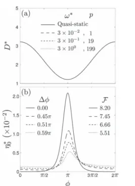
In Fig. 5, different angular frequencies u* are compared, whereas the time-average position D* and the oscillation amplitude A* are xed. As the probe trajectory is the same, whatever the frequency, so does the probe–liquid interaction term. Different values of p are considered in Fig. 5, according to the angular frequency u*, in order to compare oscillation cycles that start at the same time (except the quasi-static case), which in the presented case is t*¼ 2pp/u* ¼ 421.8. The surface apex evolution is symmetric with respect to f ¼ p for very low angular frequencies (typically u* # 10%6), corresponding to a
quasi-static situation. For larger values of u*, a symmetry breaking is induced by the gradually increasing role of the lm relaxation (drainage). In addition, the maximum deformation max(h0*) and the surface amplitude W* decrease, whereas the
lower lm position min(h0*) grows, for higher angular
frequencies u* (short oscillation periods). A more symmetric apex evolution provokes a shorter phase delay Df and a higher nesse F, which indicates that the curvature/interaction stage begins earlier and lasts longer during an oscillation cycle, and that the lm relaxation occurs faster in relation to the probe motion (low oscillation frequency u*). An asymmetric case denotes the opposite behaviour, as it can be clearly observed in Fig. 5.
5
Wavenumber analysis
5.1 Cutoff wavenumbers
In order to understand the behaviour of the liquid lm, one seeks the range of wavenumbers which are involved in this
Fig. 4 (a) Probe position D*, and (b) apex position h0*, as a function of phase f. All the curves were obtained for the same angular frequency u*¼ 3 + 10%1and probe lower position D* % A* ¼ 1:2121, but for different values of the probe oscillation amplitude A*.
Fig. 5 (a) Probe position D*, and (b) apex position h0*, as a function of phase f. All the curves were obtained for the same time-average probe position D* ¼ 2:2121 and probe oscillation amplitude A* ¼ 1, but for different values of the angular frequency u*.
phenomenon. The reciprocal of the modied capillary length [lCF*]%1works as the lower cutoff wavenumber of an innate
band-pass lter, since any distortion of the surface near r*¼ 0 tends naturally to propagate towards the modied capillary length. The upper cutoff, which is close to the wavenumber kmax*,
wherein the initial growth rate is maximum, is thus approximately: kmax*x2p & 1þ2e% e0 1eD ' ; (26) where: eD¼ 2p ffiffiffiffiffiffiffiffiffiffiffiffiffiffiffiffiffiffiffi ½D*'2% 1 q ; e0¼ eD &K1ðeDÞ K2ðeDÞ ' ; e1¼ eD ( &K1ðeDÞ K2ðeDÞ '2 % K0ðeDÞ K2ðeDÞ ) þ 2&K1ðeDÞ K2ðeDÞ ' : (27)
K0, K1and K2are zero, rst and second order modied Bessel
function of the second kind. The maximization procedure of the wavenumber distribution at t*¼ 0, which leads to nd kmax*, is
detailed in Appendix B. It is important to note that there is no relationship between kmax*and the other parameters appearing
in eqn (18), i.e. the modied capillary length lCF* and the
Hamaker number Ha. The wavenumber kmax*that corresponds
to the lower probe position D*¼ D* % A* operates as the upper cutoff of the innate lm band-pass lter. Furthermore, this particular value of kmax* has been employed as the cutoff
wavenumber in the numerical method.
The cutoff wavenumbers [lCF*]%1and kmax*have been
pre-sented in Fig. 2, proving the existence of a natural band-pass lter, which arises spontaneously from the physical and geometrical properties of the probe–lm system. In other words, the structures that are observed at the lm surface are always larger than [kmax*]%1but shorter than lCF*.
5.2 Wavenumber dynamics
Further understanding of the probe–lm coupling can be ach-ieved by assuming that D* [ x*h*, a small surface deformation compared to the separation distance, in eqn (12b). Aer applying the Hankel transform to the interaction potential, one nds Q *¼ %[k*]2Qs*, with Qs*given by:
Qs*ðk*; D*Þ ¼ K2 4 k* ffiffiffiffiffiffiffiffiffiffiffiffiffiffiffiffiffiffiffi ½D*'2% 1 q 5 ½D*'2% 1 : (28) The use of eqn (28) and a subsequent Fourier decomposition turns eqn (18) into a linear non-homogeneous ODE with analytical solution. This procedure, which is explained in-depth in Appendix C, yields the solution in the wavenumber domain:
N*¼pHa 4x* ( a0½1 % expð % n*t*Þ' þX N j¼1
8ajcos9ju*t* % 4j: % ~ajexp9 % n*t*:;
) ; (29) where ~ ajðk*Þ ¼ ajn* sj ; sjðk*Þ ¼ ffiffiffiffiffiffiffiffiffiffiffiffiffiffiffiffiffiffiffiffiffiffiffiffiffiffiffiffi ½ ju*'2þ ½n*'2 q ; 4jðk*Þ ¼ arctan 4ju* n* 5 : (30)
Eqn (29) provides an entire portrait of the wavenumber distribution dynamics and, as a consequence, the lm surface evolution, although its Hankel transform must be obtained numerically. Additionally, a matching wavenumber ku*
emerges from the comparison between n* and u*. Using the denition given in eqn (20), ku*is given by:
ku*¼ 1 ffiffiffi 2 p % % ½lCF*'%2þ ffiffiffiffiffiffiffiffiffiffiffiffiffiffiffiffiffiffiffiffiffiffiffiffiffiffiffiffiffiffiffi ½lCF*'%4þ 4u* q (1=2 : (31)
The wavenumber-dependent coefficients a0and aj, which are
dened in Appendix C and can only be computed numerically, together with the coefficients ˜ajand the phase 4j, are shown in
Fig. 6 as a function of the wavenumber k*, wherein two different behaviours are discerned in respect of ku*. For small
wave-numbers [lCF*]%1< k* < ku*, the a0coefficient dominates over
the others and a constant phase 4j¼ p/2 is found for any value
of j. In other words, as it can be discerned from eqn (29), the surface shape contribution, given by wavenumbers k* < ku*, is
not modied by the probe oscillation. Therefore, this wave-number range portrays the transitory behaviour of the lm surface, in the large time scale t*- [lCF*]4. As k* takes values
near the matching wavenumber ku*, the rst coefficients ajand
˜aj, obtained with small j values, gain importance with respect to
a0. The phase 4jdisplays the same trend for any j, diminishing
its value towards a zero phase as k* increases, and prematurely triggered for the large j terms. For large wavenumbers, ku*< k* <
kmax*, all the coefficients become as weighty as a0, and a
constant phase 4j ¼ 0 is recovered for any j. Therefore, as
deduced from eqn (29), the surface shape contribution dis-played by wavenumbers k* > ku*is completely driven by the
probe oscillation. Thence, this range of large wavenumbers describes the periodic response of the lm surface, in the short time scale t*- [u*]%1.
Briey, the lm surface shape is partially described by a prole that saturates exponentially (given for k* ˛ [(lCF*)%1,
ku*]), due to the gradual amassing of liquid below the probe.
This description is in agreement with the behaviour depicted in Fig. 2. In turn, along an oscillation cycle, the probe motion excites wavenumbers in the range k* ˛ [ku*, kmax*], which
provokes the surface oscillation around the saturation prole, spanning in the radial direction from the position beneath the probe to 15 times the probe radius. Since the time decay coef-cient n* is a function of the wavenumber k*, this probe excited wavenumber range, ku* < k* < kmax*, reaches a steady-state
earlier than the le-hand side wavenumber distribution, k* <
ku*.
It is important to note that for thin lms (small E* and, consequently, shorter lCF*) and higher frequencies u*, the
matching wavenumber ku*takes larger values. In this situation,
the range of wavenumbers excited by the probe is narrowed, which also provokes a reduction in the radial extent of the lm surface oscillation. The inverse effect should be produced for thick lms (large E* and lCF*) or lower frequencies u*.
Since the evolution of N * lies on the wavenumber-dependent coefficient n*, a complete steady-state surface oscillation is reached only when time is comparable with the reciprocal of the lower cutoff wavenumber, i.e. t* [ [lCF*]4. Thenceforth, the
stationary periodic regime is obtained when the exponential functions in eqn (29) are dismissed. For the case of a “slow” probe motion, which corresponds to a low frequency u* ( [lCF*]%4, the matching wavenumber becomes ku* z 0, and the
coefficients sjand the phases 4jreduce to sj¼ n* and 4j¼ 0.
This leads to the “slow” wavenumber distribution, which in the stationary state reduces to:
N*¼pHa½k*'
4
4x*n* Qs
*
ðk*; D*Þ: (32)
The liquid lm has enough time to recover its nearly at shape at the end of each oscillation cycle, which corresponds approximately to the static deformation obtained with the farther probe position D*¼ D* þ A*. The lm drainage occurs faster than the probe action, which inhibits the amassing of liquid and the increase of the lm surface deformation. Therefore, the lm oscillation process develops as a quasi-static phenomenon, revealing a surface shape that is equal to the static probe case for the same D*, at any instant of the oscilla-tion cycle. The proof of this fact is the behaviour of the apex deformation h0*during an oscillation, which is symmetric with
respect to f¼ p, as shown in Fig. 7.
In contrast, the probe motion is said to be “fast” when u* [ [kmax*]4, which yields sj¼ ju* and 4j¼ p/2. Since kmax*> lCF*,
therefore ku*- [u*]1/4, which implies that a0is dominant over
any aj. As a consequence, the “fast” wavenumber distribution
for the stationary state is given by:
N*¼pHaa0
4x* : (33)
In this situation, the liquid lm does not have sufficient time to react to the probe oscillation. During the transitory regime, the lm was not able to dissipate the energy injected at each cycle, which has been rather stored as an excess surface energy. Its amount is equivalent to the potential energy due to the liquid volume gathered near the probe position. Therefore, at the stationary state, the liquid surface remains with a “frozen-like” deformed shape, which is described by eqn (33). Since this expression only contains the constant term of the Fourier series of Qs*, the surface shape does not correspond to a deformation
prole generated by a static probe. Owing to the “fast” probe motion, the liquid lm does not have enough time to spread the excess liquid volume, from the surroundings of r*¼ 0 towards the outer zone, to recover its at prole, as it does for the quasi-static case. As it is shown in Fig. 7, the lm surface keeps the same sharp shape (around r*¼ 0) along the entire oscillation cycle, as well as constant apex position h0*and a deformation
extent that is shorter than lCF*.
Also in Fig. 7, the surface apex position is shown for an oscillating probe with a frequency of u* ¼ 3 + 10%1, corre-sponding to the intermediate frequency case shown in Fig. 5, which also occurs between the quasi-static and frozen-like behaviours. As it has already been mentioned, the apex evolu-tion is not symmetric with respect to f ¼ p because of the
Fig. 7 Stationary state apex surface position h0* as a function of phase f, in the stationary regime. Insets display the surface position h* as a function of the radial position r* for f ¼ 0 and f ¼ p. All the curves were obtained with D* ¼ 2:2121 and A* ¼ 1. The quasi-static behaviour corresponds to eqn (32), in which u* ( [lCF*]%4, whereas the frozen-like behaviour is given by eqn (33), in which u* [ [kmax*]4, and the intermediate steady-state case, u* ¼ 3 + 10%1, is yielded by eqn (29) with j ¼ 10 coefficients.
Fig. 6 (a) Coefficients and (b) phase of the solution given by eqn (29), for D* ¼ 2:2121, A* ¼ 1 and u* ¼ 3 + 10%1. The arrows indicate the terms corresponding to an increasing value of j.
alternating dominant role between lm drainage and probe– liquid interaction. In addition, as it can be discerned from a comparison between eqn (29) and (33), a lm surface, in the intermediate regime and the steady-state, oscillates around the frozen-like shape.
6
Critical oscillation parameters and
wetting transition
Fig. 8 shows the surface vertical position and the Fourier–Bessel coefficients Cmfor different probe lower positions, above and
below the value D*% A* ¼ Dmin*, at the instant of maximum
probe–liquid interaction f¼ p. For relatively large distances
D*% A* $ Dmin*, the lm surface shows a narrow prole, below
the probe position r* ˛ [0, 2], surrounded by a not deep annular crater. Even though the vertical position of the liquid surface increases at each cycle, it remains far away from the probe lower surface. In addition, the direct effect of the probe–liquid inter-action, represented by the large wavenumber side k* > ku*of the
Cmdistribution, quickly reaches a steady-state, opposite to the
small wavenumber side k* < ku*, which indicates the slow
diffusion of deformation energy towards larger radial positions, before attaining the stationary regime. On the other hand, for shorter separation distances D*% A*\Dmin*, the surface
prole can never reach a steady-state, because the liquid jumps-to-contact the probe. The probe–liquid interaction increases at each oscillation, provoking the amassing of liquid below the probe position. Thus, the lm surface exhibits progressively a more stretched prole, which becomes a vertical column of liquid at the last observable oscillation. At this last p cycle, at
which the p value decreases along with the lower probe position
D*% A*, the liquid touches the probe surface. Under these circumstances, the Cmdistribution of the last period p presents
a large wavenumber side k* > ku*, that is considerably
magni-ed with respect to the previous cycles, highlighting a signi-cant augmentation of the probe–liquid interaction, which cannot attain a stationary regime. As observed when comparing Fig. 8e and f, the probe wetting is characterized by a Cm
distri-bution of the same shape and magnitude in the wavenumber range k* > ku*. As a consequence, the same deformation below
the probe and a threshold intensity of the interaction are found, regardless of the number of cycles p before the jump-to-contact occurs. Nevertheless, the value of p indicates the periods that the system takes to attain this interaction frontier, due to the alternating attraction–relaxation stages. Therefore, a sequential transition from a stable surface oscillation regime with p / N, observed for distant lower probe positions D*% A* . Dmin*, to a
delayed wetting phenomenon with p > 0, for D*% A*\Dmin*,
and an instantaneous probe wetting event for p¼ 0, for closer values D*% A* ( Dmin*, is discerned.
In Fig. 9, the surface oscillation amplitude W*, the phase delay Df and the nesse F, already dened in Fig. 3 and eqn (25), are shown as a function of the number of oscillation cycles
p and for a probe oscillation amplitude A*¼ 1. For relatively large lower distances D*% A* $ Dmin*, a stationary state is
pursued, and thus W* and Df reach a saturation value aer the transient regime, consisting of several oscillation cycles p z 25, whereas F slowly converges towards a constant level. The nal stage of W*, Df and F becomes higher as D*% A* diminishes and approaches Dmin*. For slightly shorter distances
0:95Dmin*\D*% A*\Dmin*, aer the initial stage of the
Fig. 8 (a–c) Surface vertical position h* as a function of the radial position r* and (d–f) Fourier–Bessel coefficients Cmas a function of the wavenumber k*, for (a and d) D* % A* ¼ 1:009Dmin*, a non-wetting regime, (b and e)D*% A* ¼ 0:948Dmin*, a delayed wetting, and (c and f) D*% A* ¼ 0:945Dmin*, an instantaneous wetting phenomenon. All the curves were obtained for A*¼ 1 and u* ¼ 3 + 10%1, and they correspond to
transient regime, the growing rates of W*, Df and F tend to stabilize, although, they slowly continue to increase with faint slopes. For D*% A*\0:95Dmin*, the surface amplitude W* and
the nesse F curves look like inverse hyperbolic tangents. These quantities always increase, suffering from an important decrease in the growth rate during the rst cycles and reaching a minimum slope, and then, as the growth rate becomes unbounded again, W* and F are amplied until they diverge near a vertical asymptote. In turn, for these relatively small probe lower distances D*% A*, the phase delay Df increases strongly during the rst oscillations, which corresponds to an enhancement of the lm drainage effects and an important surface deformation along each oscillation cycle. Aerwards, as the cycles go by, Df calms down and its growth rate shows more gentle slopes, until it reaches a critical value Df - 0.58p, wherein it completely halts.
The divergence of W* and F, together with the halt of Df, indicates the wetting of the probe by the liquid lm depending on the lower probe position D*% A*. In Fig. 10, typical phase spaces, of the apex position h0*and the separation distance D*,
are shown for different values of D*% A*. For
D*% A* ¼ 1:01Dmin*, the liquid lm reaches the oscillatory
steady-state, a non-wetting behaviour, and thus a limit cycle attractor is observed in the phase space. This limit periodic
trajectory, of h0*as a function of D*, exhibits a “chistera” shape,
following a clockwise motion with smooth slopes around
D*¼ D* þ A* and a stepper path near D* ¼ D* % A*. This particular pattern is shown in Fig. 10a, up to p¼ 199 oscillation cycles. For D*% A* ¼ 0:95Dmin*, a delayed probe wetting of p¼
17 cycles is observed. In this case, although the apex displace-ment seems to reach a periodic orbit, its trajectory shis constantly towards greater values of h0*. As a consequence of
this gradual augmentation, the probe–liquid interaction becomes unbounded and the liquid rises to touch the probe, at the half-period of the p ¼ 17 cycle in Fig. 10b. Finally for
D*% A* ¼ 0:94Dmin*, the liquid lm touches the probe at the
rst oscillation cycle, as it is shown in Fig. 10c. Therefore, at the half-period of the rst cycle p¼ 0, the instant of maximum probe–liquid interaction, an instantaneous wetting process occurs aer a single barely curved trajectory of the liquid lm apex h0*. In brief, the liquid lm wets the probe for
D*% A*\Dmin*at a limit number of cycles p, which lessens as
the probe lower position D*% A* is shortened.
Fig. 9 (a) Surface oscillation amplitude W*, (b) phase delay Df and (c) finesse F as a function of the number of cycles p. All the curves were obtained for the same angular frequency u* ¼ 3 + 10%1and probe oscillation amplitude A* ¼ 1, but for different time-average probe positions in the range D* ˛½2:1383; 2:2121'. D* decreases in the sense of black arrows.
Fig. 10 Phase diagram of the apex position h0* and the separation distance D* of the three different behaviours: (a) non-wetting for
D*% A* ¼ 1:01Dmin*, showing a transient regime and approaching a
limit periodic orbit in the permanent state, (b) delayed wetting for
D*% A* ¼ 0:95Dmin*, showing a similar transient regime but diverging
from a possible limit orbit at the half-period of the p ¼ 17 cycle, and (c) instantaneous wetting for D* % A* ¼ 0:94Dmin*, showing a monotonic
trajectory that diverges immediately at p ¼ 0. Curves obtained with A*¼ 1 and u* ¼ 3 + 10%1.
7
AFM experimental consequences
The results presented in this theoretical study correspond to a typical AFM–lm system, consisting of a silicon probe oscil-lating near a liquid PDMS lm placed over a silicon wafer (substrate), with specic physical and geometrical properties and a single combination of dimensionless parameters (Ha, Bo,
ˆ
H, E*), which has been already given in Section 3.3. The effect of
these dimensionless numbers can be observed and analysed through their relationship with the merging length, time and wavenumber scales (see eqn (13) and (17) and Fig. 2): modied capillary length lCF¼ 2.2 + 10%7m, lm time scale s¼ 1.35 +
10%7s, transitory regime duration t- s[lCF/R]4¼ 3.2 + 10%2s
and lower cutoff wavenumber k¼ [lCF]%1¼ 4.5 + 106m%1. In
addition, we recall the static threshold Dmin, the separation
distance below which the liquid jumps-to-contact a static probe, which for the aforementioned parameters is Dmin ¼
1.2017+ 10%8m.
In contrast, different combinations of the probe oscillation parameters have been presented. The time-average probe posi-tion D and oscillaposi-tion amplitude A inuence directly the lm surface oscillation amplitude W, the probe wetting conditions and the corresponding limit of oscillation cycles p (see Fig. 4, 9 and 10). In addition, the impact of the probe oscillation frequency u lies on the wavenumber scales: upper cutoff wavenumber kmaxand matching wavenumber ku(see eqn (38)
and (31)). It is important to remember that these two quantities delimit the range of wavenumbers excited by the approach of the probe. Considering the aforementioned probe/lm/ substrate system and common dynamic NC-AFM tests, with frequencies in the range of 101 to 103kHz, oscillation ampli-tudes and probe–liquid separation distances restricted to the range of 1–25 nm, the probe activates a wavenumber range with lower ku ˛ [107, 108] m%1 and upper kmax ˛ [108, 109] m%1 boundaries.
This phenomenon can be analysed from an analogous viewpoint, performing a comparison between the two main time scales: the reciprocal of the angular frequency u%1, cor-responding to the experimental AFM time scale, and the char-acteristic lm time scale s, which also refers to the lm relaxation time.30 Therefore, the dimensionless angular
frequency u*¼ us is also identied as the Deborah number De
¼ ugE3/3mR,4
which herein characterizes the liquid lm response to a periodic AFM nano-probe periodic excitation. Large Deborah numbers De are obtained for liquids of high
viscosity m or relatively thin lms E, which correspond to large relaxation times s. This situation is also discerned when the lm is perturbed by a probe oscillating with a high frequency u [ [Rkmax]4/s, where kmax depends on the lower
probe position D% A. This high frequency case also yields a relatively large matching wavenumber, approximately kux R [us]1/4. In this large Deregime, the lm time scale s governs the
dynamics of the liquid surface. Since the surface h(r, t) evolves during the transient regime, nally reaching a steady-state h(r) independent of time t (see Fig. 7), a frozen-like behaviour of the lm is observed. Therefore, all the terms in eqn (11) become
constant over time. The viscous drainage restrains and slows down the lm dynamics, which coherently provokes a phase delay Df / p. As indicated by the observed nesse F / 2, the surface deformation is restrained to a span shorter than the modied capillary length lCF, and to relatively small vertical
displacements. The deformation energy is gathered below the probe position, generating a very narrow surface prole, due to the slow lm relaxation (drainage). Considering the probe– lm–substrate system analysed in this work, this frozen-like state should be observed for a probe oscillating around an average position D # 35 nm with an amplitude of A¼ 10 nm, only at frequencies above 10 MHz, which is only achieved with ultra-high frequency probes for high-speed AFM.
Small Deborah numbers De are found for liquids of low
viscosity m or relatively thick lms E, which yields short relax-ation times s. Equivalent similarity conditions are also gener-ated by low probe oscillation frequencies u( 1/s[lCF/R]4, which
for our specic thin lm corresponds to u( 3.1 + 101 s%1, leading to a matching wavenumber ku¼ 0. In this small De
regime, the AFM experimental time scale [u]%1determines the lm evolution, displaying a quasi-static behaviour. The viscous drainage occurs quickly and a full-period probe–liquid inter-action is observed, leading to a fast and full lm reinter-action, which corresponds to a phase delay Df / 0. At each instant, the surface attains the equilibrium shape of a static probe–liquid interaction phenomenon, with a maximum vertical displace-ment and a deformation extent that covers lCF. Therefore, the
drainage term in eqn (11) becomes negligible, and the probe– liquid interaction is only opposed by the curvature term throughout an oscillation cycle. This behaviour is validated by a large valued nesse F, pointing out that the deformation energy is spread over a large radial span, owing to a relatively rapid lm relaxation (drainage). For the parameters of the proposed probe–lm–substrate system, this regime is perceived for a probe oscillating with a frequency lower than 5 Hz, which is hardly considered as a dynamic AFM mode. Note that this frequency increases as the thickness of the lm is reduced. For instance, for a lm of 1 nm, the quasi-static threshold frequency is 5+ 105 Hz, which means that almost the entire NC-AFM
operation range presents a quasi-static behaviour. This last case must be considered for example when a thin layer of water is adsorbed over a silicon wafer.1,15
A comparison between the different De regimes,
corre-sponding to a thin lm of 10 nm, and several AFM modes, showing their frequency u range, is depicted in Fig. 11. The upper limit of the quasi-static behaviour, which is xed for a given lm thickness, also denes the limit of force spectroscopy tests, whereas the lower boundary of the frozen-like behaviour moves according to the probe lower position. In the presented diagram, normal NC-AFM experiments occur in the transition zone, above the quasi-static boundary, which indicates that the probe oscillation provokes a signicant surface oscillation amplitude and a transmission of surface energy to a large radial extent, but not as important as for the quasi-static case. The frozen-like boundary is located within the higher frequency range of high-speed NC-AFM experiments, implying surface proles with small surface oscillation amplitudes and
restrained radial spans, under these conditions. Although an equivalent diagram can be obtained for a lm of different thickness, a particular interpretation of the AFM modes should be done due to the thickness-dependence of De, s and lCF. For
instance, considering a lm with a thickness of 1 nm, a large range of normal NC-AFM experiments may be comprised in the quasi-static regime. On the other hand, the quasi-static state is never observed for NC-AFM tests over a lm of 100 nm, because the frequency needed to reach this situation becomes ve orders of magnitude smaller than that for the 10 nm lm case. In Fig. 12, for a xed oscillation amplitude A*¼ 1, the limit number of oscillations before wetting p is shown as a function of
D*% A* % Dmin*the difference between the lower probe position
and the static minimum separation distance, also corresponding to the threshold jump-to-contact distance of a quasi-static situ-ation. The trend for an intermediate angular frequency u*¼ 3 + 10%1, which is located in the intermediate Deborah regime
[lCF*]%4< De< [kmax*]4, is shown in Fig. 12. The instantaneous
probe wetting occurs for D*% A*\Dmin*% 0:066, whereas a
delayed wetting behaviour is observed within the zone %0:066\D* % A* % Dmin*\% 0:057, and the oscillating
steady-state without wetting takes place for D*% A*\Dmin*% 0:057.
These three situations, which correspond to previously mentioned behaviours (see Fig. 10), are connected by a mono-tonically increasing dependency of p on D*% A* % Dmin*.
Inter-estingly, the non-wetting transition does not take place at
D*% A* ¼ Dmin*, the jump-to-contact threshold distance for a
static probe. In addition, the wetting transition for the two asymptotic frequency cases is also depicted in Fig. 12, for A*¼ 1. The right-hand side inlet in Fig. 12 corresponds to a small Deborah regime De( [lCF*]%4(quasi-static lm behaviour), in
which wetting may occur instantaneously for D*% A*\Dmin*,
following the same trend as the phase diagram in Fig. 10c with
p¼ 0. Under these conditions, an oscillating steady-state should always be observed for D*% A* $ Dmin*, equivalent to the
peri-odic trajectory shown in Fig. 10a. A delayed wetting event can
never occur for the quasi-static situation, and a straightforward transition from wetting to non-wetting is observed, displayed as a vertical asymptote overlapping the abscissa D*% A* % Dmin*¼ 0
in the right side inlet in Fig. 12. Dynamic NC-AFM experiments executed in this small Deregime are restricted to large separation
distances D% A > Dmin, which reduces signicantly the probe
sensitivity, in order to inhibit the probe wetting. On the other hand, the large Deborah regime De[[kmax*]4(frozen-like lm
behaviour) is displayed in the le-hand side inlet of Fig. 12. In this case, wetting is reprieved to shorter separation distances and a vertical asymptote placed at D*% A* % Dmin*¼ %0:153
indi-cates the wetting transition. This threshold distance has been
Fig. 11 AFM modes and liquid film behaviour depending on the Deborah number De. The boundaries for the quasi-static and frozen-like behaviour were placed according to their values for a film thickness of 10 nm and a lower probe position 1\D* % A*\3:5. Arrows (red) indicate the impact of decreasing the parameters: film thickness E* and the lower probe position D* % A*.
Fig. 12 Number of oscillation cycles p before wetting as a function of the difference between the lower probe position D* % A* and the static minimum separation distance Dmin*, obtained with A*¼ 1 and u* ¼ 3 + 10%1, within an intermediate Deborah regime [lCF*]%4< De< [kmax*]4. The quasi-static and frozen-like trends, including their wetting thresholds, are also depicted.
obtained by solving D*% A* ¼ x*h0*þ 1, with the use of eqn
(33). Therefore, when dynamic NC-AFM experiments are per-formed in this large Deregime, the liquid lm surface can be
scanned at shorter probe–liquid separation distances D% A <
Dmin, which increases the apparatus resolution without the risk
of wetting the probe or engendering a signicant surface deformation.
When performing NC-AFM experiments over liquids, one must prevent the sample damage and the probe wetting. The employment of a high oscillation frequency (large De regime)
allows “freezing” of the dynamic response of the liquid lm, which generates the following advantages:
(1) The probe–liquid separation distance can be shortened, increasing the AFM sensitivity and preserving the sample physical integrity. In the presented case, this distance, which corresponds to the probe lower position D*% A*, can be shortened by around 1.5 nm (see Fig. 12), around 13% of the static threshold separation distance11D
min.
(2) The amplitude of the liquid surface oscillation is small, thus the effect of its displacement over the measured topog-raphy is reduced. The maximum deformation of the surface is reduced up to 86%, from the quasi-static to the frozen-like regime (see Fig. 7).
(3) The surface oscillation is restrained and, as a conse-quence, the noise in the AFM signal is also diminished.
Since the probe–liquid separation distance is sometimes hard to control precisely in experiments, high oscillation frequencies contribute to performing successful measurements by creating a margin of the probe lower position. In addition, more accurate NC-AFM data can be retrieved by increasing the probe frequency, even if the large De regime is not always
attainable.
8
Conclusions
The dynamic response of a liquid lm due to its interaction with an oscillating nano-probe was studied by means of numerical simulations. Our analysis yielded the wavenumber scales, that limit the range excited by the probe at each oscillation cycle and that corresponding to the natural lm relaxation. The time scales which describe the transitory regime duration and the lm relaxation were determined, as well as the phase duration along an oscillation cycle for the governing deformation mechanisms. The effects of the time-average probe position, the probe oscillation amplitude and frequency were analysed. For large separation distances, a theoretical solution in the wave-number domain was obtained, which completely describes the dynamics of the lm surface. Moreover, asymptotic behaviours for the probe oscillation frequency were derived from the solution. A quasi-static deformation regime is observed for low oscillation frequencies, whereas a frozen-like behaviour is found for high frequencies. For short separation distances, the solution provided evidence of critical combinations of oscilla-tion parameters (time-average position, amplitude and frequency) that lead to prove wetting. Therefore, an educated selection of the oscillation parameters can be made based on
our results, depending on the experimental objectives, instead of nding them heuristically.
It is important to notice that the present analysis does not include the effect of thermal agitation. Under this premise, our work should be considered as a rst order approach, which yields the average behaviour of a liquid lm interacting with an oscillating probe. A posteriori and extensive analysis, including higher order corrections (which should certainly scale with kBT),
as it has been recently done for a static probe–bulk liquid interaction,35 must be taken into account in order to obtain
more precise picture of the lm interface.
The surface lm dynamics, exposed in this paper, may be useful to understand liquid properties and their behaviour at the micro- and nanoscopic scales. Furthermore, it has been proven that the dynamic NC-AFM mode provides a non-intru-sive tool to scan liquid samples, when a good choice of experi-mental parameters (frequency, free and set-point amplitude) is made. We expect that this work will lead to a quantitative understanding of the AFM imaging of so samples, mainly in the recovery of unspoilt sample topographies. Additionally, the introduced ideas should also be applied to analyse AFM experimental results when a thin lm of water covers the sample, as it is usually observed under uncontrolled humidity conditions. The importance of quantifying the effect of the adsorbed thin layer has been emphasised,15 because surface
deformation and capillary effects may lead to false interpreta-tions and to obtain inaccurate topographies.
Appendix
(A) Hankel transform and inverse transform denitions The Hankel transform of order zero of a function f, dened in the spatial r* and temporal t* domains, is dened by:
gðk*; t*Þ ¼ ℍ0f f ðr*; t*Þg ¼ 2p ðN 0 fðr*; t*ÞJ0ðk*r*Þr*dr*; (34)
whereas the inverse transform of a function g, dened in the angular wavenumber k*¼ Rk and time t* ¼ t/s domains, is given by: fðr*; t*Þ ¼ ℍ0%1fgðk*; t*Þg ¼ 1 2p ðN 0 gðk*; t*ÞJ0ðk*r*Þk*dk*; (35)
where J0is the zero-order Bessel function of the rst kind.
(B) Upper wavenumber cutoff
At the rst stages of the phenomenon, the upper cutoff kmax*
corresponds to the wavenumber at which the growth rate is maximum. At t*¼ 0, the lm free surface is at h* ¼ 0 and, as a consequence, its related wavenumber distribution is N *¼ 0. Nevertheless, the growth rate vN *=vt* is not null at this stage. If one applies: v vk* &vN * vt* ' ¼ 0 with N * ¼vN* vk*¼ 0 (36)