HAL Id: hal-00732995
https://hal.archives-ouvertes.fr/hal-00732995
Submitted on 17 Sep 2012
HAL is a multi-disciplinary open access
archive for the deposit and dissemination of
sci-entific research documents, whether they are
pub-lished or not. The documents may come from
teaching and research institutions in France or
abroad, or from public or private research centers.
L’archive ouverte pluridisciplinaire HAL, est
destinée au dépôt et à la diffusion de documents
scientifiques de niveau recherche, publiés ou non,
émanant des établissements d’enseignement et de
recherche français ou étrangers, des laboratoires
publics ou privés.
UWB channel modeling for objects evolving in impulsive
environnements
Nourddine Azzaoui, Laurent Clavier
To cite this version:
Nourddine Azzaoui, Laurent Clavier. UWB channel modeling for objects evolving in impulsive
en-vironnements. Wireless Communications and Networking Conference Workshops (WCNCW), 2012
IEEE, 2012, France. pp.191 - 195, �10.1109/GLOCOMW.2010.5700305�. �hal-00732995�
UWB channel modeling for objects evolving in
impulsive environnements
Nourddine Azzaoui and Laurent Clavier, Member, IEEE
Abstract—We consider channel modeling issues in the context where communicating objects are evolving in impulsive environ-ments. It was shown recently that α-stable random processes are attractive solution for representing the ultra wide band communication channel in relatively large spatial areas. In this paper, we consider the α-stable channel modeling in an evolutionary context where the model features depend on spatial locations. We introduce a methodological approach consisting of two parametric and non parametric components: the latter can be seen as black box model to describe the spatial evolution and it can be learned from historical observations of the transfer func-tion. The other component concerns the frequency dependence and has an auto-regressive structure.
INTRODUCTION
One important difficulty of statistical channel modeling (especially when ultra wide band (UWB) is considered) resides in its ability to represent the time and environment evolutions. This channel variability is obvious when it comes to model mobiles and rapidly changing environments. In order to make realistic simulations, it is necessary to adapt the existing models to such situations. Indeed, statistical models, even those taking into account rare events (α-stable models), are not sufficient to describe the complexity of the channel behavior in all circumstances. Another challenge for developing real world applications is the fact that the specification of a such model needs a large measurement campaign and usually takes a lot of time to estimate the model parameters. For the next generation communication systems, (as WSN, inter vehicles, ...), time evolution can be slow or fast and nodes will change their position and interact with different communication in-frastructures. They must be able to learn their environments autonomously, especially channel models of the medium in which they evolve. Due to the models complexity and possible fast evolution, this task is quasi impossible for the end user, especially low complexity sensor nodes.
The idea of this work is to give a general model that can adapt to the rapid change of the environment and learned from a limited number of measurements. For this purpose our proposed model must, from one hand, describe the space dependence of the channel transfer function and, on the other hand, the model variation with frequency. From this last point of view many works described this frequency dependence as
Nourddine Azzaoui is with the Mathematics Laboratory UMR-CNRS 6620 from of Blaise Pascal university, Aubi`ere (France).
Laurent Clavier is with IEMN (Institute of Electronics, Microelectronics and Nanotechnology, UMR CNRS 8520), IRCICA (Research Institute on software and hardware components of the future for information and com-munication, FR CNRS 3024) and TELECOM Institute, TELECOM Lille 1, Lille, France. This work was supported by the ERDF (European Regional Development Fund) and by the Nord-Pas-De-Calais Region (France).
parametric model: we cite for instance Ghassemzadeh [1] who uses a second-order autoregressive model AR(2) for frequency response generation of the UWB indoor channel. The work in this paper is an on going contribution, it presents the theory behind the model and solutions for space and frequency channel evolution in section I and some mathematical tools to estimate the parameters (section II) and validate the model (section III). Further investigations is needed to validate this approach. We also assume that the channel is accurately represented by an α-stable model as we proposed in [2].
I. THE EVOLUTIONARY CHANNEL MODEL
The main idea of the evolutionary model comes from the fact that transfer functions measured at two contiguous places will be strongly dependent; it will be weakly dependent when the distance increases between two measurements. For
the mathematical formulation let us denote Hx the transfer
function at a position x. We postulate that the dependence will have a memory of length p. This space dependence can be formulated using conditional expectations as follows:
Hx+1 = f (Hx, . . . , Hx−p) + Υ, (1)
where f is an unknown function not depending on the location
and Υ = Hx+1− E (Hx+1| Hx, . . . , Hx−p). Equation (1) can
be seen as a black-box model which does not support any a
priori about the environment. One of its main advantages is
the fact that it can be learned (estimated non parametrically using kernel techniques) from historical observations collected by a given node. In order to understand the frequency depen-dence we present the model for observed transfer functions at
w1, . . . , wn, as the following: pos p Hp+1(w1) = f (Hp(w1), . . . , H1(w1)) + Υp(w1) .. . ... Hp+1(wn) = f (Hp(wn), . . . , H1(wn)) + Υp(wn) .. . ... ... pos x Hx+1(w1) = f (Hx(w1), . . . , Hx−p(w1)) + Υx(w1) .. . ... Hx+1(wn) = f (Hx(wn), , . . . , Hx−p(wn)) + Υx(wn)
Index p denotes the length of the dependence, consequently, the number of samples that nodes has to store in order to start
its estimation. For different positions x and x0, we suppose
that vectors Υx and Υx0 are pairwise independent. Since the
function f has captured all the intrinsic spatial influence, it makes more sense to suppose that Υ depends only on
frequencies. Inspired from works in [1], we suppose that for a fixed position, the internal frequency dependence of Υ may be described by an autoregressive scheme.
Υx(wi) = q
X
k=1
θkΥx(wi−k) + εx,i (2)
In order to take into account the impulsive nature and the
α-stable model [2], we suppose that errors εx,i’s are i.i.d.
symmetric α-stable white noises.
The main difficulty in the black-box model (1) arises when we try to estimate the non parametric function f which will be seriously affected when p becomes large; this is known as the curse of dimensionality. In order to overcome such an
in-convenience we will suppose that, instead of (Hx, . . . , Hx−p),
the transfer function Hx+1 depends on a linear combination
of this vector. This reduce f to a real function and hence its estimation is facilitated. This will lead to the following:
Hx+1(wi) = f ( p X k=0 ηkHx−k(ωi)) + q X k=1 θkΥx(wi−k) + εx,i (3)
To resume, f represents the space dependence, the coefficient
θk the frequency linear dependence and εx,ithe unpredictable
variations. This model is very general and will allow the use of powerful mathematical tools known in literature as semi parametric single index partially linear model. They have been largely studied in literature we cite among others [3], [4], [5], [6]... For compatibility with the semi-parametric formalism we rearrange the observed transfer functions as follows: we begin by taking N = nm where n is the number of positions and m is the number of observed frequencies. For every x = 1, . . . , n − 1, for every i = 1, . . . , m we take s = (x − 1)m + i and we denote: Ys= Hx+1(wi), Us= [Hx(wi), . . . , Hx−p(wi)]†, Vs= [Υx(wi−1), . . . , Υx(wi−q) ]†, Xs= [Us†, V † s] †, εs= εx,i
where † states for matrix transpose. This will lead to the conventional semi parametric single index model notations:
Ys= Xs†θ + f (X †
sη) + εs (4)
where θ = (0p+1, θ1, . . . , θq) and η = (η0, . . . , ηp, 0q)
and 0p is zeroes vector in Rp.
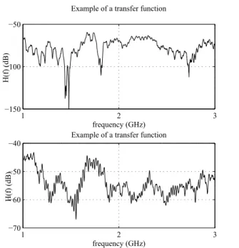
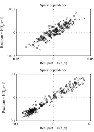
Motivation for using (4) for independent data analysis can be found in [5], [6], [7]. Many indications suggest the use of semi-parametric models (4); for example two transfer functions are presented in Fig. 1. Figures Fig. 2 and Fig. 3 illustrate the space and frequency dependence. The autoregres-sive scheme was also noticed in [1] and confort our proposal.
II. STATISTICAL ESTIMATION AND MODEL SPECIFICATION
FOR THE EVOLUTIONARY MODEL
In this paper, we will address the estimation problem in the α-stable case and introduce consistent estimators of unknown
1 2 3 −150 −100 −50 frequency (GHz) H(f) (dB)
Example of a transfer function
1 2 3 −70 −60 −50 −40 frequency (GHz) H(f) (dB)
Example of a transfer function
Fig. 1. Examples of measured transfer functions between 57-59 GHz and down converted between 1-3 GHz at two different locations. More details on the measurement setup can be found in [2], [8]
. −0.05 0 0.05 −0.05 0 0.05 Real part − H(f,x) Real part − H(f+ ∆ f ,x) Frequency dependence (∆f=5MHz) −0.1 0 0.1 −0.1 0 0.1 Real part − H(f,x) Real part − H(f+ ∆ f ,x) Frequency dependence (∆f=5MHz)
Fig. 2. Spatial dependence structure in observed transfer functions. The distance between x and x+1 is 2.5mm. Two different locations in the computer room are considered.
−0.05 0 0.05 −0.05 0 0.05 Real part − H(f0,x) Real part − H(f 0 ,x−1) Space dependence −0.1 0 0.1 −0.1 0 0.1 Real part − H(f0,x) Real part − H(f 0 ,x−1) Space dependence
Fig. 3. Frequency dependence structure in observed transfer functions. The frequency step is 5 MHz.
model (4) features; the mode of convergence and the quality of the estimators will be detailed in further works.
A. Estimation in semi parametric single index models Consider a semi-parametric single-index model of the form:
Ys= Xs†θ + f (X
†
sη) + εs, s = 1, 2, . . . N, (5)
where both θ and η are vectors of unknown parameters. The real function f (·) is unknown defined on R and is supposed
to be twice differentiable. The random variables {εs} are a
sequence of errors with E[εs | Xs] = 0. A huge amount of
works about such models have been introduced in literature especially when the errors are random variables with finite second order moments; for more details see for instance [5] and [7]. However no works have been done in the case of infinite variance errors. In this paper we suppose that the
εs’s are i.i.d. α-stable centered variables with a fixed scale
parameter σ.
In order to estimate the unknown parameters η, θ and the function f involved in (5), we introduce the following notation:
f1η(u) = E[Ys| Xs†η = u], (6)
f2η(u) = E[Xs | X †
sη = u], (7)
This decomposition is inspired from the conditional
decom-position f (u) = E[Ys− Xs†θ | Xs†η = u] which leads easily
to the formula:
f (u) = f1η(u) − (f2η(u))†θ (8)
Let K be a kernel function i.e. a non negative even probability
density (for example the gaussian kernel K(x) = √1
2πe −x2
2 ).
From the conditional expectation given in (6) we propose a kernel estimation inspired from the Nadarya-Watson
estima-tion techniques. We first estimate f1η(·) by:
ˆf 1η(u) = N X s=1 Kh(X † sη − u)Ys N X s=1 Kh(Xs†η − u)
where Kh(·) = K(h·) and h is a bandwidth parameter.
Similarly we estimate the function f2η(·) by:
ˆ f2η(u) = N X s=1 Kh(Xs†η − u)Xs N X s=1 Kh(X † sη − u)
For a complete estimation of the function f we will need an estimate of the parameters η and θ. For this purpose we use the following notations:
Ysη= Ys− ˆf1η(X † sη), Xsη= Xs− ˆf2η(X † sη),
Let us consider the least-squares sum :
SN(θ, η; h) = N X s=1 (Ysη− X † sηθ) 2
The estimation idea consist in minimizing SN(θ, η, h) over
(θ, η, h). We first remark that, for a fixed (η, h), the least squares estimator of θ can be deduced using classical linear regression techniques, it is given by:
ˆ θ(η, h) = N X s=1 XsηX † sη !+ N X s=1 XsηYsη, (9)
where ( . )+ denotes matrix pseudo-inverse. We then estimate
(η, h) by (ˆη, ˆh) through minimizing, ˆ SN(η, h) = N X s=1 (Ysη− X † sηθ(η, h))ˆ 2 (10)
Inspired from the equation (8), we propose the nonparametric
estimator of f (·) by using estimates of f1η and f2η:
ˆ
f (u) = ˆf1ˆη(u) − (ˆf2ˆη(u)) †ˆ
θ(ˆη, ˆh). (11)
On the other hand, when the errors scale parameter σ is unknown, it can be estimated using the fractional lower moments technique as follows:
ˆ σ = Cα(ρ) 1 N N X s=1 Ysˆη− X † sˆηθ(ˆˆ η, ˆh) ρ! 1 ρ (12)
for every 1 < ρ < α and Cα(ρ) is an universal constant
depending only on α and ρ, it is given by:
Cα(ρ) = α√π Γ(−ρ2 ) 2ρ+1Γ(1+ρ 2 ) Γ( −ρ α) !1ρ
The mode of convergence and the consistency of these esti-mators was studied in the second order case, the reader find a detailed overview in literature; see for instance [7]. In this last work a central limit theorem type result was established for all estimators. We believe that similar results may be proven for the α-stable process and will be similar to the generalized central limit theorem context.
III. MODELS ADEQUACY AND HYPOTHESIS TESTING
In this section we present statistical techniques to test the ad-equacy of semi parametric models of type (4). Recently, semi-parametric approach has been used for model specification tests in the case of finite variance processes. We will proceed by analogy to second order works, we focus on partially linear or single-index scheme against a general non-parametric form. We concentrate on parametric specification testing of the
conditional mean function defined for u ∈ Rp+q+1 by:
m(u) = E[Ys| Xs= u)]
A. Testing for single-index regression
In this subsection we focus on the particular case of (4) without the linear regression component. The test purpose is to see if transfer functions evolutions can be reduced to the space
evolution, not considering the frequency dependency (H0).
Somehow it can be seen as a test for spatial stationarity of transfer functions. We thus look at testing the null hypothesis of single index modeling against a class of non parametric functions:
(H0) : m(x) = f (x†η),
(H1) : m(x) = f (x†η) + ∆(x) for all x ∈ Rp+1,
where f (·) is an unknown function on R, η is a vector of unknown parameters and ∆ is any regular function defined
on Rp+1. Under the null hypothesis (H0) we have given
techniques to estimate η in section II. In the single index particular case the estimate of f (·) will be simplified and is given by: ˆ f (Xs†η) = N X t=1 YtK( (Xs− Xt)†η h ) N X u=1 K((Xs− Xu) † η h ) ,
with K(·) being a kernel function defined on R. Consequently, from (10) the parameter η is then estimated by minimizing:
ˆ η = arg min (η,h) N X s=1 (Ys− ˆf (X † sη))2
As we have supposed that the errors εs’s are α-stable i.i.d.
cen-tered random variables, then by the generalized central limit theorem it is more convenient to approximate the estimated
errors ˆYs = Ys− ˆf (Xs†η) by a centered symmetric α-stableˆ
distribution with estimated scale parameter ˆσ:
ˆ σ = Cα(ρ) 1 N N X s=1 ˆ Ys ρ! 1 ρ
By analogy with the second order case and for compatibility with infinite variance we suggest the test statistic:
L = N X s=1 | ˆYs| ˆ σ
Many improvements are still needed in the case of stable variables, including the asymptotic distribution and robustness of the statistic L. For the hypotheses testing in the case of second order semi parametric models one can find a rich literature in [9], [4], [10] and references within.
B. Testing for partially linear single-index model
It is a natural extension of the single index model to situa-tions where the linear regression component may be suitable for modeling the inherent studied phenomenon. The following test evaluates if the dependency on space and frequency is
sufficient (H0) or if it would be more accurate to take some
more phenomena into account, for instance some non linear dependency in frequency.
(H0) : m(x) = x†θ + f (x†η)
(H1) : m(x) = x†θ + f (x†η) + ∆(x),
for all x ∈ Rp+q+1. This test problem has been studied for the
second order case by [5], [6]. With the same reasoning as in the single index model and by using the estimation techniques
under the hypothesis (H0) presented in section II, we propose
the test statistic:
L = N X s=1 | cYs| ˆ σ
where cYs= Ys− Xs†θ − ˆˆ f (Xs†η), the quantities ˆˆ θ, ˆη, ˆf (·) and
ˆ
σ are respectively the consistent estimators given in (9), (10), (11) and (12). One of the main issues to evaluate the models compatibility is to examine the power and the size tests :
α = P(L > lα | such that H0”holds” )
β = P(L > lα | such that H1”holds” )
where lαwill be tabulated from the distribution of L. It should
be noted that the estimator presented here must be extensively studied for asymptotic properties and robustness.
CONCLUSION AND PERSPECTIVES
In this paper we have introduced a methodological approach that adapts semi-parametric techniques to the context of spatial ultra wide band channel modeling. Our approach may be seen as a general-purpose framework for the modeling of the spatial evolution of the channel transfer functions described by an α-stable random process. Extensive simulations on real data must be performed to evaluate the adequacy of the proposed model in the context of indoor and outdoor configurations and this paper only presents the general framework.
REFERENCES
[1] S. Ghassemzadeh, R. Jana, C. Rice, W. Turin, and V. Tarokh, “Measure-ment and modeling of an ultra-wide bandwidth indoor channel,” IEEE Transactions on Communications, vol. 52, no. 10, pp. 1786–1796, 2004. [2] N. Azzaoui and L. Clavier, “Statistical channel model based on α-stable random processes and application to the 60 GHz ultra wide band channel,” IEEE Transactions on Communications, vol. 58, no. 5, pp. 1457–1467, 2010.
[3] R. Carroll, J. Fan, I. Gijbels, and M. Wand, “Generalized partially linear single-index models,” Journal of the American Statistical Association, vol. 92, no. 438, pp. 477–489, 1997.
[4] J. Gao and H. Liang, “Statistical inference in single-index and partially nonlinear models,” Annals of the Institute of Statistical Mathematics, vol. 49, no. 3, pp. 493–517, 1997.
[5] Y. Xia, H. Tong, and W. Li, “On extended partially linear single-index models,” Biometrika, vol. 86, no. 4, p. 831, 1999.
[6] Y. Xia, W. Li, H. Tong, and D. Zhang, “A goodness-of-fit test for single-index models,” Statistica Sinica, vol. 14, no. 1, pp. 1–27, 2004. [7] J. Gao, Nonlinear Time Series Semiparametric and Nonparametric
Methods. Chapman & Hall/CRC, 2007.
[8] M. Fryziel, C. Loyez, L. Clavier, and R. N., “Path loss model of the 60 GHz radio channel,” Microwave and optical technology letters, vol. 34, no. 3, pp. 158–162, Aug. 2002.
[9] Y. Fan and Q. Li, “Consistent model specification tests: omitted variables and semiparametric functional forms,” Econometrica: Journal of the Econometric Society, vol. 64, no. 4, pp. 865–890, 1996.
[10] W. Stute and L. Zhu, “Nonparametric checks for single-index models,” Annals of Statistics, vol. 33, no. 3, pp. 1048–1083, 2005.