Algorithms for Robust Autonomous Navigation
in Human Environments
by
Michael F. Everett
S.B., Massachusetts Institute of Technology (2015)
S.M., Massachusetts Institute of Technology (2017)
Submitted to the Department of Mechanical Engineering
in partial fulfillment of the requirements for the degree of
Doctor of Philosophy
at the
MASSACHUSETTS INSTITUTE OF TECHNOLOGY
September 2020
© Massachusetts Institute of Technology 2020. All rights reserved.
Author . . . .
Department of Mechanical Engineering
June 22, 2020
Certified by. . . .
Jonathan P. How
R. C. Maclaurin Professor of Aeronautics and Astronautics
Thesis Supervisor
Certified by. . . .
Alberto Rodriguez
Associate Professor of Mechanical Engineering
Thesis Supervisor
Certified by. . . .
John Leonard
Samuel C. Collins Professor of Mechanical and Ocean Engineering
Thesis Committee Chair
Accepted by . . . .
Nicolas Hadjiconstantinou
Graduate Officer, Department of Mechanical Engineering
Algorithms for Robust Autonomous Navigation
in Human Environments
by
Michael F. Everett
Submitted to the Department of Mechanical Engineering on June 22, 2020, in partial fulfillment of the
requirements for the degree of Doctor of Philosophy
Abstract
Today’s robots are designed for humans, but are rarely deployed among humans. This thesis addresses problems of perception, planning, and safety that arise when deploying a mobile robot in human environments. A first key challenge is that of quickly navigating to a human-specified goal – one with known semantic type, but unknown coordinate – in a previously unseen world. This thesis formulates the con-textual scene understanding problem as an image translation problem, by learning to estimate the planning cost-to-go from aerial images of similar environments. The proposed perception algorithm is united with a motion planner to reduce the amount of exploration time before finding the goal. In dynamic human environments, pedes-trians also present several important technical challenges for the motion planning system. This thesis contributes a deep reinforcement learning-based (RL) formula-tion of the multiagent collision avoidance problem, with relaxed assumpformula-tions on the behavior model and number of agents in the environment. Benefits include strong performance among many nearby agents and the ability to accomplish long-term autonomy in pedestrian-rich environments. These and many other state-of-the-art robotics systems rely on Deep Neural Networks for perception and planning. How-ever, blindly applying deep learning in safety-critical domains, such as those involving humans, remains dangerous without formal guarantees on robustness. For example, small perturbations to sensor inputs are often enough to change network-based deci-sions. This thesis contributes an RL framework that is certified robust to uncertainties in the observation space.
Thesis Supervisor: Jonathan P. How
Title: R. C. Maclaurin Professor of Aeronautics and Astronautics Thesis Supervisor: Alberto Rodriguez
Title: Associate Professor of Mechanical Engineering Thesis Committee Chair: John Leonard
Acknowledgments
I did not plan to be at MIT for so long and definitely did not plan to do a PhD. There are a lot of people to thank for making it a great experience.
First, I want to thank my advisor, Professor Jonathan How, for his support, motivation, and mentorship throughout graduate school. He sets the bar high and invests a ton of his own time to help his students be successful.
Thank you to the thesis committee: Professor John Leonard and Professor Alberto Rodriguez have helped me to think critically about where my work fits into the field and how it ties together, and they have also given extensive, invaluable advice about how to begin my career after the PhD.
The Aerospace Controls Laboratory (ACL) has been an awesome place to learn to become a researcher. Although I study neither Aerospace nor Controls, the wide range of people and projects in the lab have helped me learn a little about so many different topics. Thank you in particular to Drs. Steven Chen, Justin Miller, Brett Lopez, Shayegan Omidshafiei, and Kasra Khosoussi who taught and inspired me more than they realize. The pursuit of international cuisine while traveling with Björn Lütjens and Samir Wadhwania (inspired by Dong-Ki Kim) was also quite memorable. Dr. Shih-Yuan Liu and Parker Lusk have been guiding voices about writing code the right way, even if it is not the fastest way that day (along with other great advice). Thank you to Building 41 for providing some perspective on Building 31.
Thank you to Ford Motor Company, and in particular, ACL alumnus Dr. Justin Miller and Dr. Jianbo Lu: they have supported my research through thoughtful discussions during monthly telecons and campus visits over the years, as well as financially. It has been motivating to have a group of collaborators that are also working hard to see these technologies come to life.
Thank you to Meghan Torrence for helping me realize I should do a PhD and for making it a lot more fun.
Finally, I thank my family members for their support: Mom (’79 SB, ’81 SM), Dad (’76 SB, ’91 PhD), Tim, Katie (’12 SB, ’13 MEng), and Patrick (’17 SB).
Contents
1 Introduction 19
1.1 Overview . . . 19
1.2 Problem Statement . . . 20
1.2.1 Planning Without a Known Goal Coordinate or Prior Map . . 21
1.2.2 Planning Among Dynamic, Decision-Making Obstacles, such as Pedestrians . . . 21
1.2.3 Deep RL with Adversarial Sensor Uncertainty . . . 21
1.3 Technical Contributions and Thesis Structure . . . 22
1.3.1 Contribution 1: Planning Beyond the Sensing Horizon Using a Learned Context . . . 22
1.3.2 Contribution 2: Collision Avoidance in Pedestrian-Rich Envi-ronments with Deep Reinforcement Learning . . . 22
1.3.3 Contribution 3: Certified Adversarial Robustness for Deep Re-inforcement Learning . . . 23
1.3.4 Contribution 4: Demonstrations in Simulation & on Multiple Robotic Platforms . . . 23 1.4 Thesis Structure . . . 23 2 Preliminaries 25 2.1 Supervised Learning . . . 25 2.1.1 Deep Learning . . . 26 2.2 Reinforcement Learning . . . 26
2.2.2 Learning a Policy . . . 27
2.2.3 Deep Reinforcement Learning . . . 28
2.3 Summary . . . 28
3 Planning Beyond the Sensing Horizon Using a Learned Context 29 3.1 Introduction . . . 29 3.2 Background . . . 31 3.2.1 Problem Statement . . . 31 3.2.2 Related Work . . . 33 3.3 Approach . . . 36 3.3.1 Training Data . . . 36
3.3.2 Offline Training: Image-to-Image Translation Model . . . 38
3.3.3 Online Mapping: Semantic SLAM . . . 38
3.3.4 Online Planning: Deep Cost-to-Go . . . 39
3.4 Results . . . 41
3.4.1 Model Evaluation: Image-to-Image Translation . . . 41
3.4.2 Low-Fidelity Planner Evaluation: Gridworld Simulation . . . . 46
3.4.3 Planner Scenario . . . 48
3.4.4 Unreal Simulation & Mapping . . . 49
3.4.5 Comparison to RL . . . 49
3.4.6 Data from Hardware Platform . . . 54
3.4.7 Discussion . . . 54
3.5 Summary . . . 55
4 Collision Avoidance in Pedestrian-Rich Environments with Deep Re-inforcement Learning 57 4.1 Introduction . . . 57 4.2 Background . . . 59 4.2.1 Problem Formulation . . . 59 4.2.2 Related Work . . . 60 4.2.3 Reinforcement Learning . . . 62
4.2.4 Related Works using Learning . . . 67
4.3 Approach . . . 69
4.3.1 GA3C-CADRL . . . 69
4.3.2 Handling a Variable Number of Agents . . . 70
4.3.3 Training the Policy . . . 73
4.3.4 Policy Inference . . . 76 4.4 Results . . . 76 4.4.1 Computational Details . . . 76 4.4.2 Simulation Results . . . 81 4.4.3 Hardware Experiments . . . 89 4.4.4 LSTM Analysis . . . 94 4.5 Summary . . . 99
5 Certified Adversarial Robustness for Deep Reinforcement Learning101 5.1 Introduction . . . 101
5.2 Related work . . . 104
5.2.1 Adversarial Attacks in Deep RL . . . 104
5.2.2 Empirical Defenses to Adversarial Attacks . . . 105
5.2.3 Formal Robustness Methods . . . 107
5.3 Background . . . 108
5.3.1 Preliminaries . . . 108
5.3.2 Robustness Analysis . . . 110
5.4 Approach . . . 112
5.4.1 System architecture . . . 113
5.4.2 Optimal cost function under worst-case perturbation . . . 113
5.4.3 Robustness analysis with vector-𝜖-ball perturbations . . . 115
5.4.4 Guarantees on Action Selection . . . 116
5.4.5 Probabilistic Robustness . . . 118
5.4.6 Adversaries . . . 118
5.5 Experimental Results . . . 120
5.5.1 Collision Avoidance Domain . . . 122
5.5.2 Cartpole Domain . . . 124
5.5.3 Computational Efficiency . . . 126
5.5.4 Robustness to Behavioral Adversaries . . . 126
5.5.5 Comparison to LP Bounds . . . 128 5.5.6 Intuition on Bounds . . . 129 5.6 Summary . . . 132 6 Conclusion 133 6.1 Summary of Contributions . . . 133 6.2 Future Directions . . . 135
6.2.1 Multi-Modal Cost-to-Go Estimation . . . 135
6.2.2 Hybrid Planning for Multiagent Collision Avoidance . . . 135
6.2.3 Online Estimation and Adaptation for Certified RL Robustness 136 6.2.4 Long-Term Objectives . . . 136
A Problems in Neural Network Robustness Analysis: Reachability, Verification, Minimal Adversarial Example 139 A.1 Reachability Analysis . . . 140
A.2 (Adversarial Robustness) Verification . . . 140
A.3 Minimal Adversarial Examples . . . 141
A.4 Relaxations of 𝒪 . . . 142
List of Figures
3-1 Robot delivers package to front door . . . 30
3-2 System architecture . . . 31
3-3 Problem Statement Visualization . . . 32
3-4 Training data creation . . . 36
3-5 Qualitative Assessment . . . 42
3-6 Comparing network loss functions . . . 43
3-7 Cost-to-Go predictions across test set . . . 44
3-8 Planner performance across neighborhoods . . . 47
3-9 Sample gridworld scenario . . . 48
3-10 Unreal Simulation . . . 50
3-11 DC2G vs. RL . . . 51
3-12 DC2G on Real Robot Data at Real House. . . 53
4-1 Issue with checking collisions and state-value separately. . . 65
4-2 LSTM unrolled to show each input. . . 71
4-3 Network Architecture. . . 71
4-4 Scenarios with 𝑛 ≤ 4 agents. . . 77
4-5 Scenarios with 𝑛 > 4 agents. . . 78
4-6 Numerical comparison on the same 500 random test cases (lower is better). . . 79
4-7 Training performance and LSTM ordering effect on training. . . 80
4-8 GA3C-CADRL and DRLMACA 4-agent trajectories. . . 86
4-10 Robot hardware. . . 89
4-11 4 Multirotors running GA3C-CADRL: 2 parallel pairs. . . 90
4-12 4 Multirotors running GA3C-CADRL: 2 orthogonal pairs. . . 91
4-13 Ground robot among pedestrians. . . 92
4-14 Gate Dynamics on Single Timestep. . . 95
5-1 Intuition on Certified Adversarial Robustness . . . 103
5-2 State Uncertainty Propagated Through Deep Q-Network . . . 106
5-3 Illustration of 𝜖-Ball . . . 109
5-4 System Architecture for Certified Adversarial Robustness for Deep Re-inforcement Learning . . . 112
5-5 Increase of conservatism with increased 𝜖rob robustness . . . 120
5-6 Robustness against adversaries . . . 121
5-7 Results on Cartpole. . . 125
5-8 Robustness to Adversarial Behavior . . . 127
5-9 Greedy Convex Bounds vs. LP . . . 129
5-10 Influence of 𝜖rob on Q-Values . . . 130
List of Tables
List of Acronyms
A3C Asynchronous Advantage Actor-Critic. 66, 67
BFS Breadth-First Search. 48
CADRL Collision Avoidance with Deep Reinforcement Learning. 11, 16, 17, 58, 64–66, 70, 73, 74, 77, 81, 87, 88
CARRL Certified Adversarial Robustness for Deep Reinforcement Learning. 114, 116–118, 120–131
CNN Convolutional Neural Network. 67 CROWN Algorithm from [132]. 131
DC2G Deep Cost-to-Go. 11, 39, 40, 46–48, 51–55, 133 DNN Deep Neural Networks. 101
DNN Deep Neural Network. 26, 28, 35, 63–66, 70, 73, 76, 101, 104, 106, 107, 110, 112, 113, 115, 116, 128, 132, 135, 137, 139, 140, 142
DQN Deep Q-Network. 12, 49, 104, 106, 112, 113, 122–126, 130
DRLMACA Deep Reinforcement Learning Multiagent Collision Avoidance. 11, 81, 85–87
FGST Fast Gradient Sign method with Targeting. 118, 124 FOV Field of View. 30, 46
GA3C Hybrid GPU/CPU Asynchronous Advantage Actor-Critic. 16, 66, 70, 79 GA3C-CADRL Hybrid GPU/CPU Asynchronous Advantage Actor-Critic (GA3C)
CADRL. 11, 12, 16, 70, 73–87, 90, 91, 94, 99, 122, 133
GA3C-CADRL-10 GA3C-CADRL trained on ≤ 10 agents. 16, 81, 85
GA3C-CADRL-10-LSTM GA3C-CADRL-10 with an LSTM architecture. 77, 79, 82–85, 87, 88, 90, 92, 94
GA3C-CADRL-10-WS-4 GA3C-CADRL-10 with WS architecture with 4-agent capacity. 79, 85
GA3C-CADRL-10-WS-6 GA3C-CADRL-10 with WS architecture with 6-agent capacity. 79
GA3C-CADRL-10-WS-8 GA3C-CADRL-10 with WS architecture with 6-agent capacity. 79
GA3C-CADRL-4 GA3C-CADRL trained on ≤ 4 agents. 16, 81, 82, 85
GA3C-CADRL-4-LSTM GA3C-CADRL-4 with an LSTM architecture. 79, 85 GA3C-CADRL-4-WS-4 GA3C-CADRL-4 with 4-agent capacity. 79, 83, 85 GA3C-CADRL-4-WS-6 GA3C-CADRL-4 with 6-agent capacity. 79, 85 GA3C-CADRL-4-WS-8 GA3C-CADRL-4 with 6-agent capacity. 79
IPL Inverse Path Length. 47
LP Linear Programming. 12, 107, 108, 116, 128, 129
LSTM Long Short-Term Memory. 11, 58, 59, 70–73, 77, 79, 80, 83, 85, 94–99, 134
MPC Model Predictive Control. 60, 135
ReLU Rectified Linear Unit. 107, 110–112, 116
RGB-D Color (Red, Green, Blue) & Depth. 31, 36, 38
RL Reinforcement Learning. 11, 23, 24, 27, 28, 35, 49, 51, 52, 58, 62, 66–70, 73, 74, 76, 77, 81, 82, 85, 99, 101–108, 110, 112, 113, 120, 122, 126, 128, 129, 132–135
ROS Robot Operating System. 59
SA-CADRL Socially Aware CADRL. 73, 74, 77–79, 81–85, 87 SLAM Simultaneous Localization and Mapping. 35, 46
SMT Satisfiability Modulo Theory. 107
SPL Success Weighted by Inverse Path Length. 47, 52
Chapter 1
Introduction
1.1
Overview
Today’s robots are designed for humans. Drone videography [1] and light shows [2] consist of human-entertaining robots; modern warehouses [3] and disaster relief sce-narios [4] consist of human-supporting robots; hospital wards [5, 6] and vehicle test tracks [7, 8] consist of human-saving robots. Although these robots are built for humans, they are rarely deployed among humans. This thesis addresses several key technical challenges that prevent robots from being deployed in human environments. In particular, this thesis focuses on the decision-making process to enable au-tonomous navigation: choosing actions that guide a robot toward a goal state as quickly as possible. This problem of robot navigation has been the focus of decades of robotics research [9], but the assumptions that enable those capabilities also con-strain the types of environments they can operate in. Existing algorithms often make unrealistic assumptions about human environments, which is why robots still have a limited presence outside of research labs and factories. While human environments provide a common framework to motivate these challenges, the algorithms provided by this thesis address core issues that span the space of perception, planning, and safety in robotics and could improve future robot operation in generic environments. The underlying idea in this thesis is that although many aspects of the world are difficult for an engineer to model and design algorithms for, humans can design
algorithms that, by observing data about the world, teach other algorithms (running on robots) to make intelligent decisions. This concept is the guiding principle behind learning-based methods. Recent advances in computation devices [10], the backprop-agation algorithm [11], and the explosion of available data [12] has produced great interest in the topic of deep learning [13].
Still, the connection of robotics and deep learning raises challenges that are not present in generic learning tasks. For example, while many learning tasks (e.g., im-age classification: what type of object is in this picture?) can leverim-age huge, curated datasets, robotics data is often sparse, as meaningful data can be expensive or dan-gerous to collect. Thus, this thesis describes how to formulate the problems such that existing datasets can be re-purposed for robotics or, if static datasets are insufficient, simulations can provide a proxy for real data. More importantly, engineers have a responsibility to understand the safety implications of the robots they produce [14] – this remains a fundamental issue at the intersection of robotics and learning. With these challenges in mind, this thesis provides algorithms for robust autonomous nav-igation in human environments.
The following sections motivate and introduce the problems addressed by this thesis (Section 1.2), describe the technical contributions (Section 1.3), and thesis structure (Section 1.4).
1.2
Problem Statement
This thesis develops learning-based algorithms to address key challenges in deploy-ing mobile robots in human environments. The followdeploy-ing questions are investigated: (i) How to guide motion plans with scene context when the goal is only described semantically, and there is no prior map? (ii) How to navigate safely among pedestri-ans, of which there may be a large, possibly time-varying number? (iii) How to use learned policies under adversarial observation uncertainty? The following sections provide motivation and elaborate on these questions, while the technical problem formulations are left for the subsequent chapters.
1.2.1
Planning Without a Known Goal Coordinate or Prior
Map
Robot planning algorithms traditionally assume access to a map of the environment ahead of time. However, it is intractable to collect and maintain a detailed prior map of every human environment (e.g., inside everyone’s house). Moreover, a goal coordinate is rather ungrounded without a map or external sensing, such as GPS. Humans more naturally describe what they are looking for or where they are going by semantics (e.g., “I’m looking for my keys in the living room”, rather than “I left my keys at [0.24, 5.22]”). Thus, this work assumes that a robot has never visited its particular environment before, its goal is only described semantically, and the objective is to reach the goal as quickly as possible.
1.2.2
Planning Among Dynamic, Decision-Making Obstacles,
such as Pedestrians
Pedestrians are an example of dynamic/moving obstacles, but few robot motion plan-ning algorithms account for the fact that pedestrians also are decision-making agents, much like the robot. Reasoning about interaction (e.g., if I do this, you will do that) is crucial for seamless robot navigation among pedestrians, but was previously too computationally intensive to be computed within the real-time decision-making pro-cess. In this problem, the robot’s planning objective is to reach the goal position as quickly as possible without colliding with the large, possibly time-varying number of dynamic, decision-making obstacles.
1.2.3
Deep RL with Adversarial Sensor Uncertainty
The algorithmic approach (deep learning) taken to address the previous challenges is highly sensitive to small perturbations in measurements. Unfortunately, real-world robotic sensors are subject to imperfections/noise, raising a fundamental issue in applying the algorithms to real systems. To bridge this gap, the objective of this
work is to modify a learned policy to maximize performance when observations have been perturbed by an adversarial (worst-case) noise process.
1.3
Technical Contributions and Thesis Structure
1.3.1
Contribution 1: Planning Beyond the Sensing Horizon
Using a Learned Context
This contribution [15] addresses the problem of quickly navigating in a previously unseen world, to a goal with known semantic type, but unknown coordinate. The key idea is a novel formulation of contextual scene understanding as an image translation problem, which unlocks the use of powerful supervised learning techniques [16]. In particular, an algorithm for learning to estimate the planning cost-to-go is proposed and trained with supervision from Dijkstra’s algorithm [17] and a dataset of satellite maps from areas with similar structure to the test environments. The benefit of this contribution is the ability to quickly reach an unknown goal position in previously unseen environments.
1.3.2
Contribution 2: Collision Avoidance in Pedestrian-Rich
Environments with Deep Reinforcement Learning
This contribution [18] addresses the problem of motion planning in pedestrian-rich environments. Building on our prior work [19, 20], the problem is formulated as a partially observable, decentralized planning problem, solved with deep reinforcement learning. The key technical innovations are in algorithmic improvements that relax the need for assumptions on the behavior model and numbers of agents in the environ-ment. The main benefits are in increased performance as the number of agents in the environment grows, and the ability to accomplish long-term autonomy in pedestrian-rich environments.
1.3.3
Contribution 3:
Certified Adversarial Robustness for
Deep Reinforcement Learning
This contribution [21] focuses on the challenges of using deep RL in safety-critical do-mains. In particular, uncertainty in sensor measurements (due to noise or adversarial perturbations) is considered formally for the first time in the deep RL literature. The key idea is to account for the potential worst-case outcome of a candidate action, by propagating sensor uncertainty through a deep neural network. A robust optimization formulation is solved efficiently by extending recent neural network robustness analy-sis tools [22]. By also providing a certificate of solution quality, the framework enables certifiably robust deep RL for deployment in the presence of real-world uncertainties.
1.3.4
Contribution 4: Demonstrations in Simulation & on
Mul-tiple Robotic Platforms
The goal of the thesis is to provide algorithmic innovations to enable robot navigation in human environments. Thus, simulation and hardware experiments are designed to test the algorithmic assumptions and evaluate the proposed approaches under realistic or real operating conditions.
1.4
Thesis Structure
The rest of the thesis is structured as follows:
• Chapter 2 describes background material, including relevant machine learning concepts.
• Chapter 3 presents the framework for planning beyond the sensing horizon using a learned context (Contribution 1) with low- and high-fidelity simulation experiments and validation of the approach on real data collected on a mobile robot (Contribution 4).
The content of this chapter is based on: Michael Everett, Justin Miller, and Jonathan P. How. “Planning Beyond The Sensing Horizon Using a Learned
Context”. In: IEEE/RSJ International Conference on Intelligent Robots and Systems (IROS). Macau, China, 2019. url: https://arxiv.org/pdf/1908. 09171.pdf.
• Chapter 4 presents the multiagent collision avoidance framework (Contribution 2) and shows extensive simulation and hardware experiments (Contribution 4). The content of this chapter is based on: Michael Everett, Yu Fan Chen, and Jonathan P. How. “Collision Avoidance in Pedestrian-Rich Environments with Deep Reinforcement Learning”. In: International Journal of Robotics Research (IJRR) (2019), in review. url: https://arxiv.org/pdf/1910.11689.pdf. • Chapter 5 presents the certified adversarial robustness framework for deep RL
(Contribution 3), and demonstrates the algorithmic advantages in two simula-tion tasks and under different types of adversarial activity (Contribusimula-tion 4). The content of this chapter is based on: Michael Everett*, Björn Lütjens*, and Jonathan P. How. “Certified Adversarial Robustness in Deep Reinforcement Learning”. In: IEEE Transactions on Neural Networks and Learning Systems (TNNLS) (2020), in review. url: https://arxiv.org/pdf/2004.06496.pdf. • Chapter 6 summarizes the thesis contributions and describes future research
directions.
Chapter 2
Preliminaries
In this chapter, we introduce some important topics in machine learning for back-ground.
The learning problems considered in this thesis are instances of supervised learn-ing and reinforcement learnlearn-ing. A reference for deep learnlearn-ing fundamentals is [13]. An excellent description of the fundamentals of reinforcement learning can be found online [23] or in a detailed textbook [24]. This chapter summarizes some of the key ideas that form the foundation of later chapters.
2.1
Supervised Learning
In supervised learning, there is a static dataset, 𝒟, of 𝑁 pairs of features, x𝑖, and
labels, y𝑖: 𝒟 = {(x1, y1), . . . , (x𝑁, y𝑁)}. For example, each feature could be a
pic-ture, and each label could be what type of object is in that picture. The objective is typically to use the “training data”, 𝒟, to learn a model 𝑓 : 𝑋 → 𝑌 to predict the labels y associated with previously unseen “test data” (i.e., inputs x𝑖 ∈ 𝒟). This/
model is parameterized by weight vector, 𝜃, and is written as ˆy = 𝑓(x; 𝜃), where the ˆ denotes that ˆy is merely an estimate of the true label, y. The weights control how the model represents the relationship between the features and labels. To quantify how well the model captures the relationship, one can define a loss function, ℒ, to convey how closely the predicted labels, ˆy, match the true labels, y (e.g., the
mean-square-error loss, ℒ𝑀 𝑆𝐸 = 𝑁𝑡𝑒𝑠𝑡1 ∑︀𝑖=1𝑁𝑡𝑒𝑠𝑡||y𝑖− 𝑓(x𝑖; 𝜃)||22). The model parameters, 𝜃,
can be adjusted to minimize this loss function, often through gradient descent-like optimization algorithms. While this formulation is straightforward to define, prac-tical challenges include acquiring enough useful data, choosing a loss function to describe performance, and developing efficient/effective optimization algorithms to make learning (adjusting the parameters) to a desired level of performance occur in a reasonable amount of time.
2.1.1
Deep Learning
With real-world data, the relationship between features and labels is often quite complicated. For example, describing what colors, shapes, and components describe a car in an image quickly becomes intractable. Instead, deep learning-based methods use a particular class of models, Deep Neural Network (DNN) to represent 𝑓. The model parameters, 𝜃, usually represent the DNN layers’ weights and biases, and could include the overall model architecture, since design decisions like the number of layers and layer size often have a big impact on model performance.
2.2
Reinforcement Learning
Supervised learning describes problems in which a model makes a decision based on the current input, and that decision’s impact is felt immediately. However, many robotics problems are better formulated as making a decision that could have impact on a system that evolves for some time into the future. For instance, a supervised learning problem for a robot is to identify pedestrians’ locations in the image returned by the camera, but the robot’s decision of where to drive next should reason about how the robot and pedestrians’ decisions might influence each other over the next several seconds, which is better described by a Markov Decision Process.
2.2.1
Markov Decision Processes
Many robotics problems can be formulated as Markov Decision Processes (MDPs) [25], so long as all information needed about the system’s history can be described in a fixed-size vector at the current timestep. An MDP is a 5-tuple (𝒮, 𝒜, 𝒯 , ℛ, 𝛾), such that at each discrete timestep:
• s ∈ 𝒮 is the current system state,
• a ∈ 𝒜 is the action taken by following the policy 𝜋(a|s),
• 𝒯 (s, a, s′) = 𝑃 (s′|s, a) is the distribution of next states, 𝑠′, given that the action
a is taken from the current state s,
• 𝑟 = ℛ(s, s′, a)provides a scalar reward for taking action a in state s and reaching
next state s′,
• 𝑅 = ∑︀∞ 𝑡=0𝛾
𝑡𝑟
𝑡 is the return, which is an accumulation of all future rewards
discounted by 𝛾 ∈ [0, 1).
A value function numerically describes how “good” it is for the system to be in its current state, by describing the expected return that would be received by following a policy 𝜋 starting from the current state or state-action pair:
𝑉𝜋(s) =E[𝑅|s
0 = s] State Value Function (2.1)
𝑄𝜋(s, a) =E[𝑅|s
0 = s, a0 = a] State− Action Value Function, (2.2)
where Eq. (2.2) is often called the Q-function. Note that the policy 𝜋 is used to select actions for all future timesteps (with the exception of a0 in Eq. (2.2)). The
optimal policy 𝜋* is traditionally defined as one which maximizes 𝑉𝜋(s) or 𝑄𝜋(s, a),
and following 𝜋* produces value functions written as 𝑉*(s)or 𝑄*(s, a), respectively.
In this thesis, the action is sometimes written as u to match the control literature.
2.2.2
Learning a Policy
Although there are many techniques for computing a policy or value function when the MDP is known, obtaining the system’s transition function is often difficult.
Re-inforcement Learning (RL) addresses this issue by assuming 𝒯 , ℛ are unknown, and the environment simply provides a reward as feedback at each timestep. The premise in RL is that a dataset of (s, a, 𝑟) tuples can be used to develop a good policy.
Model-based RL methods obtain the policy by using (s, a, 𝑟) to approximate 𝒯 , ℛ, or other functions that describe the future (e.g., a robot’s probability of collision with an obstacle), then use planning algorithms to compute a policy from the learned system model. Model-free RL methods directly learn to estimate the value function, state-value function, policy, or some combination or variant of those.
2.2.3
Deep Reinforcement Learning
Because 𝒯 can be quite complicated and the policy space can be gigantic in real-world systems, both model-based and model-free methods can benefit from approximating the optimal model (dynamics, value, policy, etc.) with a model from a very expressive model class, such as DNNs. Deep RL is just RL with a DNN to represent some of the learned models.
2.3
Summary
This chapter briefly described the problems of supervised learning and reinforcement learning, which lay the foundations of the subsequent chapters.
Chapter 3
Planning Beyond the Sensing Horizon
Using a Learned Context
3.1
Introduction
A key topic in robotics is the use of automated robotic vehicles for last-mile delivery. A standard approach is to visit and map delivery environments ahead of time, which enables the use of planning algorithms that guide the robot toward a specific goal coordinate in the map. However, the economic inefficiency of collecting and maintain-ing maps, the privacy concerns of stormaintain-ing maps of people’s houses, and the challenges of scalability across a city-wide delivery system are each important drawbacks of the pre-mapping approach. This motivates the use of a planning framework that does not need a prior map. In order to be a viable alternative framework, the time re-quired for the robot to locate and reach its destination must remain close to that of a prior-map-based approach.
Consider a robot delivering a package to a new house’s front door (Fig. 3-1). Many existing approaches require delivery destinations to be specified in a format useful to the robot (e.g., position coordinates, heading/range estimates, target im-age), but collecting this data for every destination presents the same limitations as prior mapping. Therefore the destination should be a high-level concept, like “go to the front door.” Such a destination is intuitive for a human, but without actual
co-(a) Oracle’s view (b) Robot’s view (c) Semantic Map
Figure 3-1: Robot delivers package to front door. If the robot has no prior map and does not know where the door is, it must quickly search for its destination. Context from the onboard camera view (b) can be extracted into a lower-dimensional semantic map (c), where the white robot can see terrain within its black FOV.
ordinates, difficult to translate into a planning objective for a robot. The destination will often be beyond the robot’s economically-viable sensors’ limited range and field of view. Therefore, the robot must explore [26, 27] to find the destination; however, pure exploration is slow because time is spent exploring areas unlikely to contain the goal. Therefore, this paper investigates the problem of efficiently planning beyond the robot’s line-of-sight by utilizing context within the local vicinity. Existing approaches use context and background knowledge to infer a geometric understanding of the high-level goal’s location, but the representation of background knowledge is either difficult to plan from [28–36], or maps directly from camera image to action [37–44], reducing transferability to real environments.
This work proposes a solution to efficiently utilize context for planning. Scene context is represented in a semantic map, then a learned algorithm converts con-text into a search heuristic that directs a planner toward promising regions in the map. The context utilization problem (determination of promising regions to visit) is uniquely formulated as an image-to-image translation task, and solved with U-Net/GAN architectures [16, 45] recently shown to be useful for geometric context extraction [46]. By learning with semantic gridmap inputs instead of camera images, the planner proposed in this work could be more easily transferred to the real world without the need for training in a photo-realistic simulator. Moreover, a standard local collision avoidance algorithm can operate in conjunction with this work’s global planning algorithm, making the framework easily extendable to environments with
Cost-to-Go Estimator U-Net
Encoder Decoder
Octomap
(SLAM)
Mobile Robot Partial Semantic
2D Map Cost-to-GoEstimated
Planner Sensor Data
& Odometry
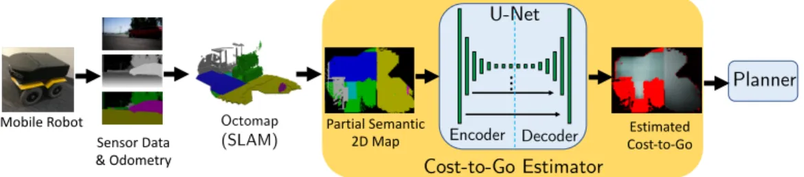
Figure 3-2: System architecture. To plan a path to an unknown goal position be-yond the sensing horizon, a robot’s sensor data is used to build a semantically-colored gridmap. The gridmap is fed into a U-Net to estimate the cost-to-go to reach the unknown goal position. The cost-to-go estimator network is trained offline with anno-tated satellite images. During online execution, the map produced by a mobile robot’s forward-facing camera is fed into the trained network, and cost-to-go estimates inform a planner of promising regions to explore.
dynamic obstacles.
The contributions of this work are (i) a novel formulation of utilizing context for planning as an image-to-image translation problem, which converts the abstract idea of scene context into a planning metric, (ii) an algorithm to efficiently train a cost-to-go estimator on typical, partial semantic maps, which enables a robot to learn from a static dataset instead of a time-consuming simulator, (iii) demonstration of a robot reaching its goal 189% faster than a context-unaware algorithm in simulated environments, with layouts from a dataset of real last-mile delivery domains, and (iv) an implementation of the algorithm on a vehicle with a forward-facing RGB-D + segmentation camera in a high-fidelity simulation. Software for this work is published at https://github.com/mit-acl/dc2g.
3.2
Background
This section formally defines the problem statement solved in this chapter and de-scribes several bodies of work that solve related problems.
3.2.1
Problem Statement
Let an environment be described by a 2D grid of size (ℎ, 𝑤), where each grid cell is occupied by one of 𝑛𝑐 semantic classes (types of objects). The 2D grid is called the
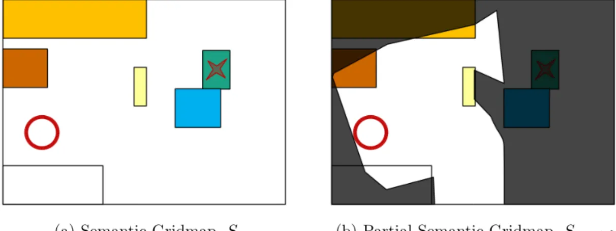
(a) Semantic Gridmap, 𝑆 (b) Partial Semantic Gridmap,𝑆𝑝𝑎𝑟𝑡𝑖𝑎𝑙
Figure 3-3: Problem Statement Visualization. In (a), a red circle indicates an agent inside a semantic gridmap with objects of various semantic class (colored rectangles). The red star denotes the goal region, but the agent is only provided with the goal object class (green object). Furthermore, the agent is not provided with the full environment map a priori – the dark area in (b) depicts regions of the semantic map that have not been observed by the agent yet. As the agent explores the environment, it can use onboard sensors to uncover more of the map to help find the green object.
semantic gridmap, 𝑆 ∈ {1, . . . , 𝑛𝑐}ℎ×𝑤. Let the goal object be one of the semantic
classes, 𝑔𝑐 ∈ {1, . . . , 𝑛𝑐}; the cells in the map of class 𝑔𝑐 is called the goal region,
𝒢 = {(𝑝𝑥, 𝑝𝑦)∈ {1, . . . , 𝑤} × {1, . . . , ℎ}|𝑆𝑝𝑥,𝑝𝑦 = 𝑔𝑐}.
To model the fact that human-built environments are different yet have certain structures in common, let there be a semantic map-generating distribution, S. We populate a training set, 𝒮𝑡𝑟𝑎𝑖𝑛, of maps by taking 𝑁 i.i.d. samples from S, such that
𝒮𝑡𝑟𝑎𝑖𝑛 ={𝑆1, . . . , 𝑆𝑁} ∼ S.
An agent is randomly placed at position p0 = (𝑝𝑥,0, 𝑝𝑦,0) in a previously unseen
test map, 𝑆. The agent does not have access to the full environment map 𝑆; at each timestep 𝑡, the agent can create and use a partial semantic map, 𝑆𝑝𝑎𝑟𝑡𝑖𝑎𝑙,𝑡, using
limited field-of-view/range sensor observations from timesteps 0 ≤ 0 ≤ 𝑡. The agent knows the goal’s semantic class, 𝑔𝑐, but not the goal region, 𝒢. Thus, the observable
state s𝑜
objective of moving the agent to the goal region as quickly as possible, argmin 𝜋 E [𝑡𝑔|s𝑡 , 𝜋, 𝑆] (3.1) 𝑠.𝑡. p𝑡+Δ𝑡 = 𝜋(s𝑜𝑡) (3.2) p𝑡𝑔 ∈ 𝒢 (3.3) 𝑆, 𝑆1, . . . , 𝑆𝑁 ⏟ ⏞ 𝒮𝑡𝑟𝑎𝑖𝑛 ∼ S. (3.4)
This definition formalizes the “ObjectGoal” task defined in [47]. In our work, the agent is not allowed any prior exploration/map of the test environments, but can use the training set to extract properties of the map-generating distribution. The technical problem statement can be visualized in Fig. 3-3.
3.2.2
Related Work
Planning & Exploration
Classical planning algorithms rely on knowledge of the goal coordinates (A*, RRT) and/or a prior map (PRMs, potential fields), which are both unavailable in this problem. Receding-horizon algorithms are inefficient without an accurate heuristic at the horizon, typically computed with goal knowledge. Rather than planning to a destination, the related field of exploration provides a conservative search strategy. The seminal frontier exploration work of Yamauchi provides an algorithm that always plans toward a point that expands the map [26]. Pure exploration algorithms often estimate information gain of planning options using geometric context, such as the work by Stachniss et al. [27]. However, exploration and search objectives differ, meaning the exploration robot will spend time gaining information in places that are useless for the search task.
Context for Object Search
Leveraging scene context is therefore fundamental to enable object search that out-performs pure exploration. Many papers consider a single form of context. Geometric context (represented in occupancy grids) is used in [48–51], but these works also as-sume knowledge of the goal location for planning. Works that address true object search usually consider semantic object relationships as a form of context instead. Joho et al. showed that decision trees and maximum entropy models can be trained on object-based relationships, like positions and attributes of common items in gro-cery stores [28]. Because object-based methods require substantial domain-specific background knowledge, Samadi et al. and Kollar et al. automate the background data collection process by using Internet searches [29, 30]. Object-based approaches have also noted that the spatial relationships between objects are particularly beneficial for search (e.g., keyboards are often on desks) [31–33], but are not well-suited to represent geometries like floorplans/terrains. Hierarchical planners improve search performance via a human-like ability to make assumptions about object layouts [35, 36].
To summarize, existing uses of context either focus on relationships between ob-jects or the environment’s geometry. These approaches are too specific to represent the combination of various forms of context that are often needed to plan efficiently.
Deep Learning for Object Search
Recent works use deep learning to represent scene context. Several approaches con-sider navigation toward a semantic concept (e.g., go to the kitchen) using only a forward-facing camera. These algorithms are usually trained end-to-end (image-to-action) by supervised learning of expert trajectories [37, 39, 52] or reinforcement learning in simulators [40–44]. Training such a general input-output relationship is challenging; therefore, some works divide the learning architecture into a deep neural network for each sub-task (e.g., mapping, control, planning) [39, 42, 43].
general. The difficulty in learning how to extract, represent, and use context in a generic architecture leads to massive computational resource and time requirements for training. In this work, we reduce the dimensionality (and therefore training time) of the learning problem by first leveraging existing algorithms (semantic SLAM, image segmentation) to extract and represent context from images; thus, the learning process is solely focused on context utilization. A second limitation of systems trained on simulated camera images, such as existing deep learning-based approaches, is a lack of transferability to the real world. Therefore, instead of learning from simulated camera images, this work’s learned systems operate on semantic gridmaps which could look identical in the real world or simulation.
Reinforcement Learning
RL, as described in Chapter 2, is a commonly proposed approach for this type of prob-lem [40–44], in which experiences are collected in a simulated environment. However, in this work, the agent’s actions do not affect the static environment, and the agent’s observations (partial semantic maps) are easy to compute, given a map layout and the robot’s position history. This work’s approach is a form of model-based learning, but learns from a static dataset instead of environment interaction.
U-Nets for Context Extraction
U-Nets are a DNN architecture originally introduced by Ronneberger et al. for medical image segmentation [45]. More recently, Isola et al. showed that U-Nets can be used for image translation [16, 53]. This work’s use of U-Nets is motivated by experiments by Pronobis et al. that show generative networks can imagine unobserved regions of occupancy gridmaps [46]. This suggests that U-Nets can be trained to extract significant geometric context in structured environments. However, unlike [46] where the focus of is on models’ abilities to encode context, this work focuses on context utilization for planning.
Semantic Map, !
Dijkstra
Full Cost-to-Go, !"#$
Observation Masks, ℳ
Training Data, &
Satellite View Masked Semantic Maps, !'
Masked Cost-to-Go Images, !"#$' Goal
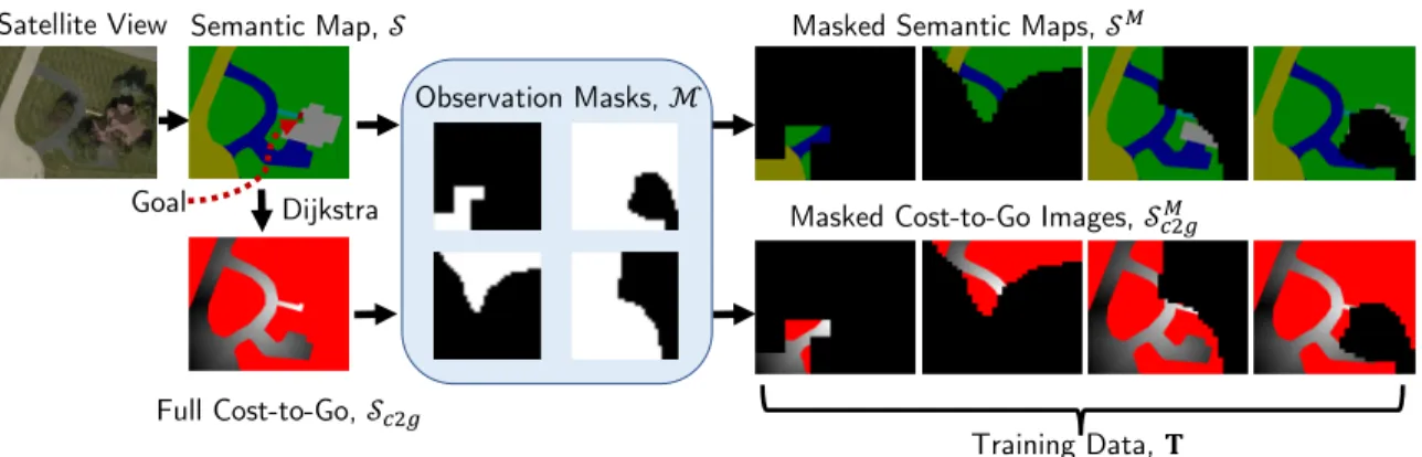
Figure 3-4: Training data creation. A satellite view of a house’s front yard is manually converted to a semantic map (top left), with colors for different objects/terrain. Di-jkstra’s algorithm gives the ground truth distance from the goal to every point along drivable terrain (bottom left) [17]. This cost-to-go is represented in grayscale (lighter near the goal), with red pixels assigned to untraversable regions. To simulate partial map observability, 256 observation masks (center) are applied to the full images to produce the training set.
3.3
Approach
The input to this work’s architecture (Fig. 3-2) is a RGB-D camera stream with semantic mask, which is used to produce a partial, top-down, semantic gridmap. An image-to-image translation model is trained to estimate the planning cost-to-go, given the semantic gridmap. Then, the estimated cost-to-go is used to inform a frontier-based exploration planning framework.
3.3.1
Training Data
A typical criticism of learning-based systems is the challenge and cost of acquiring useful training data. Fortunately, domain-specific data already exists for many ex-ploration environments (e.g., satellite images of houses, floor plans for indoor tasks); however, the format differs from data available on a robot with a forward-facing cam-era. This work uses a mutually compatible representation of gridmaps segmented by terrain class.
A set of satellite images of houses from Bing Maps [54] was manually annotated with terrain labels. The dataset contains 77 houses (31 train, 4 validation, 42 test) from 4 neighborhoods (3 suburban, 1 urban); one neighborhood is purely for training,
Algorithm 1: Automated creation of NN training data
1 Input: semantic maps, 𝒮𝑡𝑟𝑎𝑖𝑛; observability masks, ℳ𝑡𝑟𝑎𝑖𝑛 2 Output: training image pairs, 𝒯𝑡𝑟𝑎𝑖𝑛
3 foreach 𝑆 ∈ 𝒮𝑡𝑟𝑎𝑖𝑛 do
4 𝑆𝑡𝑟 ← Find traversable regions in 𝑆
5 𝑆𝑐2𝑔 ← Compute cost-to-go to goal of all pts in 𝑆𝑡𝑟 6 foreach 𝑀 ∈ ℳ𝑡𝑟𝑎𝑖𝑛 do
7 𝑆𝑐2𝑔𝑀 ← Apply observation mask 𝑀 to 𝑆𝑐2𝑔 8 𝑆𝑀 ← Apply observation mask 𝑀 to 𝑆 9 𝒯𝑡𝑟𝑎𝑖𝑛 ← {(𝑆𝑀, 𝑆𝑐2𝑔𝑀 )} ∪ 𝒯𝑡𝑟𝑎𝑖𝑛
one is split between train/val/test, and the other 2 neighborhoods (including urban) are purely for testing. Each house yields many training pairs, due to the various partial-observability masks applied, so there are 7936 train, 320 validation, and 615 test pairs (explained below). An example semantic map of a suburban front yard is shown in the top left corner of Fig. 3-4.
Algorithm 1 describes the process of automatically generating training data from a set of semantic maps, 𝒮𝑡𝑟𝑎𝑖𝑛. A semantic map, 𝑆 ∈ 𝑆𝑡𝑟𝑎𝑖𝑛, is first separated
into traversable (roads, driveways, etc.) and non-traversable (grass, house) regions, represented as a binary array, 𝑆𝑡𝑟 (Line 4). Then, the shortest path length
be-tween each traversable point in 𝑆𝑡𝑟 and the goal is computed with Dijkstra’s
al-gorithm [17] (Line 5). The result, 𝑆𝑐2𝑔, is stored in grayscale (Fig. 3-4 bottom left:
darker is further from goal). Non-traversable regions are red in 𝑆𝑐2𝑔.
This work allows the robot to start with no (or partial) knowledge of a particular environment’s semantic map; it observes (uncovers) new areas of the map as it ex-plores the environment. To approximate the partial maps that the robot will have at each planning step, full training maps undergo various masks to occlude certain re-gions. For some binary observation mask, 𝑀 ∈ ℳ𝑡𝑟𝑎𝑖𝑛 ⊆ {0, 1}ℎ×𝑤: the full map, 𝑆,
and full cost-to-go, 𝑆𝑐2𝑔, are masked with element-wise multiplication as 𝑆𝑀 = 𝑆∘ 𝑀
and 𝑆𝑀
𝑐2𝑔 = 𝑆𝑐2𝑔∘ 𝑀 (Lines 7 and 8). The (input, target output) pairs used to train
the image-to-image translator are the set of (𝑆𝑀, 𝑆𝑀
3.3.2
Offline Training: Image-to-Image Translation Model
The motivation for using image-to-image translation is that i) a robot’s sensor data history can be compressed into an image (semantic gridmap), and ii) an estimate of cost-to-go at every point in the map (thus, an image) enables efficient use of receding-horizon planning algorithms, given only a high-level goal (“front door”). Although the task of learning to predict just the goal location is easier, a cost-to-go estimate im-plicitly estimates the goal location and then provides substantially more information about how to best reach it.
The image-to-image translator used in this work is based on [16, 53]. The transla-tor is a standard encoder-decoder network with skip connections between correspond-ing encoder and decoder layers (“U-Net”) [45]. The objective is to supply a 256 × 256 RGB image (semantic map, 𝑆) as input to the encoder, and for the final layer of the decoder to output a 256 × 256 RGB image (estimated cost-to-go map, ˆ𝑆𝑐2𝑔). Three
U-Net training approaches are compared: pixel-wise 𝐿1 loss, GAN, and a weighted
sum of those two losses, as in [16].
A partial map could be associated with multiple plausible cost-to-gos, depending on the unobserved parts of the map. Without explicitly modeling the distribution of cost-to-gos conditioned on a partial semantic map, 𝑃 ( 𝑆𝑀
𝑐2𝑔 | 𝑆𝑀), the network
training objective and distribution of training images are designed so the final decoder layer outputs a most likely cost-to-go-map, ¯𝑆𝑀
𝑐2𝑔, where ¯ 𝑆𝑀 𝑐2𝑔 = argmax 𝑆𝑀 𝑐2𝑔∈R256×256×3 𝑃 (𝑆𝑀 𝑐2𝑔 | 𝑆𝑀). (3.5)
3.3.3
Online Mapping: Semantic SLAM
To use the trained network in an online sense-plan-act cycle, the mapping system must produce top-down, semantic maps from the RGB-D camera images and seman-tic labels available on a robot with a forward-facing depth camera and an image segmentation algorithm [55]. Using [56], the semantic mask image is projected into the world frame using the depth image and camera parameters to produce a
point-Algorithm 2: Deep Cost-to-Go (DC2G) Planner
1 Input: current partial semantic map 𝑆, pose (𝑝𝑥, 𝑝𝑦, 𝜃) 2 Output: action u𝑡
3 𝑆𝑡𝑟 ← Find traversable cells in 𝑆
4 𝑆𝑟 ← Find reachable cells in 𝑆𝑡𝑟 from (𝑝𝑥, 𝑝𝑦)w/ BFS 5 if goal ̸∈ 𝑆𝑟 then
6 𝐹 ← Find frontier cells in 𝑆𝑟
7 𝐹𝑒 ← Find cells in 𝑆𝑟 where 𝑓 ∈ 𝐹 in view 8 𝐹𝑟𝑒 ← 𝑆𝑟∩ 𝐹𝑒: reachable, frontier-expanding cells 9 𝑆ˆ𝑐2𝑔 ← Query generator network with input 𝑆 10 𝐶 ← Filter and resize ˆ𝑆𝑐2𝑔
11 (𝑓𝑥, 𝑓𝑦)← argmax𝑓 ∈𝐹𝑒 𝑟 𝐶
12 u𝑡:∞ ← Backtrack from (𝑓𝑥, 𝑓𝑦) to (𝑝𝑥, 𝑝𝑦) w/ BFS 13 else
14 u𝑡:∞ ← Shortest path to goal via BFS
cloud, colored by the semantic class of the point in 3-space. Each pointcloud is added to an octree representation, which can be converted to a octomap (3D occupancy grid) on demand, where each voxel is colored by the semantic class of the point in 3-space. Because this work’s experiments are 2D, we project the octree down to a 2D semantically-colored gridmap, which is the input to the cost-to-go estimator.
3.3.4
Online Planning: Deep Cost-to-Go
This work’s planner is based on the idea of frontier exploration [26], where a frontier is defined as a cell in the map that is observed and traversable, but whose neighbor has not yet been observed. Given a set of frontier cells, the key challenge is in choosing which frontier cell to explore next. Existing algorithms often use geometry (e.g., frontier proximity, expected information gain based on frontier size/layout); we instead use context to select frontier cells that are expected to lead toward the destination.
The planning algorithm, called Deep Cost-to-Go (DC2G), is described in Algo-rithm 2. Given the current partial semantic map, 𝑆, the subset of observed cells that are also traversable (road/driveway) is 𝑆𝑡𝑟 (Line 3). The subset of cells in 𝑆𝑡𝑟 that are
also reachable, meaning a path exists from the current position, through observed, traversable cells, is 𝑆𝑟 (Line 4).
The planner opts to explore if the goal cell is not yet reachable (Line 6). The cur-rent partial semantic map, 𝑆, is scaled and passed into the image-to-image translator, which produces a 256 × 256 RGB image of the estimated cost-to-go, ˆ𝑆𝑐2𝑔 (Line 9).
The raw output from the U-Net is converted to HSV-space and pixels with high value (not grayscale ⇒ estimated not traversable) are filtered out. The remaining grayscale image is resized to match the gridmap’s dimensions with a nearest-neighbor interpo-lation. The value of every grid cell in the map is assigned to be the saturation of that pixel in the translated image (high saturation ⇒ “whiter” in grayscale ⇒ closer to goal).
To enforce exploration, the only cells considered as possible subgoals are ones which will allow sight beyond frontier cells, 𝐹𝑒
𝑟, (reachable, traversable, and
frontier-expanding), based on the known sensing range and FOV. The cell in 𝐹𝑒
𝑟 with highest
estimated value is selected as the subgoal (Line 11). Since the graph of reachable cells was already searched, the shortest path from the selected frontier cell to the current cell is available by backtracking through the search tree (Line 12). This backtracking procedure produces the list of actions, u𝑡:∞ that leads to the selected frontier cell.
The first action, u𝑡 is implemented and the agent takes a step, updates its map with
new sensor data, and the sense-plan-act cycle repeats. If the goal is deemed reachable, exploration halts and the shortest path to the goal is implemented (Line 14). However, if the goal has been observed, but a traversable path to it does not yet exist in the map, exploration continues in the hope of finding a path to the goal.
A key benefit of the DC2G planning algorithm is that it can be used alongside a local collision avoidance algorithm, which is critical for domains with dynamic ob-stacles (e.g., pedestrians on sidewalks). This flexibility contrasts end-to-end learning approaches where collision avoidance either must be part of the objective during learning (further increasing training complexity) or must be somehow combined with the policy in a way that differs from the trained policy.
algorithm to confidently “give up” if it fully explored the environment without finding the goal. This idea would be difficult to implement as part of a non-mapping explo-ration algorithm, and could address ill-posed exploexplo-ration problems that exist in real environments (e.g., if no path exists to destination).
3.4
Results
3.4.1
Model Evaluation: Image-to-Image Translation
Training the cost-to-go estimator took about 1 hour on a GTX 1060, for 3 epochs (20,000 steps) with batch size of 1. Generated outputs resemble the analytical cost-to-gos within a few minutes of training, but images look sharper/more accurate as training time continues. This notion is quantified in Fig. 3-6, where generated images are compared pixel-to-pixel to the true images in the validation set throughout the training process.
Loss Functions
Networks trained with three different loss functions are compared on three metrics in Fig. 3-6. The network trained with 𝐿1 loss (green) has the best precision/worst
recall on identification of regions of low cost-to-go (described below). The GAN achieves almost the same 𝐿1 loss, albeit slightly slower, than the networks trained
explicitly to optimize for 𝐿1 loss. Overall, the three networks perform similarly,
suggesting the choice of loss function has minimal impact on this work’s dataset of low frequency images.
Qualitative Assessment
Fig. 3-5 shows the generator’s output on 5 full and 5 partial semantic maps from worlds and observation masks not seen during training. The similarity to the ground truth values qualitatively suggests that the generative network successfully learned the ideas of traversability and contextual clues for goal proximity. Some undesirable
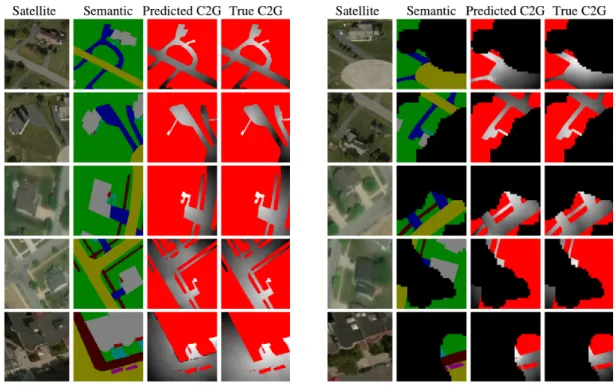
(a) Full Semantic Maps (b) Partial Semantic Maps
Figure 3-5: Qualitative Assessment. Network’s predicted cost-to-go on 10 previously unseen semantic maps strongly resembles ground truth. Predictions correctly assign red to untraversable regions, black to unobserved regions, and grayscale with intensity corresponding to distance from goal. Terrain layouts in the top four rows (suburban houses) are more similar to the training set than the last row (urban apartments). Accordingly, network performance is best in the top four rows, but assigns too dark a value in sidewalk/road (brown/yellow) regions of bottom left map, though the traversability is still correct. The predictions in Fig. 3-5b enable planning without knowledge of the goal’s location.
features exist, like missed assignment of light regions in the bottom row of Fig. 3-5, which is not surprising because in the training houses (suburban), roads and sidewalks are usually far from the front door, but this urban house has quite different topology.
Quantitative Assessment
In general, quantifying the performance of image-to-image translators is difficult [57]. Common approaches use humans or pass the output into a segmentation algorithm that was trained on real images [57]; but, the first approach is not scalable and the second does not apply here.
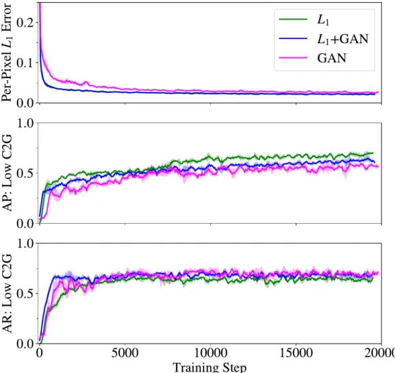
Figure 3-6: Comparing network loss functions. The performance on the validation set throughout training is measured with the standard 𝐿1 loss, and a planning-specific
metric of identifying regions of low cost-to-go. The different training loss functions yield similar performance, with slightly better precision/worse recall with 𝐿1 loss
(green), and slightly worse 𝐿1 error with pure GAN loss (magenta). 3 training
episodes per loss function are individually smoothed by a moving average filter, mean curves shown with ±1𝜎 shading. These plots show that the choice of loss function has minimal impact on this work’s dataset of low frequency images.
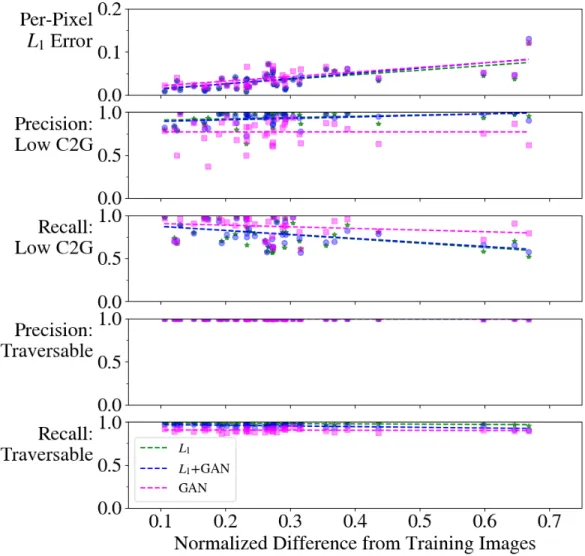
Figure 3-7: Cost-to-Go predictions across test set. Each marker shows the network performance on a full test house image, placed horizontally by the house’s similarity to the training houses. Dashed lines show linear best-fit per network. All three networks have similar per-pixel 𝐿1 loss (top row). But, for identifying regions with
low cost-to-go (2nd, 3rd rows), GAN (magenta) has worse precision/better recall than
networks trained with 𝐿1loss (blue, green). All networks achieve high performance on
estimating traversability (4th, 5th rows). This result could inform application-specific
training dataset creation, by ensuring desired test images occur near the left side of the plot.
Unique to this paper’s domain1, for fully-observed maps, ground truth and
gener-ated images can be directly compared, since there is a single solution to each pixel’s target intensity. Fig. 3-7 quantifies the trained network’s performance in 3 ways, on all 42 test images, plotted against the test image’s similarity to the training images (explained below). First, the average per-pixel 𝐿1 error between the predicted and
true cost-to-go images is below 0.15 for all images. To evaluate on a metric more related to planning, the predictions and targets are split into two categories: pixels that are deemed traversable (HSV-space: 𝑆 < 0.3) or not. This binary classification is just a means of quantifying how well the network learned a relevant sub-skill of cost-to-go prediction; the network was not trained on this objective. Still, the results show precision above 0.95 and recall above 0.8 for all test images. A third metric assigns pixels to the class “low cost-to-go” if sufficiently bright (HSV-space: 𝑉 > 0.9 ∧ 𝑆 < 0.3). Precision and recall on this binary classification task indicate how well the network finds regions that are close to the destination. The networks perform well on precision (above 0.75 on average), but not as well on recall, meaning the networks missed some areas of low cost-to-go, but did not spuriously assign many low cost-to-go pixels. This is particularly evident in the bottom row of Fig. 3-5a, where the path leading to the door is correctly assigned light pixels, but the sidewalk and road are incorrectly assigned darker values.
To measure generalizability in cost-to-go estimates, the test images are each as-signed a similarity score ∈ [0, 1] to the closest training image. The score is based on Bag of Words with custom features2, computed by breaking the training maps
into grids, computing a color histogram per grid cell, then clustering to produce a vocabulary of the top 20 features. Each image is then represented as a normalized histogram of words, and the minimum 𝐿1distance to a training image is assigned that
test image’s score. This metric captures whether a test image has many colors/small regions in common with a training image.
1As opposed to popular image translation tasks, like sketch-to-image, or day-to-night, where
there is a distribution of acceptable outputs.
2The commonly-used SIFT, SURF, and ORB algorithms did not provide many features in this
The network performance on 𝐿1 error, and recall of low cost-to-go regions,
de-clines as images differ from the training set, as expected. However, traversabilty and precision of low cost-to-go regions were not sensitive to this parameter.
Without access to the true distribution of cost-to-go maps conditioned on a par-tial semantic map, this work evaluates the network’s performance on parpar-tial maps indirectly, by measuring the planner’s performance, which would suffer if given poor cost-to-go estimates.
3.4.2
Low-Fidelity Planner Evaluation: Gridworld Simulation
The low-fidelity simulator uses a 50×50-cell gridworld [58] to approximate a real robotic vehicle operating in a delivery context. Each grid cell is assigned a static class (house, driveway, etc.); this terrain information is useful both as context to find the destination, but also to enforce the real-world constraint that robots should not drive across houses’ front lawns. The agent can read the type of any grid cell within its sensor FOV (to approximate a common RGB-D sensor: 90∘ horizontal, 8-cell radial
range). To approximate a SLAM system, the agent remembers all cells it has seen since the beginning of the episode. At each step, the agent sends an observation to the planner containing an image of the agent’s semantic map knowledge, and the agent’s position and heading. The planner selects one of three actions: go forward, or turn ±90∘.
Each gridworld is created by loading a semantic map of a real house from Bing Maps, and houses are categorized by the 4 test neighborhoods. A random house and starting point on the road are selected 100 times for each of the 4 neighborhoods. The three planning algorithms compared are DC2G, Frontier [26] which always plans to the nearest frontier cell (pure exploration), and an oracle (with full knowledge of the map ahead of time).
DC2G and Frontier performance is quantified in Fig. 3-8 by inverse path length. For each test episode 𝑖, the oracle reaches the goal in 𝑙*
𝑖 steps, and the agent following
a different planner reaches the goal in 𝑙𝑖 ≤ 𝑙*𝑖 steps. The inverse path length is thus 𝑙*𝑖 𝑙𝑖,
Training
Houses
Neighborhood
Same
Neighborhood
Different
Urban
Area
Environment Type
0.0
0.2
0.4
0.6
0.8
1.0
Pa
th
Ef
fic
ien
cy
( ora cle act ua l )DC2G
Frontier
Figure 3-8: Planner performance across neighborhoods. DC2G reaches the goal faster than Frontier [26] by prioritizing frontier points with a learned cost-to-go prediction. Performance measured by “path efficiency”, or Inverse Path Length (IPL) per episode, 𝐼𝑃 𝐿 = optimal path length
planner path length. The simulation environments come from real house layouts
from Bing Maps, grouped by the four neighborhoods in the dataset, showing DC2G plans generalize beyond houses seen in training.
per test neighborhood. Because the DC2G and Frontier planners are always expand-ing the map (plannexpand-ing to a frontier point), we see 100% success rate in these scenarios, which makes average inverse path length equivalent to Success Weighted by Inverse Path Length (SPL), a performance measure for embodied navigation recommended by [47].
Fig. 3-8 is grouped by neighborhood to demonstrate that DC2G improved the plans across many house types, beyond the ones it was trained on. In the left category, the agent has seen these houses in training, but with different observation masks applied to the full map. In the right three categories, both the houses and masks are new to the network. Although grouping by neighborhood is not quantitative, the test-to-train image distance metric (above) was not correlated with planner performance, suggesting other factors affect plan lengths, such as topological differences in layout that were not quantified in this work.
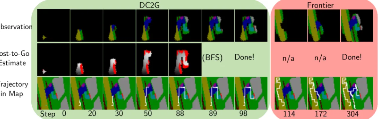
Step 0 20 30 50 88 89 98 (BFS) Done! 114 172 304 DC2G Frontier Done! Observation Cost-to-Go Estimate Trajectory in Map n/a n/a
Figure 3-9: Sample gridworld scenario. The top row is the agent’s observed semantic map (network input); the middle is its current estimate of the cost-to-go (network output); the bottom is the trajectory so far. The DC2G agent reaches the goal much faster (98 vs. 304 steps) by using learned context. At DC2G (green panel) step 20, the driveway appears in the semantic map, and the estimated cost-to-go correctly directs the search in that direction, then later up the walkway (light blue) to the door (red). Frontier (pink panel) is unaware of typical house layouts, and unnecessarily explores the road and sidewalk regions thoroughly before eventually reaching the goal.
Across the test set of 42 houses, DC2G reaches the goal within 63% of optimal, and 189% faster than Frontier on average3.
3.4.3
Planner Scenario
A particular trial is shown in Fig. 3-9 to give insight into the performance improvement from DC2G. Both algorithms start in the same position in a world that was not seen during training. The top row shows the partial semantic map at that timestep (observation), the middle row is the generator’s cost-to-go estimate, and the bottom shows the agent’s trajectory in the whole, unobservable map. Both algorithms begin with little context since most of the map is unobserved. At step 20, DC2G (green box, left) has found the intersection between road (yellow) and driveway (blue): this context causes it to turn up the driveway. By step 88, DC2G has observed the goal cell, so it simply plans the shortest path to it with BFS, finishing in 98 steps. Conversely, Frontier (pink box, right) takes much longer (304 steps) to reach the
3Note that as the world size increases, these path length statistics would appear to make the
Frontier planner seem even worse relative to optimal, since the optimal path would likely grow in length more slowly than the number of cells that must be explored.
goal, because it does not consider terrain context, and wastes many steps exploring road/sidewalk areas that are unlikely to contain a house’s front door.
3.4.4
Unreal Simulation & Mapping
The gridworld is sufficiently complex to demonstrate the fundamental limitations of a baseline algorithm, and also allows quantifiable analysis over many test houses. However, to navigate in a real delivery environment, a robot with a forward-facing camera needs additional capabilities not apparent in a gridworld. Therefore, this work demonstrates the algorithm in a high-fidelity simulation of a neighborhood, using AirSim [59] on Unreal Engine. The simulator returns camera images in RGB, depth, and semantic mask formats, and the mapping software described in Section 3.3 generates the top-down semantic map.
A rendering of one house in the neighborhood is shown in Fig. 3-10a. This view highlights the difficulty of the problem, since the goal (front door) is occluded by the trees, and the map in Fig. 3-10b is rather sparse. The semantic maps from the mapping software are much noisier than the perfect maps the network was trained with. Still, the predicted cost-to-go in Fig. 3-10c is lightest in the driveway area, causing the planned path in Fig. 3-10d (red) from the agent’s starting position (cyan) to move up the driveway, instead of exploring more of the road. The video shows trajectories of two delivery simulations: https://youtu.be/yVlnbqEFct0.
3.4.5
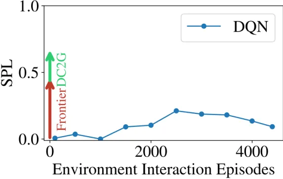
Comparison to RL
We now discuss how an RL formulation compares to our exploration-based planning with a learned context approach. We trained a DQN [60] agent in one of the houses in the dataset (worldn000m001h001) for 4400 episodes. At each step, the RL agent has access to the partial semantic gridmap (2D image) and scalars corresponding to the agent’s position in the gridmap, and its heading angle. We did not succeed in training the agent with just these components as network inputs, but instead pre-processed the observation to assign a white color the agent’s current cell in the gridmap. Thus,
(a) Unreal Engine Rendering of a Last-Mile Delivery
(b) Semantic Map (c) Predicted Cost-to-Go (d) Planned Path
Figure 3-10: Unreal Simulation. Using a network trained only on aerial images, the planner guides the robot toward the front door of a house not seen before, with a forward-facing camera. The planned path (d) starts from the robot’s current posi-tion (cyan) along grid cells (red) to the frontier-expanding point (green) with lowest estimated cost-to-go (c), up the driveway.
0
2000
4000
Environment Interaction Episodes
0.0
0.5
1.0
SPL
Frontier
DC2G
DQN
Figure 3-11: DC2G vs. RL. In blue, an RL agent is trained for 4400 episodes to increase its SPL (efficiency in reaching the goal). With zero training, the Frontier [26] algorithm provides better SPL (red). Instead of training in the environment, DC2G trains on an offline dataset to further improve the performance of a Frontier-based planner. This suggests that planning-based methods could be more effective than RL in these types of navigation problems.
![Figure 3-8: Planner performance across neighborhoods. DC2G reaches the goal faster than Frontier [26] by prioritizing frontier points with a learned cost-to-go prediction.](https://thumb-eu.123doks.com/thumbv2/123doknet/13925343.450136/47.918.163.761.129.479/figure-planner-performance-neighborhoods-frontier-prioritizing-frontier-prediction.webp)