Aircraft Collision Avoidance
Using Monte Carlo Real-Time Belief Space Search
by
Travis Benjamin Wolf
B.S., Aerospace Engineering (2007)
United States Naval Academy
Submitted to the Department of Aeronautics and Astronautics
in partial fulfillment of the requirements for the degree of
Master of Science in Aeronautics and Astronautics
at the
MASSACHUSETTS INSTITUTE OF TECHNOLOGY
May 2009
c
Massachusetts Institute of Technology 2009. All rights reserved.
Author . . . .
Department of Aeronautics and Astronautics
May 22, 2009
Certified by . . . .
James K. Kuchar
Associate Group Leader, Lincoln Laboratory
Thesis Supervisor
Certified by . . . .
John E. Keesee
Senior Lecturer
Thesis Supervisor
Accepted by . . . .
David L. Darmofal
Professor of Aeronautics and Astronautics
Associate Department Head
Chair, Committee on Graduate Students
Aircraft Collision Avoidance
Using Monte Carlo Real-Time Belief Space Search
by
Travis Benjamin Wolf
Submitted to the Department of Aeronautics and Astronautics on May 22, 2009, in partial fulfillment of the
requirements for the degree of
Master of Science in Aeronautics and Astronautics
Abstract
This thesis presents the Monte Carlo Real-Time Belief Space Search (MC-RTBSS) algorithm, a novel, online planning algorithm for partially observable Markov decision processes (POMDPs). MC-RTBSS combines a sample-based belief state representa-tion with a branch and bound pruning method to search through the belief space for the optimal policy. The algorithm is applied to the problem of aircraft collision avoidance and its performance is compared to the Traffic Alert and Collision Avoid-ance System (TCAS) in simulated encounter scenarios. The simulations are generated using an encounter model formulated as a dynamic Bayesian network that is based on radar feeds covering U.S. airspace. MC-RTBSS leverages statistical information from the airspace model to predict future intruder behavior and inform its maneuvers. Use of the POMDP formulation permits the inclusion of different sensor suites and aircraft dynamic models.
The behavior of MC-RTBSS is demonstrated using encounters generated from an airspace model and comparing the results to TCAS simulation results. In the sim-ulations, both MC-RTBSS and TCAS measure intruder range, bearing, and relative altitude with the same noise parameters. Increasing the penalty of a Near Mid-Air Collision (NMAC) in the MC-RTBSS reward function reduces the number of NMACs, although the algorithm is limited by the number of particles used for belief state pro-jections. Increasing the number of particles and observations used during belief state projection increases performance. Increasing these parameter values also increases computation time, which needs to be mitigated using a more efficient implementa-tion of MC-RTBSS to permit real-time use.
Thesis Supervisor: James K. Kuchar
Title: Associate Group Leader, Lincoln Laboratory Thesis Supervisor: John E. Keesee
Acknowledgments
This work was supported under Air Force contract number FA8721-05-C-0002. In-terpretations, opinions, and conclusions are those of the authors and do not reflect the official position of the United States Government. This thesis leverages airspace encounter models that were jointly sponsored by the U.S. Federal Aviation Adminis-tration, the U.S. Air Force, and the U.S. Department of Homeland Security.
I would like to thank MIT Lincoln Laboratory Division 4, led by Dr. Bob Shin, for supporting my research assistantship, and in particular Group 42, led by Jim Flavin, for providing a productive and supportive work environment.
Words cannot express my gratitude for Dr. Jim Kuchar, Assistant Group Leader of Group 43 and my Lincoln Laboratory thesis supervisor, for providing me the op-portunity to pursue graduate studies and for his time, effort, and support in this project. Despite his schedule, Dr. Kuchar provided timely feedback and guidance that ensured my success in this endeavor.
I extend my sincerest thanks to Mykel Kochenderfer of Group 42 for his time and tireless efforts on this project. He provided extensive support and guidance during all phases of this work and never hesitated to rush to assist whenever requested.
I would like to thank Dan Griffith, Leo Espindle, Matt Edwards, Wes Olsen, and James Chryssanthacopoulos of Group 42 for their technical and moral support during my time at Lincoln. My appreciation also goes to Vito Cavallo, Mike Carpenter, and Loren Wood of Group 42 for their invaluable support and expertise.
I would also like to acknowledge COL John Keesee, USAF (Ret.), my academic advisor, for his help in ensuring my smooth progression through MIT.
I would like to thank my parents, Jess, Nicky, and Jorge for their support and encouragement. Thanks also to my friends and partners at Houghton Management for ensuring that my MIT education was complete, quite literally “mens et manus.” A special thanks goes to Philip “Flip” Johnson, without whose early assistance this would not have been possible. Last, I would like to thank Leland Schulz, Vincent Bove, and my other shipmates for their service in harm’s way.
Contents
1 Introduction 15
1.1 Aircraft Collision Avoidance Systems . . . 16
1.1.1 Traffic Alert and Collision Avoidance System . . . 16
1.1.2 Autonomous Collision Avoidance . . . 17
1.2 Challenges . . . 18
1.3 POMDP Approach . . . 19
1.3.1 POMDP Solution Methods . . . 21
1.3.2 Online Solution Methods . . . 22
1.4 Proposed Solution . . . 23
1.5 Thesis Outline . . . 24
2 Partially-Observable Markov Decision Processes 27 2.1 POMDP Framework . . . 28
2.2 Representing Uncertainty . . . 28
2.3 The Optimal Policy . . . 29
2.4 Offline Algorithms: Discrete POMDP Solvers . . . 31
2.5 Online Algorithms: Real-Value POMDP Solvers . . . 32
2.5.1 Real-Time Belief Space Search . . . 32
2.5.2 Monte Carlo POMDPs . . . 33
3 Monte Carlo Real-Time Belief Space Search 35 3.1 Belief State Valuation . . . 35
3.2.1 Belief State Projection . . . 38
3.2.2 Particle Filtering . . . 39
3.2.3 MC-RTBSS Recursion . . . 39
3.2.4 Pseudocode . . . 40
3.2.5 Complexity . . . 42
3.3 Collision Avoidance Application Domain . . . 43
3.3.1 Encounter Models . . . 43
3.3.2 Simulation Environment . . . 47
3.3.3 MC-RTBSS Parameters . . . 54
4 Simulation Results 57 4.1 Simple Encounter Cases . . . 57
4.2 Single Encounter Simulation Results . . . 60
4.2.1 TCAS . . . 61
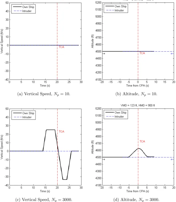
4.2.2 Varying Number of Particles, Np . . . 61
4.2.3 Varying Number of Observations, No . . . 63
4.2.4 Varying NMAC Penalty, λ . . . 65
4.2.5 Varying Maximum Search Depth, D . . . 67
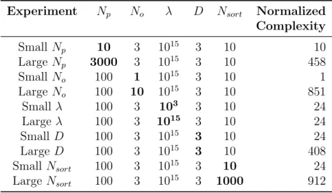
4.2.6 Varying Number of Particles in the Action Sort Function, Nsort 67 4.2.7 Discussion . . . 71
4.3 Large Scale Simulation Results . . . 72
4.3.1 Cost of NMAC, λ . . . 73 4.3.2 Number of Particles, Np . . . 77 4.3.3 Number of Observations, No . . . 81 4.3.4 Discussion . . . 85 5 Conclusion 87 5.1 Summary . . . 87 5.2 Contributions . . . 88 5.3 Further Work . . . 89
List of Figures
2-1 POMDP model. . . 28
2-2 Example of a POMDP search tree. . . 33
3-1 Belief state projection example. . . 38
3-2 Expand example. . . 41
3-3 Dynamic Bayesian network framework for the uncorrelated encounter model. . . 46
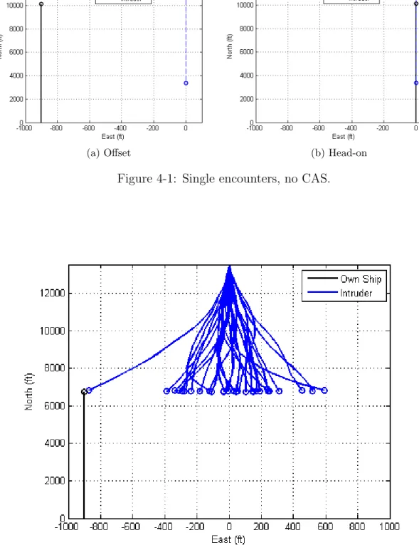
4-1 Single encounters, no CAS. . . 59
4-2 Example intruder trajectories from the encounter model, 20 second duration, offset scenario, no CAS. . . 59
4-3 Single encounter, TCAS. . . 61
4-4 Varying Np, single encounter. . . 62
4-5 Varying No, single encounter. . . 64
4-6 Varying λ, single encounter. . . 66
4-7 Varying D, single encounter. . . 68
4-8 Varying Nsort, single encounter. . . 69
4-9 Examples of generated encounters. . . 74
4-10 Total number of NMACs, varying λ. . . 75
4-11 Mean miss distance, varying λ. . . 76
4-12 Average deviation, varying λ. . . 77
4-13 Miss distance comparison, varying λ. . . 78
4-14 Average deviation comparison, varying λ. . . 78
4-16 Mean miss distance, varying Np. . . 80
4-17 Average deviation, varying Np. . . 81
4-18 Miss distance comparison, varying Np. . . 82
4-19 Average deviation comparison, varying Np. . . 82
4-20 Total number of NMACs, varying No. . . 83
4-21 Mean miss distance, varying No. . . 84
4-22 Average deviation, varying No. . . 85
4-23 Miss distance comparison, varying No. . . 86
List of Tables
2.1 POMDP framework . . . 29
3.1 State variables . . . 48
3.2 Observation variables . . . 48
3.3 Action climb rates . . . 49
3.4 Observation noise model . . . 51
3.5 Tunable parameters . . . 54
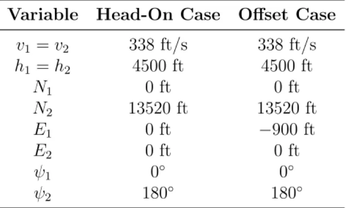
4.1 Single encounter initial conditions . . . 58
4.2 Single encounter MC-RTBSS parameter settings . . . 60
4.3 Nodes expanded . . . 70
4.4 Pruning results . . . 71
4.5 λ sweep values . . . 73
4.6 Np sweep values . . . 77
Nomenclature
General
A Set of actions a Action ai ith action b Belief stateb0 Initial belief state
bt Belief state at time t
ba,o Belief state given action a and observation o
b0a,o Future belief state given action a and observation o
D Maximum search depth
d Current search depth
L Lower bound of V∗
LT Global lower bound within MC-RTBSS instantiation
No Number of observations
Np Number of belief state projection particles
NP F Number of particle filter particles
Nsort Number of sorting function particles
O Observation model
o Observation
oi ith observation
SE State estimator
S Set of states
Sa0 Future set of states given action a
Sa,o,a0 0 Future set of states given action a, observation o, and action a0
s State
si ith state
T Transition function
t Time
tmax Maximum time in simulation
U Utility function
V Value function
Vπ Value function for policy π
V∗ Optimal value function
W Set of belief state particle weights
γ Discount factor
π Action policy
π∗ Optimal policy
Domain Specific
E1 Own ship East displacement
E2 Intruder East displacement
˙
E1 Own ship East velocity component
˙
E2 Intruder East velocity component
h1 Own ship altitude
h2 Intruder altitude
˙
h1 Own ship vertical rate
˙
h2 Intruder vertical rate
N1 Own ship North displacement
N2 Intruder North displacement
˙
N1 Own ship North velocity component
˙
N2 Intruder North velocity component
r Intruder range v1 Own ship airspeed
v2 Intruder airspeed
˙
v1 Own ship acceleration
˙
vhorizontal Horizontal velocity component
wi ith particle weight
β Intruder bearing
θ1 Own ship pitch angle
θ2 Intruder pitch angle
λ Penalty for NMAC
φ1 Own ship bank angle
φ2 Intruder bank angle
ψ1 Own ship heading
ψ2 Intruder heading
˙
ψ1 Own ship turn rate
˙
Chapter 1
Introduction
The Federal Aviation Administration (FAA) Federal Aviation Regulations (FAR) Section 91.113b states:
[R]egardless of whether an operation is conducted under instrument flight rules or visual flight rules, vigilance shall be maintained by each person operating an aircraft so as to see and avoid other aircraft.
This “see and avoid” requirement is of particular concern in the case of unmanned aircraft. While the use of existing collision avoidance systems (CAS) in manned aircraft have been proven to increase the level of safety of flight operations, the use of these systems requires a pilot who can independently verify the correctness of alerts and visually acquire aircraft that the CAS may miss. The lack of an actual pilot in the cockpit to see and avoid presents unique challenges to the unmanned aircraft collision avoidance problem.
Collision avoidance systems rely on noisy, incomplete observations to estimate intruder aircraft state and use models of the system dynamics to predict the future trajectories of intruders. However, current collision avoidance systems rely on rel-atively naive predictions of intruder behavior, typically extrapolating the position of aircraft along a straight line. Most methods also use heuristically chosen safety buffers to ensure that the system will act conservatively in close situations. These assumptions can lead to poor performance including excessive false alarms and flight
path deviation.
More sophisticated models of aircraft behavior exist. For example, an airspace en-counter model is a statistical representation of how aircraft enen-counter each other, de-scribing the geometry and aircraft states during close encounters. Airspace encounter models provide useful information for tracking and future trajectory prediction that has not been incorporated into current collision avoidance systems.
This thesis presents an algorithm called Monte Carlo Real-Time Belief Space Search (MC-RTBSS) that can be applied to the problem of aircraft collision avoid-ance. The algorithm uses a partially-observable Markov decision process (POMDP) formulation with a sample-based belief state representation and may be feasible for online implementation. The general POMDP formulation permits the integration of different aircraft dynamic and sensor models, the utilization of airspace encounter models in a probabilistic transition function, and the tailoring of reward functions to meet competing objectives. This work demonstrates the effect of various parameters on algorithm behavior and performance in simulation.
1.1
Aircraft Collision Avoidance Systems
The Traffic Alert and Collision Avoidance System (TCAS) is the only collision avoid-ance system currently in widespread use. TCAS was mandated for large commercial cargo and passenger aircraft (over 5700 kg maximum takeoff weight or 19 passenger seats) worldwide in 2005 (Kuchar and Drumm, 2007). While TCAS is designed to be an aid to pilots, some preliminary work has commenced on developing automatic col-lision avoidance systems for manned aircraft and colcol-lision avoidance systems designed specifically for autonomous unmanned aircraft.
1.1.1
Traffic Alert and Collision Avoidance System
TCAS is an advisory system used to help pilots detect and avoid nearby aircraft. The system uses aircraft radar beacon surveillance to estimate the range, bearing, relative-altitude, range rate, and relative-altitude rate of nearby aircraft (RTCA, 1997). The
system’s threat-detection algorithms project the relative position of intruders into the future using linear extrapolation, using the estimates of the intruder range-rate and relative-altitude rate. The system also uses a safety buffer to protect against intruder deviations from the nominal projected path. The algorithm declares the intruder as a threat if the intruder is projected to come within certain vertical and horizontal separation limits. If the intruder is deemed to be a threat and the estimated time until the projected closest point of approach (CPA) is between 20 and 48 seconds (depending on the altitude), then TCAS issues a traffic advisory (TA) in the cockpit to aid the pilot in visually acquiring the intruder aircraft. If the intruder is deemed to be a more immediate threat (CPA between 15 and 35 seconds, depending on altitude), then TCAS issues a resolution advisory (RA) to the cockpit, which includes a vertical rate command intended to avoid collision with the intruder aircraft. TCAS commands include specific actions, such as to climb or descend at specific rates, as well as vertical rate limits, which may command not to climb or descend above or below specified rates.
The TCAS threat resolution algorithm uses certain assumptions about the execu-tion of RA commands. The algorithm assumes a 5 second delay between the issuance of the RA and the execution of the command, and that the pilot will apply a 0.25 g vertical acceleration to reach the commanded vertical rate. The algorithm also as-sumes that the intruder aircraft will continue along its projected linear path. However, as the encounter progresses, TCAS may alter the RA to accommodate the changing situation, even reversing the RA (from climb to descend, for example) if necessary. If the intruder aircraft is also equipped with TCAS, then the RA is coordinated with the other aircraft using the Mode S data link. A coordinated RA ensures that the aircraft are not advised to command the same sense (climb or descend) (Kuchar and Drumm, 2007).
1.1.2
Autonomous Collision Avoidance
Some high-performance military aircraft are equipped with the Autonomous Airborne Collision Avoidance System (Auto-ACAS), which causes an Auto-ACAS-equipped
aircraft to automatically execute coordinated avoidance maneuvers just prior to (i.e. the last few seconds before) midair collision (Sundqvist, 2005). Autonomous collision avoidance is an active area of research. One method explored in the literature uses predefined maneuvers, or maneuver automata, to reduce the complexity of having to synthesize avoidance maneuvers online (Frazzoli et al., 2004). The autonomous agent chooses the best automaton using rapidly-expanding random trees (RRTs). Maneuver automata have been used in mixed-integer linear programming (MILP) formulations of the problem, in which the best automaton is that which minimizes some objective function. A MILP formulation has also been used for receding horizon control (Schouwenaars et al., 2004). This method solves for an optimal policy in a given state, assuming some predicted future sequence of states, and chooses the current optimal action. As the agent moves to the next state, the process is repeated, in case some unexpected event occurs in the future. While all of these methods use some sort of dynamic model of the world, the models do not incorporate encounter model data, typically assuming a worst case scenario or simply holding the intruder velocity, vertical rate, and turn rate constant (Kuchar and Yang, 2000). MC-RTBSS incorporates some of the concepts used by many of these methods, such as the use of predefined maneuvers and a finite planning horizon.
1.2
Challenges
While the widespread use of TCAS has increased the safety of air travel (Kuchar and Drumm, 2007), it has some limitations. First, TCAS is ineffective if an intruder is not equipped with a functioning transponder, because it relies upon beacon surveillance. Second, TCAS was designed for use in the cockpit of a manned vehicle, in which there is a pilot who can utilize TCAS alerts to also “see-and-avoid” intruder aircraft; an unmanned aircraft with an automated version of TCAS would rely solely on limited TCAS surveillance for collision avoidance commands. This reliance has several prob-lems, in addition to the possibility of encountering an intruder without a transponder. The information available to TCAS includes coarse altitude discretizations and
par-ticularly noisy bearing observations. In addition, the underlying assumptions of the TCAS algorithms (e.g. linear extrapolated future trajectories) do not necessarily re-flect the reality of the airspace. A better CAS would be able to utilize all information available to verify that the Mode C reported altitude is correct and to provide a bet-ter estimate of the current and future intruder states. Such a CAS would allow for the easy integration of different sensors, such as Electro-Optical/Infra-Red (EO/IR) sensors, Global Positioning System (GPS), or radar, in order to provide the best estimate of the intruder state as possible. In addition, the CAS would utilize the information available in an airspace encounter model to achieve better predictions of the future state of the intruder. Modeling the aircraft collision avoidance problem as a POMDP addresses many of these issues.
1.3
POMDP Approach
A POMDP is a decision-theoretic planning framework that assumes the state is only partially observable and hence, must account for the uncertainty inherent in noisy observations and stochastic state transitions (Kaelbling et al., 1998). A POMDP is primarily composed of four parts: an observation or sensor model, a transition model, a reward function, and a set of possible actions. An agent working under a POMDP framework tries to act in such a way as to maximize the accumulation of future rewards according to the reward function. Beginning with some initial belief state (a probability distribution over the underlying state space), an agent acts and then receives observations. Using models of the underlying dynamics and of its sensors, the agent updates its belief state at each time step and chooses the best action. The solution to a POMDP is the optimal policy, which is a mapping from belief states to actions that maximize the expected future return.
POMDPs have been applied to a wide range of problems, from dynamic pricing of grid computer computation time (Vengerov, 2008) to spoken dialog systems (Williams and Young, 2007). In general, POMDPs are used for planning under uncertainty, which is particularly important in robotics. For example, a POMDP formulation was
used in the flight control system of rotorcraft-based unmanned aerial vehicles (RU-AVs) (Kim and Shim, 2003). A POMDP formulation has also been used for aircraft collision avoidance, resulting in a lower probability of unnecessary alerts (when the CAS issues avoidance maneuvers when no NMAC would occur otherwise) compared to other CAS logic methods (Winder, 2004).
For a POMDP formulation of the aircraft collision avoidance problem, the state space consists of the variables describing the own aircraft position, orientation, rates, and accelerations as well as those of the intruder. The aircraft may receive observa-tions from various sensors related to these variables, such as its own location via a GPS and, in the case of TCAS, the intruder range, bearing, and altitude from the Mode S interrogation responses. The system also has knowledge of the uncertainty associated with these observations; this knowledge is represented in an observation model. The aircraft has an associated set of possible maneuvers, and aircraft dynamic models specify the effect of each maneuver on the aircraft state variables. Use of an airspace encounter model provides the distribution of intruder maneuvers. Both of these pieces constitute the transition model. The reward function is used to score performance, which may involve competing objectives such as avoiding collision and minimizing deviation from the planned path.
In addition to providing an alternative approach to the aircraft collision avoidance problem, the POMDP framework offers advantages compared to previous approaches. First, the use of a reward function facilitates the explicit specification of objectives. The algorithm optimizes performance relative to these objectives. Undesirable events can be penalized in the reward function, while the potentially complex or unknown conditions that lead to the event do not have to be explicitly addressed or even un-derstood; the optimal policy will tend to avoid the events regardless. In addition, the POMDP framework leverages all available information. The use of an explicit transition model allows for the application of airspace encounter models to the under-lying CAS logic. Last, the POMDP framework is very general; a POMDP-based CAS is not tailor-made for a particular sensor system or aircraft platform. Such a CAS could be used on a variety of aircraft with different sensor systems. New sensor suites
can be integrated into or removed from the observation model, which is particularly attractive when an aircraft is equipped with multiple sensors, such as EO/IR sensors, radar, and GPS or undergoes frequent upgrades.
1.3.1
POMDP Solution Methods
POMDP solution methods may be divided into two groups, involving offline and online POMDP solvers. While exact solution methods exist (Cassandra et al., 1994), many methods only approximate the optimal policy.
Offline solvers require large computation time up front to compute the optimal pol-icy for the full belief space. The agent then consults this polpol-icy online to choose actions while progressing through the state space. Offline solvers typically require discrete POMDP formulations. These discrete algorithms take advantage of the structure of the value function (the metric to be maximized) in order to efficiently approximate the value function within some error bound. This type of solution method has sev-eral drawbacks. First of all, the method is insensitive to changes in the environment because the policy is determined ahead of time. Second, the state space of many problems is too rich to adequately represent as a finite set of enumerable states (Ross et al., 2008).
Examples of offline solvers include Point-Based Value Iteration (PBVI), which was applied to Tag, a scalable problem in which the agents must find and tag a moving opponent (Pineau et al., 2003), in addition to other well-known scalable problems from the POMDP literature. PBVI and another offline solver, Heuristic Search Value Iteration (HSVI), were applied to RockSample, which is a scalable problem in which a rover tries to sample rocks for scientific exploration, in addition to other well-known scalable problems found in the POMDP literature, such as Tiger-Grid and Hallway (Smith and Simmons, 2004). HSVI was found to be significantly faster than PBVI in large problems. Successive Approximation of the Reachable Space under Optimal Policies (SARSOP) was applied to robotic tasks, such as underwater navigation and robotic arm grasping (Kurniawati et al., 2008). SARSOP performed significantly faster than the other value iteration algorithms. Offline POMDP solution methods
have recently been applied to the aircraft collision avoidance problem (Kochenderfer, 2009). In particular, this work applied the HSVI and SARSOP discrete POMDP algorithms to the problem. These discrete methods require a reduction in the dimen-sionality of the state space, which inherently results in a loss of information that is useful for the prediction of future states of intruder aircraft.
Online algorithms address the shortcomings of offline methods by only planning for the current belief state. As opposed to planning for all possible situations (as is the case with offline solvers), online algorithms only consider the current situation and a small number of possible plans. Online algorithms are able to account for changes in the environment because they are executed once at each decision point, allowing for updates between these points. In addition, because online algorithms are not solving the complete problem, they do not require a finite state space (as do discrete solvers). Consequently, these algorithms are able to use real-value representations of the state space and are referred to as real-value POMDP solvers. This capability is significant for the aircraft collision avoidance problem because of the large size of the belief space. The use of real values for state variables permits the integration of a wide range of transition functions and sensor models and allows the algorithm to plan for any possible scenario. Attempts to use small enough discretizations to permit the use of such models would cause the problem to be intractable for discrete solution methods.
Paquet’s Real-Time Belief Space Search (RTBSS) is an online algorithm that has been compared to HSVI and PBVI on the Tag and RockSample problems (Paquet et al., 2005b). RTBSS is shown to outperform (achieve greater reward than) HSVI and PBVI in Tag and to perform orders of magnitude faster than these offline al-gorithms. In RockSample, RTBSS performs comparably to HSVI for small problems and outperforms HSVI in large problems.
1.3.2
Online Solution Methods
Two online POMDP solution methods are of particular relevance to this thesis and are mentioned here. First, Real-Time Belief Space Search (RTBSS) (Paquet et al.,
2005b) is an online algorithm that yields an approximately optimal action in a given belief state. Paquet uses a discrete POMDP formulation: a finite set of state variables, each with a finite number of possible values, and a finite set of possible observations and actions. The algorithm essentially generates a search tree, which is formed by propagating the belief state a predetermined depth, D, according to each possible action in each possible reachable belief state. It searches this tree depth-first using a branch and bound method to prune suboptimal subtrees.
Real-time POMDP approaches have been applied to aircraft collision avoidance in the past. Winder (2004) applied the POMDP framework to the aircraft colli-sion avoidance problem, where he assumed Gaussian intruder process noise and used intruder behavioral modes for belief state compression. These modes described the overall behavior of the intruder, such as climbing, level, or descending, to differentiate significant trends in intruder action from noise. Winder showed that a POMDP-based CAS can have an acceptable probability of unnecessary alerts compared to other CAS logic methods.
Thrun (2000) applies a Monte-Carlo approach to POMDP planning that relies upon a sample-based belief state representation. This method permits continuous state and action space representations and non-linear, non-Gaussian transition mod-els.
Monte-Carlo sampling has been used to generate intruder trajectories for aircraft collision avoidance (Yang, 2000). Poisson processes were used to describe the evolu-tion of heading and altitude changes and the resulting probabilistic model of intruder trajectories was used to compute the probability of a future conflict. A CAS could then use this probability to decide whether or not to issue an alert. This process could be executed real-time.
1.4
Proposed Solution
This thesis introduces the Monte Carlo Real-Time Belief Space Search (MC-RTBSS) algorithm. This is a novel, online, continuous-state POMDP approximation
algo-rithm, that may be applied to aircraft collision avoidance. The algorithm combines Paquet’s RTBSS with Thrun’s belief state projection method for sample-based be-lief state representations. The result is a depth-first, branch-and-bound search for the sequence of actions that yields the highest discounted future expected rewards, according to some predefined reward function.
To reduce the computation time, the algorithm attempts to prune sub-trees by using the reward function and a heuristic function to maintain a lower bound for use with a branch and bound method. In addition, the algorithm prunes larger subtrees by using a sorting function to attempt to arrange the actions in order of decreasing expected value. The algorithm uses the resulting ordered set of actions to explore the more promising actions (from a value maximizing perspective) first.
The most significant difference between the new MC-RTBSS presented here and the prior RTBSS is the method of belief state representation. RTBSS assumes a finite number of possible state variable values, observations values, and actions. The algo-rithm then begins to conduct a search of all possible state trajectory-observation pairs. MC-RTBSS, on the other hand, does not assume a finite number of state variable values or observations (though all possible actions are also assumed to be predefined). MC-RTBSS uses a sample-based state representation to represent the belief state as a collection of weighted samples, or particles, where each particle represents a full state consisting of numerous real-valued state values. Each particle is weighted accord-ing to an observation noise model. Instead of iterataccord-ing through each possible future state-observation combination for each state-action pairing, MC-RTBSS generates a specified number of noisy observations, according to an observation model, which is then used to assign weights to the belief state particles. The actual belief state is updated using a particle filter.
1.5
Thesis Outline
This thesis presents MC-RTBSS as a potential real-time algorithm for use in un-manned aircraft collision avoidance systems. This chapter introduced recent methods
of addressing aircraft collision avoidance and discussed methods of CAS analysis. The POMDP framework was suggested as a viable solution to the aircraft avoid-ance problem for unmanned aircraft. This chapter also provided motivation for using MC-RTBSS instead of other POMDP solution methods.
Chapter 2 presents a formal overview of the POMDP framework and a more detailed description of POMDP solution methods. The chapter also discusses Monte-Carlo POMDPs and RTBSS.
Chapter 3 explains the MC-RTBSS algorithm and discusses its implementation in the aircraft collision avoidance application domain. The chapter describes the notation and equations used in the MC-RTBSS transition and observation models as well as the metrics used in the reward function.
Chapter 4 presents results of single encounter scenario simulations with varying parameter settings in addition to the results of parameter sweeps on a collections of encounter simulations.
Chapter 5 presents a summary of this work, conclusions, and suggested further work.
Chapter 2
Partially-Observable Markov
Decision Processes
A partially-observable Markov decision process (POMDP) models an autonomous agent interacting with the world. The agent receives observations from the world and uses these observations to choose an action, which in turn affects the world. The world is only “partially observable,” meaning that the agent does not receive explicit knowledge of the state; it must use noisy and incomplete measurements of the state and knowledge of its own actions to infer the state of the world. In order to accomplish this task, the agent consists of two parts, as shown in Figure 2-1: a state estimator (SE) and a policy (π). The state estimator takes as input the most recent estimate of the state of the world, called the belief state, b; the most recent observation; and the most recent action and updates the belief state. The belief state is a probability distribution over the state space that expresses the agent’s uncertainty as to the true state of the world. The agent then chooses an action according to the policy, which maps belief states to actions. After each time step, the agent receives a reward, determined by the state of the world and the agent’s action. The agent’s ultimate goal is to maximize the sum of expected discounted future rewards (Kaelbling et al., 1998). The state progression of the world is assumed to be Markovian. That is, the probability of transitioning to some next state depends only on the current state (and action); the distribution is independent of all previous states, as shown in Equation
Figure 2-1: POMDP model (Kaelbling et al., 1998).
2.1.
P (st+1| at, st, at−1, st−1, ..., a1, s1) = P (st+1| at, st) (2.1)
2.1
POMDP Framework
A POMDP is defined by the tuple hS, A, T, R, Ω, Oi, where S is the set of states of the world, A is the set of possible agent actions, T is the state-transition function, R is the reward function, Ω is the set of possible observations the agent can receive, and O is the observation function (Kaelbling et al., 1998). The state-transition function, T (s, a, s0), yields a probability distribution over states representing the probability that the agent will end in state s0, given that it starts in state s and takes action a. The reward function, R(s, a), yields the expected immediate reward the agent receives for taking action a from state s. The observation function, O(s0, a, o), yields a probability distribution over observations representing the probability that the agent receives observation o after taking action a and ending up in state s0. The framework is summarized in Table 2.1.
2.2
Representing Uncertainty
The agent’s belief state, b, represents the agent’s uncertainty about the state of the world. The belief state is a distribution over the states that yields the probability that the agent is in state s. At time t, the belief that the system state st is in state
Table 2.1: POMDP framework Notation Meaning S set of states A set of actions T (s, a, s0) state-transition function, S × A → Π(S) R(s, a) reward function, S × A → <
Ω set of possible observations
O(s0, a, o) observation function, S × A → Π(Ω)
s is given by
bt(s) = P (st= s) (2.2)
The belief state is updated each time the agent takes an action and each time the agent receives an observation, yielding the new belief state, b0, calculated as:
b0(s0) = P (s0 | o, a, b) (2.3) = P (o | s 0, a, b)P (s0 | a, b) P (o | a, b) (2.4) = P (o | s 0, a)P s∈SP (s 0 | a, b, s)P (s | a, b) P (o | a, b) (2.5) = O(s 0, a, o)P s∈ST (s, a, s 0)b(s) P (o | a, b) (2.6)
The denominator, P (o | a, b), serves as a normalizing factor, ensuring that b0 sums to unity. Consequently, the belief state accounts for all of the agent’s past history and its initial belief state (Kaelbling et al., 1998).
2.3
The Optimal Policy
As stated earlier, the agent’s ultimate goal is to maximize the expected sum of dis-counted future rewards. The agent accomplishes this by choosing the action that maximizes the value of its current state. The value of a state is defined as the sum of the immediate reward of being in that state and taking a particular action and the discounted expected value of following some policy, π, thereafter, as shown in
Equation 2.7, in which the information inherent in the observation and observation model is utilized: Vπ(s) = R(s, π(s)) + γ X s0∈S T (s, π(s), s0)X o∈Ω O(s0, π(s), o)Vπ(s0) (2.7)
where π is a policy, and π(s) represents the specified action while in state s (i.e. π(s) is a mapping of the current state to an action choice). The optimal policy, π∗ maximizes Vπ(s) at every step, yielding V∗(s):
π∗(s) = arg max a∈A[R(s, a) + γ X s0∈S T (s, π∗(s), s0)X o∈Ω O(s0, π∗(s), o)V∗(s0)] (2.8) V∗(s) = max a∈A[R(s, a) + γ X s0∈S T (s, π∗(s), s0)X o∈Ω O(s0, π∗(s), o)V∗(s0)] (2.9)
However, in most problems the value function is unknown (if it were known, then the problem would be solved). In the case of a POMDP, the agent never knows exactly which state it is in; the agent only has knowledge of its belief state, and hence, the reward function and value function must be evaluated over a belief state, not simply at a single state. The reward associated with a particular belief state is the expected value of the reward function, weighted by the belief state, as shown in Equation 2.10.
R(b, a) =X
s∈S
b(s)R(s, a) (2.10)
The value of a belief state is then computed:
Vπ(b) = R(b, π(b)) + γ
X
o∈Ω
P (o | b, π(b))Vπ(b0o) (2.11)
where b0o is the future belief state weighted according to observation o. A POMDP policy, π(b), specifies an action to take while in a particular belief state b. The solution to a POMDP is the optimal policy, π∗, which chooses the action that maximizes the
value function in each belief state, shown in Equation 2.13. V∗(b) = max a∈A[R(b, a) + γ X o∈Ω P (o | b, a)V∗(b0o)] (2.12) π∗(b) = arg max a∈A[R(b, a) + γ X o∈Ω P (o | b, a)V∗(b0o)] (2.13)
This solution could be reached in finite problems by iterating through every possi-ble combination of actions, future belief states, and observations until some stop point, and then by determining the optimal policy after all of the rewards and probabilities have been determined. However, this process would be unfeasible in even moderately sized POMDPs. Consequently, other solution methods have been devised.
2.4
Offline Algorithms: Discrete POMDP Solvers
Discrete POMDP solution methods, such as Heuristic Search Value Iteration (HSVI) (Smith and Simmons, 2004), Point-based Value Iteration (PBVI) (Pineau et al., 2003), and Successive Approximation of the Reachable Space under Optimal Policies (SAR-SOP) (Kurniawati et al., 2008) require finite state and action spaces. These methods enumerate each unique state (i.e. each possible combination of state variable values) and each unique observation. This discretization allows the transition, observation, and reward functions to be represented as matrices. For example, the transition ma-trix for a given action maps a pair of states to a probability (e.g., the i, jth entry represents the probability of transitioning from the ith state to the jth state). The observation probabilities and reward values can be expressed similarly. These meth-ods approximate the value function as a convex, piecewise-linear function of the belief state. The algorithm iteratively tightens upper and lower bounds on the function until the approximation converges to within some predefined bounds of the optimal value function. Once a value function approximation is obtained, the optimal policy may then be followed by choosing the action that maximizes the function in the current belief state.
2.5
Online Algorithms: Real-Value POMDP Solvers
One significant limitation of a discrete POMDP representation is that the state space increases exponentially with the number of state variables, which gives rise to two significant issues for the aircraft collision avoidance problem: the compact represen-tation of the belief state in a large state space and the real-time approximation of a POMDP solution. Paquet’s Real-Time Belief Space Search (RTBSS) is an online lookahead algorithm designed to compute a POMDP solution. However, the problem of adequate belief state representation still remains. Because of the nature of the Bayesian encounter model and its utilization, the belief state may not necessarily be represented merely by a mean and variance, which would allow for the use of a Kalman filter for belief state update. Thrun’s sample-based belief state representa-tion allows for the adequate representarepresenta-tion of the full richness of the belief state in the aircraft collision avoidance problem, while his particle projection algorithm provides a method to predict future sample-based belief states.
2.5.1
Real-Time Belief Space Search
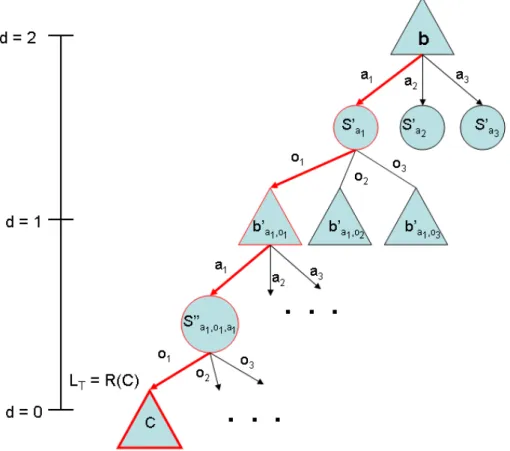
Paquet’s RTBSS is an online algorithm that yields an approximately optimal action in a given belief state. Paquet assumes a discrete POMDP formulation: a finite set of state variables, each with a finite number of possible values, and a finite set of possible observations and actions. In order to reduce the computation time of tradi-tional POMDP approximation methods (e.g. discrete solvers), Paquet uses a factored representation of the belief state. He assumes that the all of the state variables are independent, which allows him to represent the belief state by assigning a probabil-ity to each possible value of each variable, where the the probabilities of the possible values for any variable sum to unity. This factorization provides for the ready identifi-cation of subspaces which cannot exist (i.e. they exist with probability zero). RTBSS uses this formulation to more efficiently search the belief space by not exploring those states which cannot possibly exist from the start of the search. The belief space can be represented as a tree, as in Figure 2-2, by starting at the current belief state, b0, and
Figure 2-2: Example of a POMDP search tree (Paquet et al., 2005a).
considering each action choice, ai, and the possible observations, oj, which may be
perceived afterward. Each action-observation combination will result in a new belief state at the next depth level of the tree. The process is then repeated at each node, resulting in a tree that spans the entire belief space up to some maximum depth level, D. The algorithm searches the tree to determine the optimal policy in the current belief state. At each depth level, RTBSS explores each possible belief state, which depends on (and is calculated according to) the possible perceived observations at that level. The algorithm uses the transition and observation models to determine the belief state variable value probabilities. The goal of the search is to determine which action (taken from the current belief state) yields the highest value. RTBSS uses a branch and bound method to prune subtrees and reduce computation time.
2.5.2
Monte Carlo POMDPs
Thrun’s work with Monte Carlo POMDPs addresses the problem of POMDPs with a continuous state space and continuous action space. A sample-based representation of the belief state is particularly amenable to non-linear, non-Gaussian transition models. Thrun uses such a representation for model-based reinforcement learning in belief space. While MC-RTBSS is not a reinforcement learning algorithm because the observation, transition, and reward models are assumed to be known, Thrun’s
particle projection algorithm is of particular interest. Particle projection is a method of generating a posterior distribution, or the future belief state, for a particular belief state-action pair. The original particle projection algorithm is modified slightly in MC-RTBSS to reduce computation time. Thrun’s original procedure projects a new set of future states for each generated observation. The modified version is shown as Algorithm 1, used to propagate a current belief state forward to the next belief state, given some action. The algorithm projects Np states, sampled from the current
belief state, generates No random observations, and then weights the set of future
states according to each observation, yielding No new belief states. The weights are
normalized according to wn = p(s0n) Np P n=1 p(s0 n) (2.14)
where the probabilities p(s0n) are calculated in line 12 of the particle projection algo-rithm.
Function {b0a,o1, ..., b0a,o
No} = ParticleProject(b, a)
1
Input: b: The belief state to project forward. a: The action. 2 for n = 1 : Np do 3 sample s from b 4 sample s0n according to T (s, a, ·) 5 end 6 for i = 1 : No do 7 sample x from b 8 sample x0 according to T (x, a, ·) 9
sample oi according to O(x0, a, ·) 10
for n = 1 : Np do 11
set particle weight: wn= O(s0n, a, oi) 12
add hs0n, wn0i to b0a,oi
13
end
14
normalize weights in b0a,oi
15
end
16
return {b0a,o1, ..., b0a,oNo}
17
Chapter 3
Monte Carlo Real-Time Belief
Space Search
This chapter discusses the Monte Carlo Real-Time Belief Space Search (MC-RTBSS) algorithm. The algorithm computes the approximately optimal action from the cur-rent belief state. MC-RTBSS is designed for continuous state and observation spaces and a finite action space. The algorithm takes a sample-based belief state represen-tation and chooses the action that maximizes the expected future discounted return. MC-RTBSS uses a branch and bound method, combined with an action sorting pro-cedure, to prune sub-optimal subtrees and permit a real-time implementation.
Section 3.1 presents the belief state representation used by MC-RTBSS. Section 3.2 presents the MC-RTBSS pseudocode and subroutines. Section 3.3 describes the implementation of MC-RTBSS in the aircraft collision avoidance application domain.
3.1
Belief State Valuation
The belief state is a probability distribution over the current state of the system. In order to handle continuous state spaces, the MC-RTBSS algorithm represents the belief state using weighted particles. The belief state, b = hW, Si is a set of state samples, S = {s1, ..., sNp}, and a set of associated weights, W = {w1, ..., wNp}, where
unity. At each time step, the agent must choose an action a from a set of possible actions, A = {a1, ..., a|A|}. The transition function, T (s, a, s0) = P (s0 | s, a), specifies
the probability of transitioning from the current state, s, to some state, s0, when taking action a. At each time step, the agent receives an observation, o, based on the current state. The MC-RTBSS particle filter uses a known observation model, O(s0, a, o) = P (o | s, a), to assign weights to the particles in the belief state. In general, a reward function, R(s, a), specifies the immediate reward the agent receives for being in a particular state s and taking an action a. MC-RTBSS uses its particle representation to approximate the immediate reward associated with a particular belief state: R(b, a) = Np X i=1 wiR(si, a) (3.1)
The value of taking some action ai in a belief state b, V (b, ai), is the expected
dis-counted sum of immediate rewards when following the optimal policy from the belief state. If there are a finite number of possible observations, No, V (b, ai) may be
expressed as: V (b, a) = R(b, a) + γ max a0∈A X o∈Ω P (o | b, a)V (b0o, a0) (3.2)
where Nois the number of generated observations, b0ois the next belief state associated
with the observation o, a0 is the action taken at the next decision point, and γ is a discount factor (generally less than 1). MC-RTBSS is designed to be used with continuous observation spaces that cannot be explicitly enumerated, and so relies upon sampling and a small collection of observations from the distribution P (o | b, a). Equation 3.2 is then approximated by:
V (b, a) = R(b, a) + γ 1 No max a0∈A X o∈Ω V (b0o, a0) (3.3)
Finally, a heuristic utility function, U (b, a), provides an upper bound on the value of being in a particular belief state b and taking a particular action a. As discussed later, MC-RTBSS uses U (b, a) for pruning in its branch and bound method.
3.2
Implementation
MC-RTBSS is implemented in Algorithm 2. The algorithm uses Expand to approxi-mate the optimal action (line 5), which the agent executes before perceiving the next observation and updating the belief state. The initial belief state is represented by b0.
Function OnlinePOMDPAlgorithm()
1
Static: b: The current belief state.
D: The maximum search depth.
action: The best action.
2
b ← b0 3
while simulation is running do
4 Expand(b, D) 5 a ← action 6 Execute a 7
Perceive new observation o
8 b ← ParticleFilter(b, a, o) 9 end 10 Algorithm 2: OnlinePOMDPAlgorithm
MC-RTBSS is implemented as a recursive function that searches for the optimal action at each depth level of the search. The temporal significance (with respect to the environment) of each depth level is determined by the temporal length of an action, because searching one level deeper in the tree corresponds to looking ahead to the next decision point, which occurs when the action is scheduled to be complete. Consequently, the temporal planning horizon of the search is limited to:
tmax = t0+ D × actionLength (3.4)
where t0 is the time at the initial decision point and D is the maximum depth of the
search, which is usually limited by computational constraints.
The belief state at the current decision point is the root node of the aforementioned search tree. MC-RTBSS keeps track of its depth in the search with a counter, d, which is initialized to D and decremented as the depth increases. Thus, at the top of the
Figure 3-1: Belief state projection example.
search tree d = D and at each leaf node d = 0.
3.2.1
Belief State Projection
In order to expand a node, MC-RTBSS executes a modified version of Thrun’s belief state projection procedure. The MC-RTBSS belief state projection pseudocode is shown in Algorithm 1, in Section 2.5.2. When generating a future state for particle projection, the next state, s0 is unknown and must be sampled from T (s, a, ·), where s is sampled from the belief state b. Similarly, when generating an observation in some state s, the observation must be sampled from O(s, a, ·).
This process is illustrated in Figure 3-1. In this example, the search begins at the current belief state b, with MC-RTBSS expanding this node with trial action a1.
The algorithm generates a set of future states by sampling from b and then using the sampled states and a1 to sample a set of future states, Sa01, from T . It also generates
three observations (o1, o2, and o3), which it uses to weight the samples in Sa01, yielding
the three belief states b0a1,o1, b0a1,o2, and b0a1,o3. These belief states are the children of the node b.
3.2.2
Particle Filtering
Belief state update is accomplished using a particle filter. The particle filter algorithm used in this work, ParticleFilter is shown in Algorithm 3. The algorithm takes a belief state, an action, and an observation as its argument and returns a new belief state for the next time step. The particle filter is similar to the ParticleProject, except that it weights the particles according to the perceived observation. NP F is
the number of particles used in the particle filter. Function b0 = ParticleFilter(b, a, o)
1
Input: b: The current belief state. a: The action. o: The observation. 2 for n = 1 : NP F do 3 sample s from b 4 sample s0n according to T (s, a, ·) 5
set particle weight: wn = O(s0n, a, o) 6 add hs0n, w0ni to b0 a,o 7 end 8
normalize weights in b0a,o
9
return b0
10
Algorithm 3: ParticleFilter
3.2.3
MC-RTBSS Recursion
As mentioned earlier, MC-RTBSS is implemented as a recursive function, called Ex-pand, that terminates at some specified depth. The function takes a belief state and a value for its depth, d, as arguments. The function returns both a lower bound on the value of an action choice and an action. After the initial function call, the algorithm is only concerned with the returned value for a given belief state at some depth value (d − 1), which it uses to compute the value of the belief state at the previous depth level (d), according to:
V (b, a) = R(b, a) + γ 1 No No X i=1 Expand(b0a,oi, d − 1) (3.5)
3.2.4
Pseudocode
The full pseudocode of the MC-RTBSS algorithm is introduced in Algorithm 4. Function LT(b) = Expand(b, d)
1
Input: b: The current belief state. d: The current depth.
2
Static: action: The best action.
L: A lower bound on V∗. U : An upper bound on V∗. action ← null 3 if d = 0 then 4 LT(b) ← L(b) 5 else 6
Sort actions {a1, a2, . . . , a|A|} such that U (b, ai) ≥ U (b, aj) if i ≤ j 7
i ← 1
8
LT ← −∞
9
while i ≤ |A| and U (b, ai) > LT(b) do 10 {b0 ai,o1, ..., b 0 ai,oNo} =ParticleProject(b, ai) 11 LT(b, ai) ← R(b, ai) + γN1o PNi=1o Expand(b0ai,oi, d − 1) 12 if LT(b, ai) > LT(b) then 13 action ← ai 14 LT(b) ← LT(b, ai) 15 end 16 i ← i + 1 17 end 18 end 19 return LT(b) 20 Algorithm 4: Expand
In the first D iterations, MC-RTBSS recurs down the first branch of the search tree in a similar manner to a depth-first search. However, when it reaches the first leaf node (when d = 0, node c in Figure 3-2), the algorithm cannot expand any further. As seen in line 5 of Expand, at this point MC-RTBSS calculates a lower bound of the belief state at the leaf node (R(C) in Figure 3-2) and sets it as the lower bound of the search, LT. The algorithm then returns this value to its instantiation at the
previous depth level (d = 1).
The algorithm repeats this process for all of the leaf nodes that are children of the node at depth d = 1 (node b0a1,o1 in Figure 3-2), keeping track of all of these values,
before it reaches line 12, at which point it is able to compute the value associated with taking action a1 in b0a1,o1.
Now that the global lower bound, LT has been updated to something greater than
−∞, the reason for using an upper bound of the actual value of a belief state for the utility function becomes apparent. The result of this evaluation the next time around (U (b, a2), in the case of the example) is compared against the global lower bound
for pruning. Wasting time exploring a suboptimal policy is preferable to pruning the optimal policy, thus it is safer (from an optimality standpoint) to overestimate the value of a leaf node than to underestimate it. The search then iterates through the remaining candidate actions, repeating a similar process unless U (b, ai) ≯ LT, in
which case the node is not expanded for the ith action, effectively pruning the subtree associated with that action. If an action is not pruned and the lower bound obtained from choosing that action is greater than the global bound, then the new action is recorded as the best action, and the global lower bound is updated (line 13).
Until now, the assumption has been that the utility has been computed and that the candidate actions are iterated through in some arbitrary order. However, a sorting procedure is used to compute the utilities of choosing each a while in a given b, and then to order the list of candidate actions in order of decreasing utility. The idea here is that if U (b, ai) > U (b, aj), then ai is more likely to yield a larger value than aj
(i.e. ai is more likely to be part of the optimal policy). If this is indeed the case and
V (bai) > U (b, aj), then the subtree associated with aj and all other ak’s (where k > j)
will be pruned because U yields an upper bound on V (ba) and U (b, aj) ≥ U (b, ak)
(by definition of the sorting function), potentially saving computation time.
After completing the search, the initial instantiation of the search (at d = D) returns both the value approximation of the initial belief state b and the optimal action a.
3.2.5
Complexity
There are (No|A|)d nodes at depth level d in the worst case, where |A| is the number
evaluated by the reward function. In addition, a sorting function is used to order the set of actions by decreasing associated upper bounds (of the value function). This procedure propagates Nsort particles for each of |A| actions at each node. Accounting
for the belief state projection and the sort function at each node, the worst case complexity for MC-RTBSS is bounded by O((Np+ Nsort|A|)(No|A|)D).
3.3
Collision Avoidance Application Domain
This section explains how MC-RTBSS was applied to the problem of collision avoid-ance for unmanned aircraft.
3.3.1
Encounter Models
One of the strengths of the approach to aircraft collision avoidance pursued in this thesis is the leveraging of airspace encounter models, constructed from a large collec-tion of radar data, to predict the future state of intruder aircraft. These encounter models are also used in this thesis to evaluate the performance of the algorithms. This section provides some background on encounter models and their construction.
Encounter Modeling Background
Historically, encounter models have been used by organizations such as the FAA and International Civil Aviation Organization (ICAO) to test CAS effectiveness across a wide range of encounter situations. The encounters generated by the models repre-sent the behavior of aircraft during the final minute or so before a potential collision. The models assume that prior airspace safety layers, such as air traffic control advi-sories, have failed. The encounters are defined by a set of initial conditions for each aircraft and a scripted sequence of maneuvers to occur during simulation. The ini-tial conditions consist of the iniini-tial positions, velocities, and attitudes of the aircraft, and the maneuvers (known as controls or events) specify accelerations and turn rates that are scheduled to occur at specific times during the simulation. The distributions from which these initial conditions and controls are drawn are based on radar data
(Kochenderfer et al., 2008c). A simulation then applies sensor and CAS algorithm models to the aircraft trajectories, allowing the CAS to issue avoidance maneuvers if appropriate, and propagates the aircraft states accordingly. Large numbers of encoun-ters are generated and run in simulation to evaluate performance metrics such as the probability of a Near Mid-Air Collision (NMAC) or the risk ratio, which compares the probability of NMAC of different systems. In the collision avoidance community, an NMAC is an incident in which two aircraft have less than 500 ft horizontal separation and less than 100 ft vertical separation (Kuchar and Drumm, 2007).
Prior Encounter Models
MITRE initially developed an encounter model of the U.S. airspace in the early 1980’s for the development and certification of TCAS in support of the U.S. mandate to equip large transport aircraft with the system (The MITRE Corporation, 1983). This two-dimensional model was used to simulate aircraft vertical motion. The ICAO and Eurocontrol then completed a three-dimensional aircraft model in 2001, which allowed for a single period of acceleration during each encounter. This model was used in support of the worldwide TCAS mandates (Aveneau and Bonnemaison, 2001). Beginning in 2006, new U.S. encounter models were developed for use in the evaluation of TCAS and future CAS for both manned and unmanned aircraft. These models involved collecting and processing data from 130 radars in the U.S. (Kochenderfer et al., 2008a,b,c; Edwards et al., 2009).
Correlated and Uncorrelated Encounters
The availability and presence of air traffic control (ATC) services, such as flight-following services, have an impact on aircraft behavior during encounters. For ex-ample, when both aircraft in an encounter each have a transponder and at least one aircraft is in contact with ATC, then ATC is likely tracking both aircraft and at least one of the aircraft will probably receive notification about nearby traffic. This aircraft may then begin to act accordingly in order to avoid the traffic conflict before any CAS becomes involved. The ATC intervention in the encounter likely
re-sults in some correlation between the two aircraft trajectories. An airspace encounter model that captures such statistically related behavior is called a correlated encounter model. Conversely, a different, uncorrelated encounter model captures the behavior of aircraft in encounters in which there is no prior ATC intervention. This type of encounter includes situations where two aircraft are flying under visual flight rules (VFR) without ATC flight-following or where one of the aircraft is not equipped with a transponder. In these encounters, pilots must visually acquire the other aircraft at close range or use some other CAS in order to avoid collision, generally resulting in uncorrelated trajectories. The uncorrelated encounter model captures this type of behavior by randomly propagating the aircraft trajectories based solely on the statistical characteristics of the individual aircraft (Kochenderfer et al., 2008c).
Encounter Model Construction and Implementation
Encounter models are used to specify the values of certain state variables during sim-ulation. Both the correlated and uncorrelated encounter models describe the true airspeeds, airspeed accelerations, vertical rates, and turn rates of each aircraft in-volved in an encounter. The models also include environmental variables for aircraft altitude layer and airspace class. The correlated model includes the approach an-gle, horizontal miss distance, and vertical distance at the time of closest approach (Kochenderfer et al., 2008a).
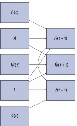
The encounter models use Markov processes to describe how the state variables change over time. A Markov process assumes that the probability of a specific future state only depends on the current state. In short, the process assumes the future is independent of the past. Dynamic Bayesian networks are then used to express the statistical interdependencies between variables (Neapolitan, 2004). As an example, the structure of the dynamic Bayesian network used for the uncorrelated encounter model is shown in Figure 3-3.
The arrows between the variables represent direct statistical dependencies between the variables. The vertical rate, ˙h, turn rate, ˙ψ, and linear acceleration, ˙v, vary with time. The airspace class, A, and altitude layer, L, are characteristic of each
Figure 3-3: Dynamic Bayesian network framework for the uncorrelated encounter model (Kochenderfer et al., 2008b).
encounter and do not vary with time. The first set of variables (on the left of Figure 3-3) represents the variable values at the current time (time t). The second set of variables (on the right of Figure 3-3) represents the variable values at the next time step (time t + 1). Each of the variables in the second set (the variable values at the next time step) have an associated conditional probability table. The values of these tables are determined by statistics derived from collected radar data. The dynamic Bayesian network is then used to generate encounter trajectories by sampling from the network according to the conditional probability tables (in accordance with the previous variable values) and projecting the aircraft states forward accordingly. The particular structure used for the encounter models was not chosen haphazardly. The structure was chosen and optimized according to a quantitative metric, the Bayesian scoring criterion, which is related to the likelihood that the set of radar data would be generated from the network (Kochenderfer et al., 2008b; Neapolitan, 2004).
3.3.2
Simulation Environment
MC-RTBSS was integrated into existing fast-time simulation infrastructure, MIT Lin-coln Laboratory’s Collision Avoidance System Safety Assessment Tool (CASSATT). CASSATT is implemented in the Simulink environment, permitting the easy appli-cation of specific aircraft dynamics models and limits as well as the incorporation of different sensor models and CAS algorithms. Up to millions of encounters are generated using an encounter model and simulated in CASSATT using a parallel computing cluster to test the performance of various collision avoidance algorithms (Kochenderfer et al., 2008c). The dynamic simulation operates at 10 Hz, while MC-RTBSS operates at 1 Hz, beginning at t = 4 s. The first 3 seconds are used to generate an initial belief state, described later, which is fed into the particle filter to be updated using the latest observation. The resulting belief state is then fed into the MC-RTBSS algorithm. The uncorrelated airspace encounter model represents encounters in which aircraft must rely solely on the ability to “see-and-avoid” intruders. These situations present one of the greatest challenges to integrating unmanned aircraft into the U.S. airspace.
States
The MC-RTBSS state is comprised of a vector of 21 state variables: 10 variables for each of the aircraft (the own aircraft and the intruder aircraft) and one variable for the simulation time. This vector is shown below
s = hv1, N1, E1, h1, ψ1, θ1, φ1, ˙v1, ˙h1, ˙ψ1, v2, N2, E2, h2, ψ2, θ2, φ2, ˙v2, ˙h2, ˙ψ2, ti (3.6)
where the subscripts 1 and 2 correspond to the own aircraft and the intruder aircraft, respectively. The definition and units for each variable are shown in Table 3.1.
Table 3.1: State variables
Variable Definition Units
v airspeed ft/s
N North displacement ft
E East displacement ft
h altitude ft
ψ heading rad
θ pitch angle rad
φ bank angle rad
˙v acceleration ft/s2
˙h vertical rate ft/s
˙
ψ turn rate rad/s
Observations
An observation is comprised of the following four elements:
o = hr, β, h1, h2i (3.7)
The definition and units for each are shown in Table 3.2. Table 3.2: Observation variables
Variable Definition Units
r slant range ft
β bearing rad
h1 own altitude ft
h2 intruder altitude ft
Bearing is measured clockwise from the heading of the own aircraft. The range and bearing can be determined from the state variables using the following operations:
r =p(N2− N1)2+ (E2− E1)2+ (h2− h1)2 (3.8)
β = arctan2(E2− E1, N2− N1) − ψ1 (3.9)
Actions
The set of all possible actions, A, contains 6 actions at any given decision point. Each action, in turn, consists of a sequence of 5 commands, each of which is meant to be executed each second, beginning at a decision point and finishing 5 seconds later, should that action be chosen. In the simulations conducted in this project, one of the 6 candidate actions is always the nominal set of commands for that 5 seconds of time in the simulation (i.e. the 5 entries describing the aircraft’s default behavior, sampled from the encounter model). Every other candidate action has the same acceleration and turn rate ( ˙v and ˙ψ, respectively) as the nominal commands, but the vertical rate ( ˙h) is different. The vertical rates for all of the actions are described in Table 3.3.
Table 3.3: Action climb rates
Action Climb Rate (ft/min)
a1 2000 a2 1500 a3 0 a4 −1500 a5 −2000 a6 scripted Transition Function
The transition function, T , takes a state and an action as its arguments and deter-ministically propagates the own ship state variables forward by using simple Euler integrations, shown below, using the chosen action to determine the rates at each time step (∆t = 1 s).
vn+1 = vn+ ˙vn+1∆t (3.10)
hn+1 = hn+ ˙hn+1∆t (3.11)
The transition function calculates the flight path angle θ at each instant using the trigonometric relations of other state variables at that instant.
θ = sin−1 ˙h
v (3.13)
The transition function propagates aircraft location through space by determining the horizontal component of velocity, vhorizontal, and then breaking this vector into
its North and East components ( ˙N and ˙E, respectively). These components are then used in an Euler integration to propagate the aircraft in the respective directions. The transition function does not model vertical acceleration (¨h), bank angle (φ), angular rates (p,q,r) or accelerations ( ˙p, ˙q, ˙r) and consequently, the transition function is unable to model aircraft performance limitations on these variables.
vhorizontal = v cos θ (3.14) ˙ N = vhorizontalcos ψ (3.15) ˙ E = vhorizontalsin ψ (3.16) Nn+1 = Nn+ ˙N ∆t (3.17) En+1 = En+ ˙E∆t (3.18)
The function calls another function, GenerateIntruderAction, which takes the state at a particular time step as its argument and uses the intruder action and altitude at some time t to sample the intruder action at time t + 1 from the encounter model. The function repeats this procedure for the duration of the own ship action. The transition function returns a state trajectory of duration equal to the input action duration.
Observation Model
MC-RTBSS needs to be able to generate observations from the observation model and consult the posterior distributions (of the observation components) to determine weights for the samples that comprise a belief state. In order to achieve these goals,


![[PDF] Cours marché des changes pdf : les risques | Cours Forex](data:image/gif;base64,R0lGODlhAQABAIAAAP///wAAACH5BAEAAAAALAAAAAABAAEAAAICRAEAOw==)