Automated Feedback in Flow for Accelerated Reaction Screening,
Optimization, and Kinetic Parameter Estimation
by
Brandon Jacob Reizman
B.S. Chemical Engineering, University of Illinois at Urbana-Champaign (2009) M.S. Chemical Engineering Practice, Massachusetts Institute of Technology (2011)
Submitted to the Department of Chemical Engineering in Partial Fulfillment of the Requirements for the Degree of
Doctor of Philosophy in Chemical Engineering at the
MASSACHUSETTS INSTITUTE OF TECHNOLOGY
May 2015 [VIe 2O151
0 2015 Massachusetts Institute of Technology. All rights reserved
Signature of Author...
Signature
Certified by ... , W LC) (/) zj - < 0 0L C -0 U c U)jSignature redacted
Department of Chemical EngineeringMay 15, 2015
redacted
Klavs F. Jensen Warren K. Lewis Professor of Chemical Engineering Professor of Materials Science and Engineering Thesis Supervisor
A ccepted by ...
Signature redacted
Richard D. Braatz Edwin R. Gilliland Professor of Chemical Engineering Chairman, Committee for Graduate StudentsAutomated Feedback in Flow for Accelerated Reaction Screening,
Optimization, and Kinetic Parameter Estimation
Brandon Jacob Reizman
ABSTRACT
With the cost to discover and develop a drug now estimated to exceed $2 billion, the pharmaceutical industry is in search of innovative and cost-effective ways to reduce process footprint, minimize lead times, and accelerate scale-up. One path to achieving these goals is in the adoption of continuous processing. Among the many advantages offered by the use of continuous flow systems is the ease of integration of automation and online analytics for real-time monitoring of reactions. The further incorporation of feedback into automated systems invents an even greater possibility: the use of algorithms to intelligently manipulate different continuous variables-for instance temperature, time, and concentration-until an optimal synthesis is achieved. This thesis opens by reviewing the most recent applications of feedback optimization in flow. The same methodology is then applied to the estimation of reaction kinetics in a series-parallel SNAr reaction network.
Unfortunately, the most challenging aspect of reaction development tends not to necessarily be the continuous variables, but rather the enumerate combinations of discrete variables-e.g. catalysts, ligands, and solvents-that, when paired with the continuous variables, give rise to changes in the reaction mechanism or kinetics. To address this problem, this thesis introduces a more general approach to reaction optimization with the construction of an automated segmented flow system, wherein reactants are confined to sub-20 pL slugs flowing through a heated Teflon tube microreactor and analyzed online by LC/MS. The system allows for manipulation of both discrete and continuous variables, making it possible to simultaneously screen reagents while optimizing the reaction. A sequential adaptive response surface methodology for optimizing both discrete and continuous variables is presented. The algorithm employs optimal design of experiments in feedback to greatly accelerate convergence of the mixed integer nonlinear programming (MINLP). Examples of real-time simultaneous screening and optimization are explored, including optimal solvent selection in a selective alkylation reaction and optimal palladacycle-ligand precatalyst selection for Suzuki-Miyaura cross-coupling reactions. We conclude by showing how the automated system can be utilized to gain further understanding of reaction mechanisms and kinetics and by demonstrating that the optimal results can be scaled to larger chemical syntheses.
Thesis Supervisor: Klavs F. Jensen
Department Head, Chemical Engineering
Warren K. Lewis Professor of Chemical Engineering Professor of Materials Science and Engineering
To my dad, who thought I should be an accountant, and to my mom, who thought otherwise.
ACKNOWLEDGEMENTS
Undoubtedly the person to acknowledge first and foremost for this thesis is my advisor, Prof. Klavs Jensen. He has been a great mentor and supporter of my work, and most of the innovations shared below would have not been possible without either his foresight or the culture of community and knowledge he has fostered in his research group. I still remember sitting in his office in fall 2010, with my thesis proposal looming, wondering what would make for a captivating project to embark on for the rest of my thesis. When Prof. Jensen pitched the idea of simultaneous catalyst screening and reaction optimization, I told him first hand that it sounded like an amazing idea, but that I had no idea how to do it. His response: "that's what makes it a good thesis project."
Beyond Prof. Jensen, I have benefited greatly-both academically and personally-from the mentorship of many others in the MIT community. The faculty in particular have always challenged me to look at problems in new ways and encouraged me to go far beyond what I would have first considered to be a lofty goal. I have received insightful guidance on this research in particular from my thesis committee Prof. Steve Buchwald, Prof. Richard Braatz, and Prof. Paul Barton, as well as another member of the MIT-Novartis collaboration, Prof. Tim Jamison, and the continuous manufacturing group at Novartis led by Dr. Berthold Shenkel. Funding from the Novartis-MIT Center for Continuous Manufacturing made this research possible. As a teaching assistant, I was fortunate to benefit from the mentoring of Prof. Michael Strano and Prof. Hadley Sikes, and much of my ability to deduce problems and effectively communicate solutions can be attributed to the support I received from Prof. Claude Lupis and Prof. Bob Hanlon at Practice School. Through work in the classroom, the rest of the chemical engineering faculty and the MIT faculty on the whole has opened my eyes to new ideas and innovative strategies for problem solving.
I have been privileged to work in research with a group of equally talented and thoughtful colleagues. It is hard to imagine this particular thesis being feasible without the innovativeness of Dr. Jon McMullen and Dr. Jason Moore, who were first to demonstrate the incredible value of automated optimization in flow and were my educators in software development, online instrumentation, and assembling high-throughput systems. Recently, I have benefited immensely from discussions about instrumentation and software from new members of the automation team, Isaac Roes, Kosi Aroh, Connor Coley, and Dr. Milad Abolhasani. Many of the physical
components of the system I demonstrate herein were contributions of the thought, time, and effort of Dr. Andrea Adamo, Dr. Baris Onal, Dr. Everett O'Neal, and Dr. Patrick Heider, along with UROP Michaelann Rodriguez. The micromixer and silicon microreactor used in Chapter 2 were contributions from Dr. Nick Zaborenko and Dr. Lei Gu, respectively. In terms of organic synthesis, my growth as a chemist is forever endeared to Dr. Chris Smith, who tolerated my endless nights of "amateur hour" in hopes that someday I would run a column better than the driver of Jose's Taco Truck (no offense intended to Jose's). I have subsequently benefited from the teachings of Dr. Stephen Born, Prof. Steve Newman, Dr. Saurabh Shahane, and Dr. Antony Fernandes. The impact of my thesis would be far less without the guidance of those in the Buchwald and Jamison groups, in particular Dr. Yiming Wang, Dr. Nick Bruno, and Andy McTeague. Along the way, I have received a great amount of feedback on my research not jist from those listed above, but from the rest of the Jensen chemical synthesis subgroup and the Jensen group on the whole.
Above all, a huge thank you must be extended to those around the MIT community who have supported my growth for the past several years. Thanks in particular go to the support staff in chemical engineering who have worked tirelessly to make my experience at MIT smooth and always enjoyable: Alina Haverty, Suzanne Maguire, Joel Dashnaw, Katie Lewis, Fran Miles, Beth Tuths, Steve Wetzel, and Brian Smith. In my time spent at MIT, I have been a member of some excellent organizations, most notably the MIT Energy Initiative, the Course X Graduate Student Council, the ChemE Graduate Student Advisory Board, the Thirsty Ear Executive Committee, and a host of intramural sports teams. I have benefited immensely from the friendships built through those groups and with other graduate students in chemical engineering, most notably Dr. Caleb Class, Dr. Rathi Srinivas, Dr. Jon Harding, Dr. Dave Borrelli, Dr. Nisarg Shah, Dr. Nigel Reuel, Tim Politano, and Su Zhu. I would like to thank my family, both my sister Caitlyn and my mom and dad for the support and encouragement they have given me not just now but in my entire academic career. And I would like to thank the love and support I have received from a very newly awarded doctor, Dr. Irene Brockman, who has worked harder than anyone to help me reach my fullest potential. Irene, we made it!
TABLE OF CONTENTS A bstract ...---. --... 3 Acknowledgements... ---... 7 Table of Contents... - --- ---...--.-.- 9 List of Figures... ---.---.---... 14 List of Tables ... ---... 19
L ist of Schem es...---- --- ---- ---- - -- -... 22
1. Feedback Systems for the Acceleration of Reaction Development... 25
1.1. The Tools for Feedback Optimization in Flow... 28
1.2. Reaction Optimization "from Scratch"... 31
1.3. Kinetics in Flow: A Route to Faster Scale-up ... 36
1.4. Bringing Discrete Variables into the Optimization ... 37
1.5. Thesis Overview and Goals ... 39
2. An Automated Continuous-Flow Platform for the Estimation of Multi-Step Reaction Kinetics ... . --- ---... 41
2.1. Introduction...- ... ..---... 41
2.2. M ethod ... ---... 42
2.2.1. K inetic M odel ... ...---... 43
2.2.2. Approach to Parameter Estimation ... 45
2.2.3. Approach to Optimal Experimental Design... 47
2.3. Experim ental... ... ---... 48
2.3.1. Automated Parameter Estimation System ... 48
2.3.2. Experimental Design... 50
2.3.3. Synthesis and Isolation of Products ... 53
2.3.4. Automated Calibration of Analyzed Compounds... 55
2.4. R esults... ---... 55
2.4.1. Simultaneous Estimation of Kinetic Parameters... 55
2.4.2. Estimation of Kinetic Parameters from Isolated Reactions ... 58
2.5. D iscussion ... ... 65
3. A Segmented Flow System for On-Demand Screening of Discrete and Continuous
V ariab les ... 72
3 .1. Introd uction ... 72
3 .2 . M eth o d ... 7 7 3.2.1. Automated Reagent Handling... 79
3.2.2. Slug Transport and Reaction... 82
3.2 .3 . O n line Injection ... 85
3.2.4. Quenching and Online Analysis ... 86
3.2 .5 . A utom ation ... 87
3 .3 . E xperim ental... 87
3.3.1. Reagent Stirring and Carryover ... ... 87
3.3.2. "Pancake" Reactor Modeling... 89
3.3.3. Comparison of Reaction Yield in Batch and in Slugs ... 91
3.4. Results and Discussion ... 92
3.4.1. Reagent Stirring and Carryover ... 92
3.4.2. COMSOL Simulations of Heat Transfer in the Pancake Reactor... 95
3.4.3. Comparison of Reaction Yield in Batch and in Slugs ... 97
3 .5 . C o nclusions... 99
4. An Adaptive Response Surface Methodology for Optimization of Discrete and Continuous Variable Chemical Systems ... 101
4 .1. Intro d uctio n ... 10 1 4 .2 . M eth o d ... 10 3 4.2.1. Approach to Real-Time Discrete and Continuous Variable Optimization ... 103
4.2.2. Construction of Discrete Variable-Specific Response Surface Models... 105
4.2.3. Optimization of Response Surface Models and Discrete Variable Fathoming ... 106
4.2.4. Real-Time Experimental Considerations ... 109
4 .3 . R esu lts... 10 9 4.3.1. Test Case 1: The Effect of y upon Convergence... 110
4.3.2. Test Case 2: Optimization with Multiple Discrete Variable Optima... 113
4.3.3. Test Case 3: Perturbations to the Reaction Pathway ... 116
4.4. Conclusions...--- --- --- -- --- --...123
5. Simultaneous Solvent Screening and Reaction Optimization for the Alkylation of 1,2-Diaminocyclohexane... 125
5.1. Introduction... ... ..-... 125
5.2. M ethod ... ... ---... 127
5.3. Experim ental... .... ---... 129
5.3.1. Procedure for On-Demand Solvent Screening... 129
5.3.2. Preparation of (N-4-methoxybenzyl)-(1R,2R)-(-)-diaminocyclohexane (lR,2R-(-)-12) ... ... ---... 130
5.3.3. Automated Reagent Calibration... 131
5.4. R esults... ---... 131
5.5. Discussion...- ... ...- -- - -- - -- - ---... 134
5.6. Conclusions...- - - -- - --... 136
6. Optimization and Kinetic Investigations of Suzuki-Miyaura Cross-Coupling Reactions.. 138
6.1. Introduction...-- -- - -- ---... 138
6.2. M ethod ... ---... 141
6.3. Experimental...-...- - -- - - - --... 141
6.3.1. General Solution Preparation Procedure... 141
6.3.2. Automated Reaction Optimization and Screening... 142
6.3.3. Automated Boronic Acid and Ester Degradation Studies... 143
6.4. Results... --- --- -- -- --- -- - -- - --... 143
6.4.1. Optimization of TON in Suzuki-Miyaura Cross-Coupling Systems ... 143
6.4.2. Optimization of Ligand Equivalents... 148
6.5. Discussion... ... ---... 149
6.5.1. Mechanistic Insights ... 149
6.5.2. Unstable Reactants and Products, and the Correlation to Ligand Selection... 150
6 .6 . C onclusions... . ---... 153
7. Conclusions and Future Research Directions ... 154
7.1. Introduction... ... ... 154
7.2. Sum m ary of Thesis Contributions ... 155
7.3. Future Research D irections... 158
8. N om enclature ... 161
9. References... 164
Appendix A. Chapter 2 Supporting Inform ation ... 185
A . 1. Experim ental Data ... 185
Appendix B. Chapter 3 Supporting Inform ation... 188
B. 1. A utom ated Screening System Standard Operating Procedure... 188
B. l.1. HPLC Initialization ... 188
B.1.2. System Initialization... 189
B.1 .3. List of LabView Files... 191
B.1.4. List of M A TLA B Files... 196
B.2. Devices ... ... 02
B.2.1. V ial M anifold ... 202
B.2.2. Pancake Reactor ... 203
Appendix C. Chapter 4 Supporting Inform ation... 204
C.1. Optim ization Scripts... 204
C.1.1. Optim ization Phase I ... 204
C. 1.2. Optim ization Phase 2 ... 210
C.1 .3. O ptim ization Phase 3 ... 218
C. 1.4. Construction of X M atrix ... 232
C.2. Sim ulation Data... 236
Appendix D . Chapter 5 Supporting Inform ation ... 261
D . 1. Experim ental Data ... 261
D .2. N M R Spectra ... 265
Appendix E. Chapter 6 Supporting Inform ation... 266
E. 1. Experim ental Data... 266
E. 1.1. Reaction of 13 and 14... 266
E.1.2. Calibration of 17... 269
E.1.3. Reaction of 16 and 14... 269
E.1.4. Reaction of 16 and 18... 272
E.1.5. Reaction of 9 and 7... 275
E. 1.7. Time-Course Evolution of 18 and Reaction of 16 and 21... 281 E .2. N M R Spectra ... ... ---... 282
LIST OF FIGURES
Figure 1.1 Generalized feedback loop for (deterministic) automated reaction optimization. ... 27 Figure 1.2. Block diagram for automated feedback optimization in flow systems. ... 28 Figure 1.3. Automated feedback loop used by McMullen et al. for the optimization in Scheme
1 .1.22 ---... ... ... 3 2
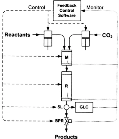
Figure 1.4. Automated system for optimization of the methylation of alcohols introduced by Parrott et al.84
M is a static mixed and R is the reactor packed with catalyst... 34 Figure 1.5. Convergence of the Paul-Knorr reaction from the automated system of Moore and Jensen.58 Diamond-steepest descent algorithm. Circle-conjugate gradient algorithm with fixed step size. Triangle-conjugate gradient algorithm with Armijo step size ... 3 6 Figure 1.6. Feedback loop for the optimization of methane oxidation by Kreutz et al.98 . . . 38
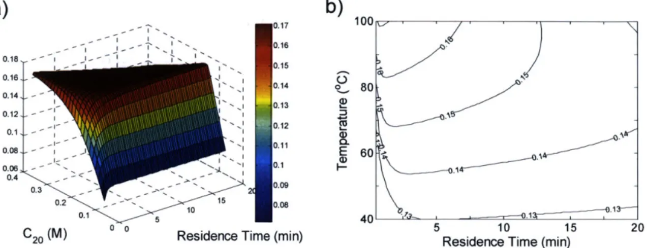
Figure 2.1. Logic flow diagram for automated kinetic parameter estimation in continuous flow. ... 4 3 Figure 2.2. Diagram of the automated continuous-flow parameter estimation system ... 48 Figure 2.3(a-d). Experimental and model-predicted reactant and product concentration profiles after initial factorial design (12 automated experiments). Markers identify experimental data points. Lines indicate model prediction. ... 56 Figure 2.4(a-d). Experimental and model-predicted reactant and product concentration profiles after 24 automated experiments. Markers identify experimental data points. Lines indicate m odel prediction. ... 58 Figure 2.5. (a) Model predicted-yield of 4 with initial concentration Cio = 0.150 M and T = I 000C based upon optimal model parameters for ki and k2 from Table 2.2 and for k3 and k4 from Table 2.1. The ridge of maximum yield is at 17.1%. (b) Model predicted-yield of 4 with initial concentrations Cio = 0.150 M and C2o = 0.375 M based upon optimal model parameters for ki and k2 from Table 2.2 and for k3 and k4 from Table 2.1. The maximum predicted yield is 17.1% at tres = 49 s and T= I 00C. ... 6 1 Figure 2.6(a-f). Experimental and model-predicted reactant and product concentration profiles after completion of all experiments (including simultaneous and isolated
approaches). Markers identify experimental data points. Solid lines indicate model p red ictio n . ... 6 4 Figure 2.7(a-d). 68% and 95% joint confidence regions for estimated parameters after 24 autom ated experim ents ... 67 Figure 2.8(a-d). 68% and 95% joint confidence regions for estimated parameters after all
simultaneous and isolated automated experiments...68 Figure 3.1. Concept diagram for on-demand preparation, reaction, analysis, and feedback in an
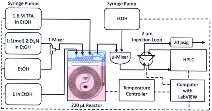
automated reaction flow screening system ... 78 Figure 3.2. Schematic of automated flow system for alkylation reaction optimization... 78 Figure 3.3. Automated system hardware including (a) pumps, automated liquid handler, LC/MS, and automation and (b) reactor and online sampling... 78 Figure 3.4. Septum-sealed inert gas manifold for reagent storage under inert gas atmosphere, (a) SOLIDWORKS rendering and (b) photograph of 3D-printed device... 82 Figure 3.5. Pressure-sealed "pancake" reactor comprising a Teflon tube in an aluminum housing, (a) SOLIDWORKS rendering and (b) photograph of packaged device with polycarbonate cover, FEP tubing, and thermocouple... 84 Figure 3.6. (a) Geometry studied for COMSOL simulations of the pancake reactor and (b) zoomed in view of the Teflon tube cross section. PC = polycarbonate... 90 Figure 3.7. Schematic of reagent sampling and stirring and effect upon calibration reprod ucib ility ... 93 Figure 3.8. (a) Illustration of the effect of pinched tubing upon slug dilution upstream and the effect of (b) pinched and (c) new, un-pinched tubing upon reaction concentration and reproducibility. Black dotted line represents predicted starting material concentration and blue solid line represents observed. The excess conversion in (c) was attributed to not having a quench on the reactor outlet... 94 Figure 3.9. (a) Temperature profile for pancake reactor cross-section for 373.15 K aluminum block and 750 ptm ID FEP tubing after 10 s. (b) Temperature of the center of the channel as a function of vertical position at 5 s (blue), 10 s (green), 20 s (red) and 30 s (aqua). (c) Temperature profile for pancake reactor cross-section for 373.15 K aluminum block and 750 im ID FEP tubing after 10 s after allowing system to equilibrate for 30 s. (d) Temperature of the center of the channel as a function of
vertical position at 5 s (blue), 10 s (green), 20 s (red) and 30 s (aqua) after 30 s of eq u ilibratio n ... 9 6 Figure 3.10. Pancake reactor temperature profile at 373.15 K for (a) surface of the aluminum chuck and (b) cross-section of the chuck with cartridge heaters and polycarbonate co v ers...9 7 Figure 3.11. Comparison of slug flow yields to batch yield for (a) reaction of 2-chlorobenzoxazole and I-boc-2-pyrroleboronic acid with aq. K3PO4 base and (b) reaction of 2-chloropyridine and 1-boc-2-pyrroleboronic acid with DBU base... 98 Figure 4.1. Real-time discrete and continuous variable optimization decision diagram... 104 Figure 4.2. Optimization trajectory for (a) y = 0.90, (b) y = 0.95, and (c) y = 0.98. Catalyst 1 is optimal in all cases with T= 110'C. tr = 10 min, and C_,= (a) 0.835 mM, (b) 1.3 1
m M , and (c) 2.507 m M ... 113 Figure 4.3. Optimization trajectory for the case of two co-optimal catalysts. (a) y = 0.90: catalysts 1 and 2 are co-optimal at T = 10 C, tres = 10.0 min, and Ccat = 0.835 mM. (b) y =
0.95: catalysts I and 2 are co-optimal at T= 1I 0C, tres = 10.0 min, and Cat = 1.320-1.32 6 m M ... 1 14 Figure 4.4. TON response surface for the optimal conditions of catalyst I at 2.66 mM for the series reactions A + B 4 R and B + R 4 S2... 117 Figure 4.5. TON response surface for the optimal conditions of catalyst I at 2.66 mM for the series reactions A + B 4 R and B + R 4 S2 for cases of (a) convergence to the global optimum and (b) convergence to a sub-optimal combination of temperature and reaction tim e... 1 19 Figure 4.6. True response surface for catalyst 1 the case of catalyst I deactivation at T > 80'C at the minimum Ceat = 0.835 mM. The optimum is at T= 80'C and tres = 10 min... 123
Figure 5.1. (a) Evolution in observed yield as a function of solvent during a 27-experiment sequential RSM optimization. (b) Evolution in predicted yield as a function of solvent during the same RSM optimization. (c) Optimization trajectory and observed yield for fractional factorial design and RSM experiments. (d) Optimization trajectory and observed yield for quasi-Newton gradient search with DMSO... 133
Figure 5.2. Quadratic response surfaces for the predicted mono-alkylation yield of product 12. Response surfaces were calculated at the optimal temperature for each solvent at
termination of the sequential RSM optimization... 135
Figure 5.3. (a) Correlation of the maximum mono-alkylation yield predicted following the sequential RSM optimization to the solvent dielectric constant (s), corrected for the predicted optimal temperature. 22-223 (b) Correlation of the maximum mono-alkylation yield predicted following the sequential RSM optimization to the solvent hydrogen bond basicity (pKHB), corrected for the predicted optimal temperature.224-232 For cases where AS' was not available in literature, pKHB(T) was estimated using pKHB(250C) and the ASO of a comparable molecule: for iPrOH, 1-propanol;233 for DCE and DME, 1,3-dichloropropane and 1,4-dioxane, respectively.2... . . . 136
Figure 6.1. Precatalysts and ligands for Suzuki-Miyaura reaction optimization... 140
Figure 6.2. Automated optimization trajectory for the synthesis of 15. ... 144
Figure 6.3. Automated optimization trajectory for the synthesis of 19. ... 145
Figure 6.4. Automated optimization trajectory for the synthesis of 10. ... 146
Figure 6.5. (a) Predicted response surface for the synthesis of 10 with 1.0% P1-LI precatalyst. (b) Comparison of automated screening experiments (markers) on the predicted yield based on the best-fit response surface (solid line) for the synthesis of 10 at same coniditons... ... ---... 147
Figure 6.6. Automated optimization trajectory for the synthesis of 17 by reaction of 16 and 20. (a) TON optimization profile with respect to ligand equivalents. (b) Yield optimization profile. ... 148
Figure 6.7. Generalized catalytic cycle for the Suzuki-Miyaura cross-coupling of an aryl halide and an aryl boronic acid... 149
Figure 6.8. Observed HPLC concentration of 18 at 11 0C starting with benzofuran-2-boronic acid (18) and benzofuran-2-boronic acid pinacol ester (21)... 152
Figure B.1. SOLIDWORKS drawing of vial manifold. SOLIDWORKS file available on KFJSERVER. ... ... 202
Figure B.2. SOLIDWORKS drawing of pancake reactor. SOLIDWORKS file available on KFJSERVER. ... ... 203
Figure D.1. (N-4-methoxybenzyl)-(IR,2R)-(-)-diaminocyclohexane 'H NMR (400 MHz, CDC3) ... 2 6 5 Figure D.2. (N-4-methoxybenzyl)-(] R,2R)-(-)-diaminocyclohexane 13C NMR (101 MHz, C D C 13) ... 2 6 5
LIST OF TABLES
Table 2.1. Optimal kinetic parameter estimates and uncertainties* from simultaneous estimation
app ro ach ... 56
Table 2.2. Optimal kinetic parameter estimates and uncertainties* from isolated estimation of param eters Ai, EAi, A2, and EA2... 60
Table 2.3. Model-predicted, HPLC, and isolated yields for 1, 3, 4, and 5 for tres = 49 s, T = 1000C, Cio = 0.150 M, and C2o = 0.375 M... 62
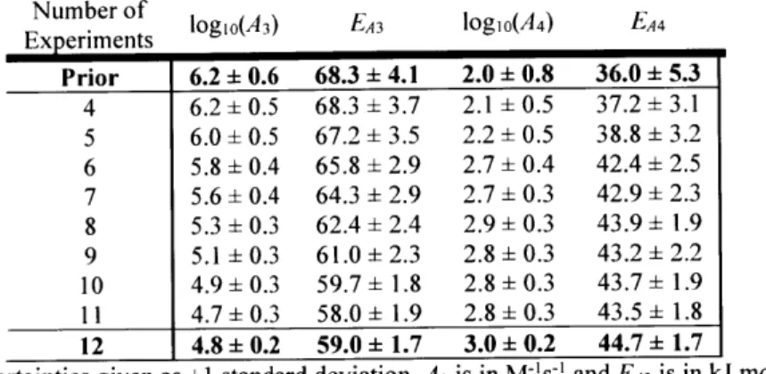
Table 2.4. Optimal kinetic parameter estimates from isolated estimation and uncertainties* of parameters A3 and EA3 and parameters A4 and EA4... 63
Table 2.5. Optimal kinetic parameter estimates and uncertainties from final simultaneous experim ent in isolated approach ... 64
Table 3.1. Slug experimental conditions for 2,4-dichloropyrimidine-morpholine reaction test of carry ov er... 89
Table 4.1. Simulated catalyst-specific activation energy correction factors (Ei) in kJ mol-1.... I 10 Table 4.2. Optimization results for y = 0.90. Nexpts = 83 23... 111
Table 4.3. Optimization results for y = 0.95. Nexpts = 66 6... 112
Table 4.4. Optimization results for y = 0.98. Nexpts = 74 12... 112
Table 4.5. Optimization results for y = 0.90. Nexpts = 116 39... 115
Table 4.6. Optimization results for y = 0.95. Nexpis = 76 13... 115
Table 4.7. Optimization results for parallel reactions A + B 4 R and B 4 Si. Nexpts = 66 5. 117 Table 4.8. Optimization results for series reactions A + B 4 R and B + R 4 S2. Nexpts = 65 6. ... 1 18 Table 4.9. Optimization results for case of catalyst I deactivation at T > 80'C. Nexpts = 151 83. ... 12 0 Table 4.10. Optimization results for case of catalyst I deactivation at T > 80'C, assuming a trust region on the calculation of the prediction covariance of i of 0.9 min tres, 8'C T, and 0.33 m M Ccal. Nexpts = 140 73. ... 122
Table 4.11. Optimization results for case of catalyst I deactivation at T > 80'C, assuming a trust region on the calculation of the prediction covariance of i of 0.22 min tres, 20C T, and 0.08 m M Cc at. Nexps = 136 33. ... 122
Table 5.1. Observed maxima and maxima predicted by a linear response surface model through 40 fractional factorial design experiments. Dashed border represents solvents below m inim um yield tolerance... 132 Table 5.2. Observed maxima and maxima predicted by a linear response surface model through 67 fractional factorial and sequential RSM experiments. Dashed border represents solvents below m inim um yield tolerance. ... 134 Table 6.1 Optimal yield and TON found by automated optimization of Suzuki-Miyaura case studies. Yields for syntheses of 10, 15, and 19 are based on conversion of the aryl h a lid e ... 15 0 Table 6.2. Optimal TON conditions for the reaction of 9 and 7 to produce 10. P1-L1 was found to be optim al in 97 experim ents... ... ... 151 Table 8.1. Table of Latin nom enclature... 161 Table 8.2. Table of G reek nom enclature. ... 163 Table Al. List of experimental conditions and measured outlet concentrations for initial sim ultaneous param eter estim ation... 185 Table A2. List of experimental conditions and measured outlet concentrations for isolated estim ation of A i, EAi, A2, and EA2. ... 185 Table A3. List of experimental conditions and measured outlet concentrations for isolated estim ation ofA 3 and EA3. ... 1 86
Table A4. List of experimental conditions and measured outlet concentrations for isolated estim ation of A 4 and EA4. ... 186
Table A5. List of experimental conditions and measured outlet concentrations for final sim ultaneous param eter estim ation... 187 Table C. 1. Predicted optimal conditions and TON for kinetics of Case Study I with y = 0.90. 236 Table C.2. Predicted optimal conditions and TON for kinetics of Case Study I with y = 0.95. 238 Table C.3. Predicted optimal conditions and TON for kinetics of Case Study I with y = 0.98. 241 Table C.4. Predicted optimal conditions and TON for kinetics of Case Study 2 with y = 0.90. 243 Table C.5. Predicted optimal conditions and TON for kinetics of Case Study 2 with y = 0.95. 246 Table C.6. Predicted optimal conditions and TON for kinetics of Case Study 3 with competing reaction B -> S i. ... 24 8
Table C.7. Predicted optimal conditions and TON for kinetics of Case Study 3 with competing
reaction B + R 4S2 ... ... 251
Table C.8. Predicted optimal conditions and TON for kinetics of Case Study 4 with no prediction covariance trust region...253
Table C.9. Predicted optimal conditions and TON for kinetics of Case Study 4 with 10% prediction covariance trust region. ... 256
Table C.10. Predicted optimal conditions and TON for kinetics of Case Study 4 with 2.5% prediction covariance trust region. ... 258
Table D. 1. Observed yields for conditions screened during first fractional factorial design. .... 261
Table D.2. Observed yields for conditions screened during second fractional factorial design. 262 Table D.3. Observed yields for conditions screened during response surface optimization with G-optim al design of experim ents criterion. ... 263
Table D.4. Observed yields for conditions screened during quasi-Newton gradient-based search. ...- ...---... 264
Table E. 1. Experimental data for reaction optimization of 13 and 14. Yields based on conversion of 13... ....---... 266
Table E.2. Optimal yield and TON conditions for optimization of 13 and 14. Yields based on conversion of 13. ... ... . - - -... 269
Table E.3. Experimental data for reaction optimization of 16 and 14... 270
Table E.4. Optimal yield and TON conditions for optimization of 16 and 14. ... 272
Table E.5. Experimental data for reaction optimization of 16 and 18. Yields based on conversion of 16... ...- - - - --... 273
Table E.6. Optimal yield and TON conditions for optimization of 16 and 18. Yields based on conversion of 16. ... ---- ... 275
Table E.7. Experimental data for reaction optimization of 9 and 7. Yields based on conversion of 9. ...--- --- --- ---... 276
Table E.8. Optimal yield and TON conditions for optimization of 9 and 7. Yields based on conversion of 9. ...- - -- - - -- .... 278
Table E.9. Experimental data for screening of 9 and 7. Yields based on conversion of 9... 279
Table E. 10. Experimental data for reaction optimization of 16 and 20... 280
LIST OF SCHEMES
Scheme 1.1. Heck reaction optimization studied by McMullen et al.22 ... . . . .. .. . . 32
Scheme 1.2. The methylation of primary alcohols by DMC in supercritical C02 studied by P arrott et a l.84 . ... 33 Scheme 1.3. Hydrogenation optimization studied by Fabry et al... . . . .. . . 35 Scheme 1.4. Optimization of imine formation by inline NMR from Sans et al.61 ... 35 Scheme 1.5. Paul-Knorr reaction optimization studied by Moore and Jensen.s5 ... 36 Scheme 1.6. Diels-Alder reaction used in the kinetic study by McMullen and Jensen. 23... 37
Scheme 2.1. Multi-step reaction network for conversion of 2,4-dichloropyrimidine to 4,4'-(2,4-pyrim idinediyl)bis-m orpholine... 42 Scheme 2.2. Reaction of 2,4-dichloropyrimidine and morpholine... 59 Scheme 2.3. Reaction of 4-(2-chloro-4-pyrimidinyl)-morpholine and morpholine. ... 59 Scheme 2.4. Reaction of 4-(4-chloro-2-pyrimidinyl)-morpholine and morpholine... 59 Scheme 3.1. Suzuki-Miyaura cross-coupling of 2-chlorobenzoxazole and I -boc-2-pyrroleboronic acid catalyzed by XPhos-OMs precatalyst. ... 91 Scheme 3.2. Suzuki-Miyaura cross-coupling of 2-chloropyridine and 1 -boc-2-pyrroleboronic acid catalyzed by XPhos-OMs precatalyst. ... 92 Scheme 5.1. Optimization conditions for the mono-alkylation of trans-1,2-diaminocyclohexane.
... 12 7 Scheme 5.2. Mono-alkylation of (JR,2R)-(-)-1,2-diaminocyclohexane... 134 Scheme 6.1. Optimization scheme for Suzuki-Miyaura cross-couplings in the presence of DBU and T H F/W ater. ... 140 Scheme 6.2. Optimum for the Suzuki-Miyaura cross-coupling of 3-bromoquinoline and 3,5-dimethylisoxazole-4-boronic acid pinacol ester... 144 Scheme 6.3. Optimum for the Suzuki-Miyaura cross-coupling of 3-chloropyridine and 3,5-dimethylisoxazole-4-boronic acid pinacol ester... 145 Scheme 6.4. Optimum for the Suzuki-Miyaura cross-coupling of 3-chloropyridine and benzofuran-2-boronic acid... 146 Scheme 6.5. Optimum for the Suzuki-Miyaura cross-coupling of 2-chloropyridine and I -boc-2-pyrroleboronic acid... 147
Scheme 6.6. Optimum for the Suzuki-Miyaura cross-coupling of 3-chloropyridine and 3,5-dim ethylisoxazole-4-boronic acid. ... 148 Scheme 6.7. Suzuki-Miyaura cross-coupling of 3-chloropyridine and benzofuran-2-boronic acid p in aco l ester... 152
1. FEEDBACK SYSTEMS FOR THE ACCELERATION OF REACTION DEVELOPMENT
With the cost to discover and develop a drug now estimated to exceed $2 billion,' the pharmaceutical industry is in search of innovative and cost-effective ways to reduce process footprint, minimize lead times, and accelerate scale-up. One path to achieving these goals that has received great attention lately is the adoption of continuous flow technology.2-4 In the past few years, the pharmaceutical industry has begun to incorporate continuous processing into more and more small molecule syntheses, with applications ranging from the replacement of individual batch unit operations for safer,5-8 greener,9-12 and/or more aggressive flow reaction steps,13-16 to the design and implementation of an end-to-end pilot plant encompassing continuous drug manufacture.'7 It is widely accepted that the continued introduction of efficient and rapidly scalable technologies for the acceleration of reaction development into manufacturing will help greatly in delivering drugs in less time and at lower cost to the patient.
A breadth of technologies and methodologies fall under the heading of "acceleration of reaction development." Much of our lab's focus has been in the development of microreaction technology,]8-21 namely the use of sub-millimeter scale reactors to achieve highly controlled chemical syntheses that can then be scaled to larger flow systems.22-25 This is made possible by the excellent rates of heat and mass transfer26 and minimal dispersion27 in microscale systems, which enable easier access to the intrinsic kinetics of the reaction.23,28-31 The reduced volumes of microreactors further allow profiling of reactions at conditions that would be too hazardous or simply impossible to achieve in batch, a few examples of these being reactions of azides,, 32 fluorinations,3 3 3 6 nitrations,3 7 3 8 DIBAL-H reductions,3 94' lithiations, 39,42-4 Grignard reactions,39,42,46,47 and reactions in supercritical media.48-50 Data collection from continuous flow
systems is accelerated by the incorporation of online analytics such as HPLC ,22,23,30,51 MS,52,5 3 GC,28 UV-Vis,14 55 FTIR,2 8,56-59 Raman,60 and NMR.61 These instruments allow the experimenter
near infinite access to the inner workings of the chemistry, enhancing understanding of reaction mechanisms, formation rates of intermediates and byproducts, and responses to perturbations in process conditions.
Of course, to some "acceleration of reaction development" does not only imply easier scalability, but actually running more experiments in a reduced period of time. This is the essence of high-throughput experimentation (HTE),6 2 66 whereby automation and robotics are
used to rapidly conduct and analyze many experiments in parallel with little to no intervention required on the part of the scientist. These tools enable fast understanding of the reaction performance as a function of many different variables, with full reaction maps being assembled in time spans of days down to a few hours.67-6 8 By minimizing the volume of each reaction sample, reaction profiling can be completed with milligram-scale quantities of expensive pharmaceutical precursers63 or nanogram-scale quantities of expensive catalysts or ligands. Yet techniques imported from high-throughput drug discovery are often limited in scope, ranging from the limited scalability of batch results to limitations in the ability to modulate key factors such as reaction time or temperature. To alleviate these concerns, efforts have been made to employ rapid automated experimentation in flow, merging the scalability of microreaction technology with the sheer sneed of HTF. 22,34,37
Unfortunately, the direct assimilation of HTE and automation approaches into chemical synthesis introduces a new problem-the curse of dimensionality. To illustrate, consider a case study where an experimenter is interested in studying the combined effects of 10 catalysts and 10 ligands. Teasing out all of the catalyst-ligand interactions would require 100 experiments, which can be easily executed in a single parallelized screen. Now consider the addition of 10 solvents and 10 bases to the study, giving 10,000 total experiments to be run. While such a system is still solvable, the cost of these experiments is substantially more. What if the kinetics of the reaction are important, such that the experimenter needs to also study 10 temperatures and 10 reaction times? Alternatively, how much money and time are lost in screening if one of these variables is found later to have no effect on the reaction? Clearly simplifications are needed and often employed, the most well-known of these being the one-factor-at-a-time approach.6 9 Yet by manipulating only a single variable at a time, then optimizing, then moving to a new variable, all of the information is lost from the system with regard to how multiple variables interact with one another, which can be critical when constructing reaction mechanisms or identifying an optimal process envelope. It is also easy to see that such an approach can lead to identification of less-than-optimal process conditions, leading to reduced yields in scale-up, or the worst-case possibility of not being able to manufacture the drug altogether.
A better approach that addresses the concerns listed above is to use feedback to engineer reactions to more optimal conditions. Unlike straight HTE, all experimental conditions are not screened upfront; rather one or multiple initial experiments are chosen as an initialization, then
an optimization routine selects the next best experiment or set of experiments to run that moves the system toward finding an optimum (Figure 1.1). To accomplish this task, the optimization routine must first assess the fitness of previous experimental data points against an objective function. For deterministic routines, the data are then extrapolated to a model, which can be as simple as a piecewise response surface or as complex as to fully describe the kinetics and transport phenomena taking place within the system. Based upon this model, a more optimal experiment is selected, observed, and then the model is updated in iteration until convergence is reached.
Run Initial
Experimental Design
X3
Run New Experiment to
Move toward Optimum
x3
X3
X, OX*
Analyze Data and Fit
to Model or Response Surface
.9
Select New, More Optimal
Experiment to Run
A-1
I
min,, [Objective]
Figure 1.1 Generalized feedback loop for (deterministic) automated reaction optimization.
Naturally such an approach would be rather tedious in small-scale reaction development, hence the reason feedback optimal design has generally been reserved for instances where
experimental data are expensive to collect.70-74 With automation, however, the amount of user
interface required to collect a data point becomes considerably less. With the use of continuous flow and online analytics, smart automated systems can be constructed that use experimental data collected in real-time as feedback for rapid reaction development. In the simplest case, an automated feedback system can be used to identify the optimal yield for a reaction, but algorithms can also be constructed that identify best-fit reaction kinetics and mechanisms using information theory. In more complex reaction cases, questions arise as to the best way to
elucidate reaction kinetics in a single flow system, and how to optimize reactions in which discrete variables-such as catalysts, ligands, or solvents-interact differently with continuous variables-such as temperature, reaction time, or concentration. This thesis aims to answer both of these questions, and in so doing looks for a faster, more versatile, and more economical way to accelerate reaction development.
1.1.
THE TOOLS FOR FEEDBACK OPTIMIZATION IN FLOWThe general tools for flow chemistry have been reviewed recently.2' These comprise reagent
delivery, reaction, separation, analysis, and pressure control. Figure 1.2 illustrates how all of these components can be integrated into a single continuous flow feedback system. Both reagent delivery and reaction control (temperatures and flow rates) are controlled with a central automation software. Automation software and hardware can also be used to interface with online analytical devices that may identify changes in the process (for instance disturbances in temperature or pressure) or be used to extract quantitative data from the reaction-most often yields and conversion. These data are then passed to an optimization algorithm that interprets the data-perhaps also in the context of prior experiments-and use the information to project a new set of inputs that will move the system toward the optimum of a user-defined objective. These inputs are passed to the central control system, which makes the necessary manipulations to the experiment.
Central Control System
r -- -- - -- -- - i --- - - -- - - - - -- - - - - - - - -I- - - - - - - -
-Reagent Flow Separation Online Pressure
Delivery Reactor (if Necessary) Analysis Regulation Real-time
Optimization Algorithm
--- I
Figure 1.2. Block diagram for automated feedback optimization in flow systems.
For reagent delivery in optimization systems, our lab has had the most success using syringe pumps. These tend to produce the greatest accuracy in the flow rate range of I IL/min-250 pL/min, which depending on the number of pumps and size of reactor in use may translate to
residence times of 30 s to 30 min. At or below 30 s, the rate of mixing can become a key confounding variable in the optimization.27 Reaction times of 30 min or more are usually undesirable for rapid feedback because the time to reach steady-state in continuous, non-droplet, systems is greater than or equal to triple the residence time. Long reaction times may be more suitable for flow rate ramps, where each segment of fluid is treated as a separate batch reactor.29 For accurate optimization results, the choice of syringe material can matter greatly. Despite their convenience and low cost, plastic syringes are almost never desirable because of the tendency of the plastic plungers and barrels to buckle and produce inconsistent flow rates under even the mildest of pressures. Glass syringes are excellent in terms of accuracy and chemical compatibility; however these leak and therefore cannot be used at pressures above -14 bar. Even prolonged use at -7 bar will after several days require replacement of the syringe because of leaking. At high pressures, the only suitable syringe material option is stainless steel; however reagents which corrode stainless steel must be avoided.
Flow optimization systems require special treatment in reactor selection, as the nature of the experiment requires the reaction to proceed uninterrupted under a diverse and often sub-optimal range of experimental conditions. Flow reactors that are slow to reach temperature or cool down-most notably stainless steel or Teflon tubes submerged in an oil bath-tend to be undesirable for optimizations where the temperature must be manipulated regularly. Of course chemical compatibility with harsh organic reagents is of utmost concern, hence the avoidance of
PDMS in flow chemistry. Our lab's preferred reactor material has been silicon because of its excellent heat transfer properties and well-known microfabrication procedures, with the only notable limitation being its incompatibility with strong bases such as NaOH or KOH. For greater chemical compatibility, glass75,76 or silicon carbide77 reactors are available, though these are
more difficult to machine and are expensive to replace in the event of a clog. In this thesis, a new reactor is introduced which comprises a Teflon tube heated in an aluminum chuck. The advantages of this design are extensive chemical compatibility, easy replacement of the Teflon tube in the event of temperature-induced degradation or clogging, and faster equilibration to the set point temperature compared to heating in an oil bath.
The available tools for online analysis were discussed earlier, and any and all could be applied to flow optimization systems. Our lab has explored predominantly online HPLC-because of its ability to resolve a diverse spectrum of reaction products-and FTIR-because of the speed at
which data can be collected and fed back to the process. The time needed to collect data by HPLC makes LC analysis the limiting step in many instances of feedback optimization. Consequently, work has been done in recent years to improve the speed of HPLC analysis for high-throughput applications.7 8 7 9
As is always the concern, the greater the specificity in designing an optimal LC method for a given reaction, the less generalizable the platform can be for broader scopes of substrates and products.
The design of an optimization system with automation software is dependent upon recognizing which variables are to be controlled and which observables (responses) are to be measured. As straightforward as it may seem, model inputs that cannot be controlled cannot be manipulated to achieve an optimum. Likewise outputs that cannot be measured cannot be optimized, unless there is a model relating another measured output to the desired response. Inputs can be controlled by local controllers (for instance most syringe pumps deliver at a controlled flow rate once a set point is received) or by the central controller. The choice of when to use either is usually a matter of how much control needs to be exercised and what local controllers, if any, are available (for example if the pump flow rate needs to change as a function of pressure but the pump has no pressure sensor, then this loop is built into the central controller). Sometimes sensory measurements trigger decisions by the control system, such as the decision to switch valves and flush out a reactor on account of an observed increase in pressure.80
Constraints with regard to maximum and minimum values of the controlled inputs are almost always incorporated into the optimization and control routine and depend upon the physics of the system. For sake of clarity in the subsequent sections and chapters, the responses are the measurements that factors into the objective of the optimization-for instance product yield, which is estimated based on a calibration model of the measured analytical signal. In all of the accounts presented herein, LabView (National Instruments Corporation) was used as the central control software for manipulating inputs. Responses were sometimes interpreted directly by LabView, or worked up analyses were passed to LabView from software such as ChemStation (Agilent Technologies) or iC IR (Mettler Toledo International Inc.). Optimization routines executed in MATLAB (The MathWorks Inc.) or LabView provided new set points for
1.2. REACTION OPTIMIZATION "FROM SCRATCH"
With no prior information or models to which to resort, a plausible optimization strategy must accept input factors known to influence the desired response and interpret relationships among these variables which lead to improvement-and hopefully optimality-in an objective. Such a model-free strategy is commonly referred to as "black box" optimization. An important aspect of black box optimization is that, from an engineering standpoint, little to no modeling information
is gained from the search. Consequently, optimal results have no guarantee to transfer across scales. This is of course the major concern of using black box approaches for the application of reaction development, where the ultimate goal is scale-up. However, if the feedback system is engineered to detect intrinsic reaction rates, the results of black box optimization routines can still have great utility, especially when little to no a priori information is known about the chemistry. If optimization of the flow system is desired simply to increase production rate or yield in the same flow reactor, black box strategies are excellent simple tools to identify improved or perhaps optimal reaction conditions.
Some of the earliest methods for incorporating black box optimization algorithms into automated microreactor experiments were developed by Krishnadasan et al.8 1 and by McMullen and Jensen.2 2 Krishnadasan et al. employed a Stable Noisy Optimization by Branch and Fit (SNOBFIT)82 algorithm to optimize the automated synthesis of CdSe quantum dots. Nanoparticles were monitored inline by fluorescent emission measurements from a CCD spectrometer, and a feedback loop allowed for tuning of the microreactor temperature and flow rates in order to maximize the quantum dot emission at a specified wavelength. McMullen and Jensen compared the SNOBFIT algorithm with two local-search black box optimization algorithms-Nelder-Mead Simplex and steepest descent-in studying the Knoevenagel condensation reaction of p-anisaldehyde and malononitrile. Species concentrations were monitored online by HPLC. The two-dimensional optimization of reactor residence time and temperature consistently identified the maximum objective function value as occurring at the maximum allowable reaction temperature of 1000C and the minimum residence time of 30 min, regardless of the optimization method employed. The fastest convergence upon the optimum was achieved with the gradient-based steepest descent method.
Though only a local search strategy, the Simplex method83 has been used extensively in black box flow optimization systems. In its simplest implementation, Simplex selects k+ 1 points for a
k-dimensional optimization, then after identifying the least optimal point from that experimental set, reflects the least optimal point across the polygon defined by the other k points to define a new Simplex. When no improvement in the optimization is achieved, the size of the Simplex is reduced and the method repeats. This strategy is both simple to implement and does not require approximation of a gradient, which caters well to expensive experimentation. In one application, McMullen and Jensen demonstrated use of the Simplex method in a four-dimensional optimization of benzaldehyde production, increasing the yield from 21% to 80%.1' The Simplex method was further applied in optimizing the number of alkene equivalents and reaction time in a selective Heck reaction (Scheme 1.1).22 In both cases, syringe pumps were connected to a temperature-controlled silicon microreactor, with analysis performed by online HPLC (Figure
1.3). The feedback optimization algorithm was executed in MATLAB and the system was
controlled with LabView software. For the Heck reaction example, nine sets of reaction conditions were then scaled 50 times to a 7 mL Coming Advanced-Flow glass reactor module. The scaled optimum was found to be consistent with the microscale optimum and resulted in the synthesis of 26.9 g desired product at 80% yield.
1 mol% Pd(OAc)2
CI 3 moI%L P.-. CF
3 F3C F
F3C C \ 1.2 equiv. y2NMe C/F3 CF3
n-butanol, 900C
Equiv = 1.0-6.0 tres = 3.0-8.0 min Desired Undesired
PBu2
L = Me
Scheme 1.1. Heck reaction optimization studied by McMullen et al.22
Micoreactor A B TewperatuL Canr"l Reaction Flow-Rale Anayss contrd kd
Poliakoff and coworkers84-8 8 have been interested in the use of feedback for online optimization of the methylation of primary alcohols by dimethyl carbonate (DMC) in supercritical C02 (Scheme 1.2). Here the advantage of the flow system was both in rapid optimization and in the accessibility of supercritical reaction conditions. In the original system, Parrott et al.84 flowed the methylation reactants through a packed bed of y-alumina in the presence of supercritical C02 and monitored the reaction yield by online GC. The Super Modified Simplex algorithm89 was used to optimize the reaction yield with respect to temperature, pressure, and the flow rate of C02. The Super Modified Simplex algorithm functions similarly to Nelder-Mead Simplex but additionally determines if the size of the Simplex can be expanded in regions of the experimental space where little change in the objective is observed-hence leading to faster convergence. Even with the improved convergence rate, approximately 35 hr were required for the optimizations in the study. Improvements to the system were later made by Bourne et al.85 (who included equivalents of methylating agent as a variable in the optimization), Jumbam et al.86 (who demonstrated optimization over several objective functions including yield, space-time yield, and E-factor), and Skilton et al.87 (who accelerated data collection with use of an FTIR and compared the performance of Simplex to SNOBFIT). Most recently the group demonstrated the potential of automated chemical reaction systems by allowing a researcher to remotely study and optimize the UK-based system from Brazil.8 8
DMC 0
HO R y-alumina O2R _O R
T?
R = H, C2H7 P?
CO2 Flow Rate?
Control Feedback Monitor --- v- Control -. I Software
'Reactants
CO
2 - - - -e-S GC - - - - BPR - ----Products
Figure 1.4. Automated system for optimization of the methylation of alcohols introduced by Parrott et al.14
M is a static mixed and R is the reactor packed with catalyst.
Recent applications of automated optimization systems have demonstrated incorporation of more advanced synthesis and analytical systems into the Simplex algorithm framework. In increasing the scope of chemistries available for feedback control, the utility of smart optimization systems has increased substantially. As an example, Fabry et al.90 coupled LabView
software to a commercial flow hydrogenation system, the H-cube, and demonstrated optimization of Scheme 1.3 with respect to hydrogen pressure, temperature, and flow rate. Inline FTIR was used for analysis. The Simplex optimization required 24 hr to complete 17 experiments but identified optimal conditions for 99% conversion to the alcohol product. Feedback optimization with an inline NMR, introduced by Sans et al.,61 offers the researcher an opportunity to study kinetics of intermediate formation and optimize chemistries that would be otherwise impossible to observe by optical or chromatographic techniques. In an application of Nelder-Mead Simplex, Sans et al. optimized imine formation in the reaction of 4-fluorobenzaldehyde and aniline (Scheme 1.4) by monitoring reaction yield and conversion with 'H NMR. The optimization resulted in a reduction of reaction time to 2 min, while the reaction
yield was maintained above 70%. It is inevitable that to study more complex chemistries inline, multiple analytical instruments such as IRs, LCs, GCs, and/or NMRs will be incorporated into flow systems in series or in parallel to maximize the information gained on a per experiment basis. 0 5 wt% Pd/C OH R H2 =0-100 bar R T = 20-100OC R = H, COOEt, CH2COOEt 0.1 M Flow = 0.3-1.0 ml/min
Scheme 1.3. Hydrogenation optimization studied by Fabry et al.9 0
0 0.05 M TFA
S H ~N H 2 MeCN
F H + NH tres = 2-10 min F N
CAO =0-0-1.0 M CBO = 2.0 M - 2*CAO
Scheme 1.4. Optimization of imine formation by inline NMR from Sans et al.61
Despite the popularity of the method, the Simplex optimization routine can struggle to converge efficiently on account of the algorithm chosen for Simplex contraction, the dimensionality of the optimization, and the initial guess. Gradient-based optimization strategies tend to offer much faster convergence rates, at the expense of the extra experiments involved in gradient calculation. With a slow HPLC method, for instance, the time required for a gradient estimation can be quite limiting, but with the emergence of technology such as inline FTIR the use of gradient-based optimization methods should become more widely accepted. As an example of the speed at which feedback optimization can be accomplished with a gradient search, Moore and Jensen 8 demonstrated optimization of space-time yield for a Paul-Knorr reaction (Scheme 1.5) with three different gradient-based searches: steepest descent, conjugate gradient, and conjugate gradient with an Armijo step size. As illustrated in Figure 1.5, the rate of convergence effectively doubled when the conjugate gradient method was used compared to the
steepest descent method, because of the additional gradient history incorporated into the selection of the conjugate gradient search direction. With a smarter selection of step size (following the Armijo rule91), the rate of convergence of the same optimization was accelerated to greater than three times the rate of convergence of the original steepest descent method. Though these methods are still black box local optimization searches, their abilities to rapidly
map out the trajectory to an optimum allow experimenters a quantitative interpretation of the response surface curvature that could be of service to kinetic investigations.
0
+ H2N OH DMSO 0- N
o T = 30-130C OH
tres = 2-30 min
Scheme 1.5. Paul-Knorr reaction optimization studied by Moore and Jensen.5
0.10 0.09 -0 90 a.0 00 0 0 0 0 A 00o 0 0 3 0 04 0 A 0f 0.03-0.01 0 20 40 6 80 100 120 140 Setpaint Number
Figure 1.5. Convergence of the PauI-Knorr reaction from the automated system of Moore and Jensen.58
Diamond-steepest descent algorithm. Circle-conjugate gradient algorithm with fixed step size.
Triangle-conjugate gradient algorithm with Armijo step size.
1.3. KINETICS IN FLOW: A ROUTE TO FASTER SCALE-UP
Though black box strategies are valuable tools for identifying improved reaction conditions in less time than combinatorial or one-factor-at-a-time screening, predictable scalability of results can only come from a complete understanding of the reaction mechanism and kinetics. Identification of reaction kinetics in flow offers many of the advantages already discussed in previous sections in terms of fast heat and mass transfer rates and more precise control of reaction conditions. Additionally, with feedback an automated system can determine which kinetic experiments are most valuable to run in order to select optimal rate parameters and an optimal rate law. This offers an invaluable tool to the experimenter looking to discriminate among many possible reaction mechanisms.
As an example of using feedback in the determination of reaction kinetics, McMullen and Jensen2- used a silicon microreactor flow system with online HPLC sampling to study the