Marginal Abatement Cost Curves and Quality of Emission Reductions: A Case Study on Brazil

HAL Id: hal-00966821

https://hal-enpc.archives-ouvertes.fr/hal-00966821v3

Submitted on 30 Oct 2014

HAL is a multi-disciplinary open access

archive for the deposit and dissemination of

sci-entific research documents, whether they are

pub-lished or not. The documents may come from

teaching and research institutions in France or

abroad, or from public or private research centers.

L’archive ouverte pluridisciplinaire HAL, est

destinée au dépôt et à la diffusion de documents

scientifiques de niveau recherche, publiés ou non,

émanant des établissements d’enseignement et de

recherche français ou étrangers, des laboratoires

publics ou privés.

Emission Reductions: A Case Study on Brazil

Adrien Vogt-Schilb, Stéphane Hallegatte, Christophe de Gouvello

To cite this version:

Adrien Vogt-Schilb, Stéphane Hallegatte, Christophe de Gouvello. Marginal Abatement Cost Curves

and Quality of Emission Reductions: A Case Study on Brazil. Climate Policy, Taylor & Francis, 2014,

pp.15. �10.1080/14693062.2014.953908�. �hal-00966821v3�

A Case Study on Brazil

Adrien Vogt-Schilb1,2,∗_{, St´ephane Hallegatte}1_{, Christophe de Gouvello}3

1_{The World Bank, Climate Change Group, Washington D.C., USA} 2_{CIRED, Nogent-sur-Marne, France}

3_{The World Bank, Energy and Extractive Global Practice, Brasilia, Brazil}

Abstract

Decision makers facing emission-reduction targets need to decide which abatement measures to implement, and in which order. This paper investigates how marginal abatement cost (MAC) curves can inform such a decision. We re-analyse a MAC curve built for Brazil by 2030, and show that misinterpreting MAC curves as abatement supply curves can lead to suboptimal strategies. It would lead to (i) under-investment in expensive, long-to-implement and large-potential options, such as clean transportation infrastructure, and (ii) over-investment in cheap but limited-potential options such as energy-efficiency improvement in refineries. To mitigate this issue, the paper proposes a new graphical representation of MAC curves that explicitly renders the time required to implement each measure.

Policy relevance

In addition to the cost and potential of available options, designing optimal short-term policies requires information on long-term targets (e.g., halving emissions by 2050) and on the speed at which measures can deliver emission reductions. Mitigation policies are thus best investigated in a dynamic framework, building on sector-scale pathways to long-term targets. Climate policies should seek both quantity and quality of abatement, by combining two approaches. A “synergy approach” that focuses on the cheapest mitigation options and maximizes co-benefits. And an “urgency approach” that starts from a long-term objective and works backward to identify actions that need to be implemented early. Accordingly, sector-specific policies may be used (i) to remove implementation barriers on negative- and low-cost options and (ii) to ensure short-term targets are met with abatement of sufficient quality, i.e. with sufficient investment in the long-to-implement options required to reach long-term targets.

Various options are available to reduce greenhouse gas (GHG) emissions: fuel switching in the power sector, re-newable power, electric vehicles, energy efficiency improve-ments in combustion engines, waste recycling, forest man-agement, etc. Policy makers have to compare and assess these different options to design a comprehensive miti-gation strategy and decide the scheduling of various ac-tions (i.e. decide what measures need to be introduced and when). This is especially true concerning the emission-reduction measures that require government action (e.g., energy-efficiency standards, public investment, public plan-ning).

Marginal abatement cost (MAC) curves are largely and increasingly used in the policy debate to compare miti-gation actions (Kesicki and Ekins, 2012; ESMAP, 2012;

Kolstad et al., 2014). A MAC curve provides information on abatement costs and abatement potentials for a set of mitigation measures. They can serve as powerful tools to

∗_{Corresponding author}

Email addresses: avogtschilb@worldbank.org (Adrien Vogt-Schilb), shallegatte@worldbank.org (St´ephane Hallegatte), cdegouvello@worldbank.org (Christophe de Gouvello)

communicate that large amounts of emission reductions are technically possible. They also show that some emis-sion reductions can pay for themselves due to co-benefits such as energy efficiency gains or positive impact on health, and that many others will be inexpensive (in terms of net present social value). This information can help govern-ments decide how ambitious their mitigation strategy will be, and make informed domestic and international com-mitments (in the UNFCCC context, for instance). It is also helpful for policy makers searching for synergies and co-benefits, for instance between emission reduction and economic development.

The academic literature on MAC curves has exten-sively discussed the plausibility of energy efficiency op-tions that would reduce emissions at net negative costs. In general, MAC curves do not factor in implementation barriers on these options, such as split incentives, lack of information, behavioral failures, or lack of resources ( All-cott and Greenstone,2012;Kesicki and Ekins,2012).1 Ac-cording to this literature, overcoming such barriers may be

1 _{The investor’s MAC curves commissioned by the EBRD are}

costly enough to reduce significantly the economic benefits from energy savings. To date, identifying specific barriers and cost-effective ways of working around them remains a policy-relevant challenge (e.g.,Giraudet and Houde,2013). The issue discussed here is different. Because they rank options according to their cost — from the least to the most expensive — MAC curves look like abatement supply curves (Fig.1), and are frequently interpreted as such (e.g.

Haab, 2007; DECC, 2011). According to this interpreta-tion, the optimal emission-reduction strategy would be to “implement the cheapest measure first, preferring measures with a lower total saving potential but more cost-effective than those with a higher GHG saving potential in absolute terms” (W¨achter, 2013). In this paper we show why this strategy is not the optimal one, we propose a new graphical representation of MAC curves that avoid this misinterpre-tation, and we derive broader policy implications on the design of climate mitigation strategies.

In addition to the cost and potential, a key param-eter of emission reduction options is the speed at which they can be implemented. Speed is limited by factors such as (1) long capital turnover, (2) slow technological dif-fusion, (3) availability of skilled workers, (4) availability of relevant specific capital, such as production lines, (5) availability of funds or (6) institutional constraints.2 As a consequence, some high-abatement-potential measures, such as switching to renewable power or retrofitting exist-ing energy-inefficient buildexist-ings, may take decades to im-plement. While the cost and potential displayed in a MAC curve are frequently assessed with such maximum speed in mind, the diffusion speed itself is almost never displayed in the MAC curve or generally disclosed to decision-makers. With a simple theoretical model,Ha-Duong et al.(1997) find that this technical inertia (using the wording byGrubb et al., 1995) means that the optimal quantity of short-term abatement depends on long-short-term objectives — an extensive literature based on integrated assessment models has reached the same conclusion (e.g.Luderer et al.,2013;

Bertram et al., 2014; Riahi et al.,2014). Using a theoret-ical MAC curve, Vogt-Schilb and Hallegatte (2014) show that the quality of abatement is also important. The au-thors argue short-term abatement targets should be reached with some of the high-potential but long to implement measures that will make deeper decarbonization possible in the long term, even if these are not the less expensive measures available in the short term. As a consequence, focusing on short-term targets (e.g., for 2030) without con-sidering longer-term objectives (e.g., for 2050 and beyond)

of capital that the private sector faces, and positive transaction costs in their assessment of the abatement cost of each option (NERA,

2011b,2012,2011a).

2 _{In this paper we assume implementation barriers make the}

im-plementation of measures slower, without affecting their cost. In economic theory, an alternative approach is to consider adjustment costs that capture a trade-off between implementing options quickly and implementing them at low cost (Vogt-Schilb et al.,2012;Lecuyer and Vogt-Schilb,2014).

Figure 1: A measure-explicit marginal abatement cost curve. The general appearance of the curve makes it easy to misinter-pret it as an abatement supply curve, leading to the misguided conclusion that the “abatement demand” X should be met with measures 1 to 4 only (possibly using the carbon price Y).

would lead to carbon-intensive lock-ins, making it much more expensive (and potentially impossible) to achieve the long-term objectives.3

In this paper, we apply Vogt-Schilb and Hallegatte’s method on a MAC curve built at the World Bank for studying low-carbon development in Brazil in the 2010-2030 period (de Gouvello,2010). Lack of data beyond 2030 does not allow us to investigate how using only the 2010-2030 MAC curve to design a mitigation strategy would lead to suboptimal choices in view of longer-term objec-tives (2050 and beyond). We can however investigate this problem by assuming that we want to achieve an objec-tive for 2030, and that we use the MAC curve to design a mitigation strategy for the 2010-2020 period only.

We find that a strategy for 2010-2020 that disregards the 2030 target under-invests in clean transportation in-frastructure such as metro and train; and over-invests in marginal, cheap but low-potential options, such as heat integration and other improvements in existing refineries. In other words, developing clean transportation infrastruc-ture in the short term is appealing only if the long-term abatement target is accounted for. In addition, we find that not developing clean transportation infrastructure in the short term (by 2020) closes the door to deeper emission reductions in the middle (2030) and longer term. Loosely speaking, the 2020 strategy provides a sensible quantity of abatement by 2020, but abatement is of insufficient qual-ity to reach the 2030 target. These results stress the need

3_{A related line of argumentation is on learning by doing and}

di-rected technical change (Gerlagh et al.,2009;Acemoglu et al.,2012;

Kalkuhl et al.,2012). Many of the technologies used to reduce emis-sions — for instance more efficient cars or renewable energy — are still in the early stage of their development, such that their cost will decrease as their deployment continues. Many authors have found in a variety of settings that this is a sound rationale to use expensive options in the short term (e.g.,Rosendahl,2004;del Rio Gonzalez,

2008; Azar and Sand´en, 2011). In the present work, we account for technical progress only to the (limited) extent that it can be cap-tured by the slow technological diffusion encompassed in our diffusion speed constraint.

for policymakers to take into account long term targets and the limited speed at which emission-reductions may be implemented when deciding on short-term action.

We derive two conclusions from this work.

First, MAC curves do not report a very important piece of information, namely the implementation pace of each measure and option. We suggest that when MAC curves are produced, they should be presented together with the corresponding emission reduction scenario — us-ing the graphical representation thatPacala and Socolow

(2004),Williams et al.(2012) andDavis et al.(2013) call wedge curves — making the dynamic aspect of the mitiga-tion scenarios more explicit (Fig.2). Note that this pro-posal concerns only the graphical communication of abate-ment measures, their impact on greenhouse gas emissions over time, and their cost; without any prescription on the method used to assess those numbers.

For instance, emission reduction potentials and costs are frequently assessed from expert surveys (e.g.ESMAP,

2012). MAC curves built this way would be greatly im-proved by an explicit discussion of implementation bar-riers and factors limiting the pace at which emission re-ductions may be achieved with each particular measure (seeAppendix Bfor suggested guidance for the experts in charge of collecting the information to build a MAC curve). This information would be particularly useful for decision makers if it permits identifying distinct bottlenecks (e.g. availability of skilled workers) that can be translated into specific policies (e.g. training).

Emission reduction scenarios, costs and potentials can also be derived from energy system models (Kesicki,2012b).4

These models account for the limited ability to implement emission-reduction measures by building in particular on maximum investment speeds (Wilson et al., 2013; Iyer et al., 2014), making them suitable for studying path de-pendency in emission reduction strategies (Kesicki,2012a). MAC curves built this way can also be presented next to the corresponding wedge curve, as in Fig.2. In this case also, the policy debate is improved by an explicit discus-sion of how the growth constraints are calibrated in the models (Wilson et al.,2013;Iyer et al.,2014).

Second, climate change mitigation policies are designed for a relatively short term horizon (e.g., 2020 or 2030), while mitigation objectives go beyond this horizon (e.g., the EU has a 2050 objective). Most importantly, sta-bilizing climate change and tackling other environmen-tal threats will require a reduction in emissions to near-zero levels by the end of the century (Collins et al.,2013;

Steinacher et al., 2013); following the wording by Sachs et al.(2014), any climate stabilization target requires deep decarbonization.

An ideal policy would be to announce well in advance

4 _{While existing MAC curves in the gray literature are mainly}

derived from expert surveys, the academic literature frequently stud-ies emission reduction pathways with energy system models or inte-grated assessment models.

a perfectly credible long-term target to a forward-looking market. In practice, however, governments have limited ability to commit, and markets cannot perfectly anticipate future regulations (Golombek et al.,2010;Brunner et al.,

2012). Following the World Bank(2012, p. 153), we thus suggest to combine a “synergy approach” focusing on mit-igation options that provide co-benefits in terms of devel-opment, economic growth, job creation, local environmen-tal quality, or poverty alleviation, with an “urgency ap-proach”, based on defining long-term objectives and work-ing backward to identify which measures are needed early to achieved stated objective.

Accordingly, sector-specific mitigation policies have two roles: (i) to remove implementation barriers on negative-and low-cost options, negative-and (ii) to ensure short-term targets are met without under-investing in the ambitious and long-to-implement abatement measures required to achieve other-wise-difficult-to-enforce long-term targets. In other words, these policies should ensure that the mitigation strategy reaches not only the desired quantity of abatement at a given date, but also a sufficient quality to make further emission reduction possible.

This second argument for sector-specific policies, in line withWaisman et al.(2012), remains a novelty in the aca-demic literature: to date, such policies have been discussed as a way to tackle several market failures or policy ob-jectives, including learning by doing (Sand´en and Azar,

2005;Fischer and Preonas,2010); to correct for the effects of misperceived energy savings (Tsvetanov and Segerson,

2013; Parry et al., 2014); to complement an imperfect carbon-pricing mechanism (Lecuyer and Quirion,2013); or as a political economy constraint (Hallegatte et al.,2013;

Jenkins,2014;Rozenberg et al., 2014).

The rest of the paper is structured as follows. In sec-tion1, we review different types of MAC curves. While the construction of MAC curves sometimes requires to in-vestigate the diffusion speed of emission-reduction options, MAC curves do not report separately the long-term abate-ment potential and the diffusion speed. In section2, we reanalyze the data from the Brazilian MAC curve. We ex-tract the cost, long-term potential and diffusion speed of each emission-reduction measure, and use them in a simple optimization model to investigate the least-cost emission-reduction schedule, depending on whether the objective is to reach a 2030 target or the corresponding 2020 target. We conclude in section3.

1. Existing MAC curves

We call measure-explicit MAC curves (MAC curves for short) these which represent abatement costs and poten-tials of a set of mitigation measures.5 _{Measure-explicit}

5 _{While the literature consistently calls these curves marginal}

abatement cost curves, in most occasions the cost of each option is computed as an average cost, as the net present cost of using that

Marginal cost

E

m

is

si

o

n

s

T

P

o

te

n

tia

l a

t

T

Wedge curve

Flipped MAC curve

Figure 2: A “flipped” achievable-potential MAC curves next to the corresponding emission reduction scenario (wedge curve). By displaying together the cost, the potential, and the time required to implement the options, confusion on how to interpret MAC curves may be avoided.

MAC curves have been developed since the early 1990s (Rubin et al.,1992), and have reached a wide public after McKinsey and Company published assessments of the cost of abatement potentials in the United States (McKinsey,

2007) and at the global scale (Enkvist et al.,2007). This type of curve is increasingly used to inform policy makers. For instance, McKinsey currently lists MAC curves for 15 different countries or regions on its website. The World Bank also uses MAC curves routinely (ESMAP, 2012), and has recently developed the MACTool to build them (see below). Similar depictions have been used by other institutions (e.g.,Climate Works Australia,2010;NERA,

2011a;CE Delft,2012;O’Brien et al.,2014) and to analyze other climate-change related topics, such as waste reduc-tion, energy savings and water savings (see Kesicki and Ekins,2012, who also offer a richer historical perspective). Depending on their implicit definition of the abatement potential of a measure, two types of measure-explicit MAC curves can be distinguished.

1.1. Full potential MAC curves

The full-potential approach gives information on how much GHG could be saved if the measure was used at its technical maximum. It is calculated against a reference or baseline technology, as for instance those used in the present (W¨achter, 2013), taking into account the carbon intensity and imperfect substitutability of different tech-nologies. For instance, this approach assesses what frac-tion of passenger vehicles can be replaced by electric vehi-cles (EV), accounting for limited driving range and exiting mobility practices. Given emissions from baseline vehicles

option instead of the baseline option, divided by discounted avoided emissions. Marginal and average costs are equal only if the unit cost of abatement is constant. Note that potentials spreading over large range of abatement costs may be split into smaller potentials of nearly constant abatement cost (Kesicki,2012b), for instance re-porting gas for base load and gas for peak power separately.

(e.g. 140g/km today in Europe) and emissions from EVs (say 30g/km), one can compute an amount of emissions avoidable using electric vehicles. Rubin et al. (1992) use this approach. For instance, they assess the potential of nuclear power (in the US) as the quantity of GHG that would be saved if nuclear replaced all the fossil fuel capac-ity used for base load and intermediate load operation in 1989.

The main value of full potential MAC curves is descrip-tive: they highlight to which extent some key measures could reduce emissions in the long-run. One weakness is that full-potential MAC curves cannot easily represent the competition between two measures.6 _{Finally, full-potential}

MAC curves do not require investigation of possible diffu-sion constraints, but these may be assessed separately to build resulting emission reduction scenarios (e.g. World Bank,2013).

1.2. Achievable potential MAC curves

Achievable-potential MAC curves have a prospective dimension, as they are built for a date in the future. This approach fully acknowledges that large-scale diffusion of new technologies can take decades (Gr¨ubler and Messner,

1998; Gr¨ubler et al., 1999; Wilson et al., 2013). In this context, the abating potential of a technology is an as-sessment of the abatement that could be achieved with such a technology if it was implemented at a given speed, starting at a given date. For instance, this approach takes into account that even ambitious fiscal incentives in fa-vor of electric vehicles would induce a limited increase of

6_{For instance, if fuel-cell vehicles are much more expensive than}

EVs, but do not suffer from limited autonomy, the optimal strategy would be to use EVs when possible (say for 25% of the fleet), and fuel cell vehicles otherwise. In this case, the full-potential MAC curve could depict an abatement potential of 25% of private-mobility related emissions for EVs, and 75% for fuel cell. In the absence of EVs, fuel cell vehicles could abate 100% of private mobility emissions, but this information would not appear in the curve.

EV sales, resulting in a limited share of EVs in the fleet, hence limited emission reductions from EVs by 2020 or 2030. The potential achievable by a given date is there-fore lower or equal than the full potential reported on full potential MAC curves.

A key advantage of the achievable-potential approach is that it requires investigation of reasonable assumptions regarding the possible implementation speed of a measure (e.g. 1% of the dwellings can be retrofitted each year). This information is key for a policy maker scheduling emission-reduction investments. Unfortunately, assessed diffusion speeds are not displayed in the resulting MAC curve, and are not always discussed in the accompanying reports.

Most expert-based MAC curves published in the gray literature are constructed this way — see for instance McK-insey(2009, p. 46), orPellerin et al.(2013, p. 22). The few curves built using integrated assessment models are also achievable-potential MAC curves (Kesicki,2012b). Achievable-potential MAC curves are built from emission-reduction pathways (Fig.2), that are investigated taking into account at least some inter-temporal dynamics and sector-specific constraints. It is thus logically inconsis-tent to conclude from an achievable-poinconsis-tential MAC curve that emission-reduction should be implemented sequen-tially in the “merit order”, cheapest first. The original emission-reduction pathways already provides an answer to when and where to reduce GHG emissions. Unfortu-nately, achievable-potential MAC curves have been fre-quently used overlooking their caveats, in particular in the media and policy debate (Haab,2007;Kesicki and Ekins,

2012).

One weakness of the achievable potential is that it makes the slow diffusion process indistinguishable from the full potential. The reader of a MAC curve does not know, for instance, if a small potential for abatement from res-idential building retrofit means that resres-idential buildings are already almost entirely retrofitted in the region (the full potential is low), or it if means that only a small frac-tion of buildings may be retrofitted during the period (the diffusion is slow).

The MAC curve we reanalyze in this paper is an achievable-potential MAC curve. In each economic sector, emis-sion reduction scenarios have been assessed taking into account constraints on implementation and maximum dif-fusion speeds (de Gouvello,2010).

1.3. MAC curves at the World Bank: MACTool

The World Bank develops and promotes a piece of software called MACTool, which can produce achievable-potential MAC curves. One aim of the MACtool is to pro-vide policy makers with a common framework to analyze available mitigation measures. MACTool takes as inputs the key socio-technical parameters of a set of large mit-igation measures, and macroeconomic variables. For in-stance, technology options to produce electricity are char-acterized by required capital and operation expenditures, as well as their lifetime, energy efficiency and type of fuel

used. Physical constants as the carbon intensity of each fuel are factored in. The user must also specify at least one scenario on the future macroeconomic variables of in-terest, such as the price of fossil fuels and the future de-mand for electricity. Finally, the user must provide sce-narios of future penetration of (low-carbon) technologies and measures, in both a baseline and at least one emission-reduction pathway (ESMAP,2014).

As outputs, MACTool computes the amount of GHG saved by each measure in the long run (in MtCO2), and

the cost of doing so (in $/tCO2). This information is

illustrated with two figures: an achievable potential MAC curve, and an abatement wedge curve.

The tool itself does not provide information on what is achievable, this information comes directly from the input scenarios. Input scenarios therefore need to be built taking into account the constraints on technology diffusion and implementation speed. For instance, these scenarios may come from integrated assessment models that factor such constraints in, or be built by sector experts who guessti-mate possible penetration scenarios (Kesicki and Ekins,

2012).

In addition to the classical abatement cost and abate-ment potential, MACTool reports the investabate-ment needed in different emission reduction scenarios. MACTool can also compute the carbon price signal that would be re-quired to trigger investments from the private sector, tak-ing into account any private discount rate. These can be different from the social discount rate to reflect different opportunity costs of capital in sectors where funding is re-stricted, different risk premiums in different sectors, and particular fiscal regimes.

2. Proof of concept: Re-analyzing the case of Brazil by 2030

In a theoretical framework,Vogt-Schilb and Hallegatte

(2014) find that using a MAC curve as a supply curve — that is disregarding constraints on implementation speed and focusing on short-term targets — would lead to sub-optimal strategies, making the longer-term target more expensive to reach. In some cases, doing so would even lead to a carbon-intensive lock-in, making the longer-term target impossible to reach. They show how a simple opti-mization model that factors implementation speed in the analysis can be used to avoid this problem.

Here, we perform a proof of concept for these ideas, reanalyzing the data used at the World Bank to create a MAC curve for Brazil with MACTool (de Gouvello,2010). We first extract the long-term potential and emission-reduction speed from the emission-emission-reduction pathway that was provided to MACTool, and use them to calibrate the model.

We then take the point of view of a social planner who chooses in 2010 an emission-reduction schedule to comply with an emission target, in two different simulations. In

the first one, an emission-reduction target is set for year 2030 and the optimal emission strategy is derived. Then, the quantity of abatement obtained in 2020 in this optimal strategy is used as a target for 2020, and the MAC curve is used to design a mitigation strategy between 2010 and 2020, disregarding the longer-term objective. Finally, we investigate differences of the optimal emission reductions up to 2020 in the two simulations.

We find that because of technical inertia, using a MAC curve without taking into account long-term objectives would lead to insufficient short-term investments in metro, rail, waterways, and bullet train, all options with high potential, large costs and slow implementation speed. In-stead, the abatement target is met by implementing marginal energy-efficiency improvement in refineries, which provide “lower-quality” abatement. Indeed, while these options are lower cost than clean transportation infrastructure, they have a much lower abatement potential in the long term, meaning that using them in the short term not open-ing the door to deeper reductions in the long-term. 2.1. Methods and data

We use a spreadsheet program based on the model pro-posed byVogt-Schilb and Hallegatte(2014). The program provides the least-cost emission-reduction schedule that complies with the abatement target. As inputs, it requires a list of measures, characterized by a marginal abatement cost, a maximum diffusion speed, and a maximum abate-ment potential (Appendix A).

Note that the abatement potential may evolve through time. For instance, if available technology limits inter-mittent wind power to 20% of the electricity production and electricity production is expected to grow over time, then the abating potential of wind power grows over time. On the other hand, if natural resources provide only few opportunities to build dams, the abating potential of hy-dro power is fixed, regardless of total electricity demand growth. We thus extend the model by Vogt-Schilb and Hallegatte (2014) to allow for growing abatement poten-tials (see below andAppendix A).

We use data collected at the World Bank to build a MAC curve (using MACTool) for Brazil (de Gouvello,

2010). The MAC curve provides a list of emission-reduction measures, their marginal abatement cost, and the poten-tial achievable by 2030.

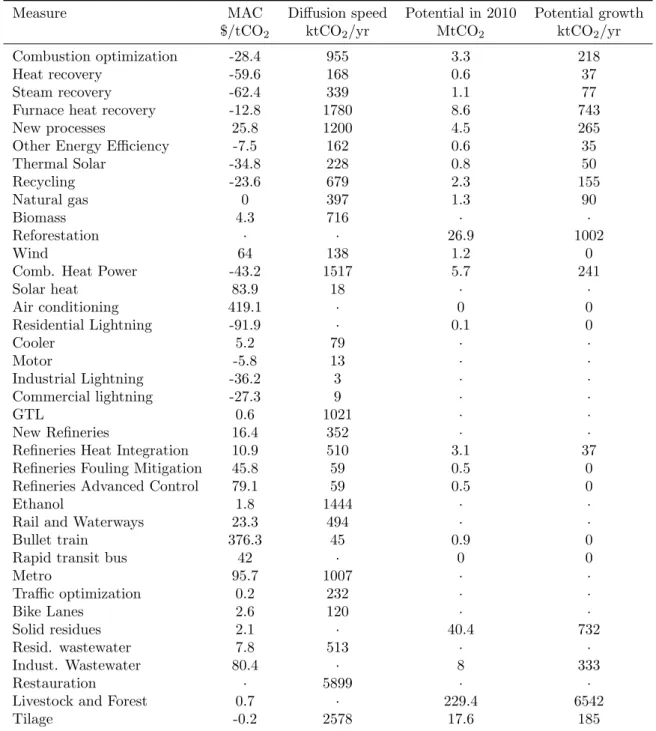
While the list of measures and their cost can be used di-rectly in our spreadsheet program (see the first two columns of Tab.1), our program requires the full-abatement po-tential and diffusion speed. Since the diffusion speed and the full-abatement potential were not reported separately, we have to reconstruct them with indirect methods, us-ing the emission-reduction pathways that were provided to MACTool. For each measure, the shape of the emission-reduction pathways can be classified in one out of three cases.

In the first case, emission-reduction pathways may be approximated by a two-phases piecewise-linear function as

Figure 3: Emission reductions achieved over time thanks to recycling. This particular emission-reduction measure illus-trates that many emission reduction pathways (the plus signs +) may be approximated by a piecewise-linear curve (in red). The slope of the first piece provides the diffusion speed for that measure. The second part is interpreted as the maximum po-tential, that grows over time.

in Fig.3. In this case, the diffusion speed is given by the slope of the first piece, and the second phase is interpreted as the growing full potential. About half the measures fall in this category.

Other emission-reduction pathways may be approxi-mated by a single linear diffusion (Fig.4a). In this case, the full potential is not binding before 2030. We calibrate the diffusion speed from the slope of the penetration path-way, and denote the lack of data on the full potential with a dot (·) in the two last columns of Tab.1.

In some other cases the emission-reduction pathway lacks the first phase; abatement immediately “jumps” to a growing full-potential (Fig.4b). We denote them with a dot in the diffusion speed column in Tab.1. There is usually a handful of such cases in MAC curves exercises. One example from the Brazilian study is solid residues management. In the emission-reduction pathway, solid residues management is able to reduce emissions by more than 40 MtCO2 in one year, and then grow at less than

1 MtCO2/yr. From the perspective of the user of a MAC

curve, it is unclear whether this should be considered as a shortcoming in the data (if the investigation could not identify the constraints that limit the diffusion of solid residues management), or a realistic emission-reduction pathway (if solid residues management can actually save lots of GHG in a short time lapse).7 _{To avoid this situation}

7 _{Livestock and forest management is a particular example.}

In the emission-reduction pathways, this measures allows to save 229 MtCO2, that is almost one third of the total abatement potential

by 2030, as soon as 2010. Since Brazil has already managed to reduce drastically its emissions from deforestation (-80% between 2004 and 2009), the study considered that this mitigation option is already enforced. Sustaining such effort over a long period will require that productivity gains in the livestock sector free-up pasture land fast enough to accommodate the growth of the livestock-agriculture sec-tor without deforesting, as recommended in the Brazil Low-carbon study (de Gouvello,2010).

Measure MAC Diffusion speed Potential in 2010 Potential growth $/tCO2 ktCO2/yr MtCO2 ktCO2/yr

Combustion optimization -28.4 955 3.3 218

Heat recovery -59.6 168 0.6 37

Steam recovery -62.4 339 1.1 77

Furnace heat recovery -12.8 1780 8.6 743

New processes 25.8 1200 4.5 265

Other Energy Efficiency -7.5 162 0.6 35

Thermal Solar -34.8 228 0.8 50 Recycling -23.6 679 2.3 155 Natural gas 0 397 1.3 90 Biomass 4.3 716 · · Reforestation · · 26.9 1002 Wind 64 138 1.2 0

Comb. Heat Power -43.2 1517 5.7 241

Solar heat 83.9 18 · · Air conditioning 419.1 · 0 0 Residential Lightning -91.9 · 0.1 0 Cooler 5.2 79 · · Motor -5.8 13 · · Industrial Lightning -36.2 3 · · Commercial lightning -27.3 9 · · GTL 0.6 1021 · · New Refineries 16.4 352 · ·

Refineries Heat Integration 10.9 510 3.1 37

Refineries Fouling Mitigation 45.8 59 0.5 0

Refineries Advanced Control 79.1 59 0.5 0

Ethanol 1.8 1444 · ·

Rail and Waterways 23.3 494 · ·

Bullet train 376.3 45 0.9 0

Rapid transit bus 42 · 0 0

Metro 95.7 1007 · · Traffic optimization 0.2 232 · · Bike Lanes 2.6 120 · · Solid residues 2.1 · 40.4 732 Resid. wastewater 7.8 513 · · Indust. Wastewater 80.4 · 8 333 Restauration · 5899 · ·

Livestock and Forest 0.7 · 229.4 6542

Tilage -0.2 2578 17.6 185

(a) No potential (b) No speed

Figure 4: Emission reductions achieved over time thanks to traffic optimization and management of solid residues. For some abatement measures, the data needed to calibrate our model cannot be derived from the emission-reduction pathways. Traffic optimization (a)is an example of measure for which the long term potential is not binding because it cannot be reached before 2030. Solid residues (b) exemplifies that for some other measures, the diffusion speed cannot be assessed — either it was not investigated, or the measure can reach its full potential in less than one year.

in the future, we recommend that the terms of reference for the experts in charge of collecting data on emission reductions options should explicitly ask to report possible diffusion speeds (Appendix B).

Finally, some emission-reduction measures (reforesta-tion, air conditioning and rapid bus transit) were included in the list while lacking either a marginal abatement cost or an emission scenario. These measures, as well as those for which the diffusion speed could not be estimated, are dis-carded for the rest of the analysis. The remaining options allow to reduce Brazilian emissions in 2030 by 223 MtCO2

(compared with 812 MtCO2 in the original MAC curve).

2.2. Results

In a first simulation, we run our spreadsheet model to design the socially optimal strategy to achieve 223 MtCO2

of emission reductions by 2030. The optimal emission-reduction strategy has the following characteristics (for transparency and reproducibility purposes, detailed results are displayed inAppendix C).

First, all negative-cost measures are introduced at full speed from year 2010, independently of the emission-reduction target. Indeed, these measures are desirable per se, as they bring more benefits than costs even in the absence of any carbon pricing or climate change impacts.8

Second, the least-cost strategy is to implement the positive-cost measures as late as possible, to benefit from the discount rate. This means that under climate targets expressed as an emission reduction in one point in time, such as -30% by 2030, the two-phase penetration pictured

8 _{Remember that our framework accounts for implementation}

barriers that lower the speed at which emission reduction options may be implemented, but do not increase their cost.

in Fig.3is not optimal for positive-cost measures. A bet-ter solution is to delay the implementation such that the maximum potential is reached just in time, when the tar-get needs to be achieved.9

Finally, the optimal emission reduction pathway to achieve 223 MtCO2in 2030 leads to 127 MtCO2of emission

reduc-tions in 2020.

To investigate how focusing on short-term targets may lead to suboptimal outcomes, we run a second simula-tion with the only constraint of reducing emissions by 127 MtCO2 in 2020. We then investigate how the

“opti-mal” solution provided by our model in this case compares to the first simulation.

In line with Vogt-Schilb and Hallegatte (2014), the least-cost strategy for 2010-2020 uses different emission-reduction options, depending on whether the strategy aims at a short-term target (127 MtCO2in 2020) or at a

longer-term one (223 MtCO2 in 2030). This is shown in Fig.5,

which depicts emission reductions achieved by 2020 in the two strategies, for selected emission reduction options. We chose the five emission-reduction measures with the high-est difference between the two scenarios. The simulation that ends in 2020 uses notably less investment in metro and other clean transportation infrastructure, and more heat integration and other marginal improvements in existing refineries than what the 2030 simulation does by 2020.

Indeed, clean transportation infrastructure is charac-terized by a large abatement potential, and high cost per ton of CO2 avoided. As illustrated in Fig.6, these

op-tions are not implemented when short-term target masks

9_{This is a downside of targets expressed in terms of reductions at}

one point in time. If the climate mitigation target was expressed in terms of a carbon budget (consistently with climate change physics,

Zickfeld et al.,2009), then the two-phase penetration target would be optimal (Vogt-Schilb and Hallegatte,2014, section 4).

0 2 4 6 8 10 12

Metro Rail and Waterways

Bullet train Refineries Heat Integration New processes M tC O2 Emission reductions in 2020

In the 2030 strategy In the 2020 strategy

Figure 5: Comparison of emission reduction achieved in 2020 with a set of measures when the 2020 target is the final target vs. when it is a milestone toward a more ambitious 2030 target. The picture shows the five emission-reduction for which the difference between the two strategies are the largest.

M a rg in a l co st $/t C O2 3 1 2 4 5 Potential MtCO2/yr in2020 D₂₀₂₀ (a) Achievable by 2020 M a rg in a l co st $/t C O2 1 2 3 4 5 Potential MtCO2/yr in2030 D₂₀₃₀ (b) Achievable by 2030

Figure 6: Two achievable-potential MAC curves, built for 2020 and 2030. The 2020 MAC curve (a)suggests that the 2020 target (D2020) can be met using only options 1–4, disregarding option 5 before 2020. But then only a fraction of option 5 could

be implemented between 2020 and 2030. The 2030 MAC curve (b) however shows that options 1–5 should be implemented by 2030 to meet the D2030target. For option 5 to deliver all the abatement listed by 2030, it should be implemented before 2020.

the longer-term target. In addition, clean transportation infrastructure also takes a long time to implement, mean-ing that in the 2030 scenario, it is implemented as fast as possible — confirming the need for short term investment in clean infrastructure, as recently advocated byWaisman et al. (2012); Framstad and Strand (2013); Kopp et al.

(2013);Lecocq and Shalizi(2014) andAvner et al.(2014). Moreover, because it takes so long to build clean trans-portation infrastructure, not starting doing it before 2020 closes the door to deeper emission reductions by 2030. In-deed, reaching the 2030 target requires the implementa-tion of 95 addiimplementa-tional MtCO2 of abatement between 2020

and 2030. However, a 2020-2030 strategy would be able to save 84 MtCO2additionally at best, since not enough time

would be left to deploy time intensive solutions. This new low-carbon scenario would therefore be short 11 MtCO2or

12% in 2030 compared to the first best. In other words, the 2030 target becomes impossible to achieve after 2020, as the limited diffusion speed prevents high-abatement-potential options to achieve their optimal 2030 level in only 10 years. This is an example of how delayed action in key sectors can create carbon lock-ins.

3. Conclusion

In order to put the economy on the track to deep de-carbonization, 9 MtCO2of abatement achieved with metro

may be worth more than 11 MtCO2achieved with

energy-efficiency improvements in refineries; for metro avoids lock-ing the transportation system in carbon-intensive patterns, while energy-efficiency improvement in refineries has lim-ited long-term potential.

Regardless of the process used to generate them, MAC curves cannot communicate this type of information to decision makers: they appear as static abatement supply curves, leaving any caveat regarding the dynamic aspect of mitigation strategies to method sections or footnotes. An easy solution to mitigate this issue may be to systemati-cally display flipped MAC curves next to the correspond-ing emission-reduction pathway, also known as a wedge curve (Fig.2).

More generally, the abatement potential and cost are not sufficient information to schedule emission-reduction measures. Both a long-term objective and the speed at which each option may deliver abatement are instrumen-tal in deciding on the quantity and quality of short-term emission reductions.

With this information, decision makers can design poli-cies aiming to achieve two objectives. The first is to re-move implementation barriers on negative- and low-cost options. The second is to ensure short-term targets are met with abatement of sufficient quality – that is with-out under-investing in the ambitious abatement measures required to achieve long-term targets.

Acknowledgments

We thank Pierre Audinet, Mook Bangalore, Luis Gon-zalez, Jean-Charles Hourcade, Pedzi Makumbe, Baptiste Perissin-Fabert, Julie Rozenberg, Supachol Suphachalasai, three anonymous referees and seminar participants at the French Minist`ere du D´eveloppement Durable, the World Bank, and the International Energy Agency for useful dis-cussions on the work performed here. All remaining er-rors are the authors’ responsibility. We thank the ESMAP (World Bank) for financial support. The views expressed in this paper are the sole responsibility of the authors. They do not necessarily reflect the views of the World Bank, its executive directors, or the countries they rep-resent. A previous version of this paper is Vogt-Schilb et al.(2014)

References

Acemoglu, D., Aghion, P., Bursztyn, L., Hemous, D., 2012. The environment and directed technical change. American Economic Review 102 (1), 131–166.

Allcott, H., Greenstone, M., 2012. Is there an energy efficiency gap? Journal of Economic Perspectives 26 (1), 3–28.

Avner, P., Rentschler, J. E., Hallegatte, S., 2014. Carbon price effi-ciency: Lock-in and path dependence in urban forms and trans-port infrastructure. World Bank Policy Research Working Paper 6941.

Azar, C., Sand´en, B. A., 2011. The elusive quest for technology-neutral policies. Environmental Innovation and Societal Transi-tions 1 (1), 135–139.

Bertram, C., Johnson, N., Luderer, G., Riahi, K., Isaac, M., Eom, J., 2014. Carbon lock-in through capital stock inertia associated with weak near-term climate policies. Technological Forecasting and Social Change (forthcoming).

Brunner, S., Flachsland, C., Marschinski, R., 2012. Credible com-mitment in carbon policy. Climate Policy 12 (2), 255–271. CE Delft, 2012. Marginal abatement cost curves for heavy duty

ve-hicles. Background report, Arno Schroten, Geert Warringa and Mart Bles, Delft.

Climate Works Australia, 2010. Low carbon growth plan for Aus-tralia. ClimateWorks Australia Clayton.

Collins, M., Knutti, R., Arblaster, J. M., Dufresne, J.-L., Fichefet, T., Friedlingstein, P., Gao, X., Gutowski, W. J., Johns, T., Krin-ner, G., 2013. Long-term climate change: projections, commit-ments and irreversibility. In: Climate Change 2013: The Physi-cal Science Basis. Contribution of Working Group I to the Fifth Assessment Report of the Intergovernmental Panel on Climate Change.

Davis, S. J., Cao, L., Caldeira, K., Hoffert, M. I., 2013. Rethinking wedges. Environmental Research Letters 8 (1), 011001.

de Gouvello, C., 2010. Brazil Low-carbon Country Case Study. The World Bank, Washington DC, USA.

DECC, 2011. Impact assessment of fourth carbon budget level. Im-pact Assessment DECC0054, Department of Energy and Climate Change, UK.

del Rio Gonzalez, P., 2008. Policy implications of potential conflicts between short-term and long-term efficiency in CO2 emissions abatement. Ecological Economics 65 (2), 292–303.

Enkvist, P., Naucl´er, T., Rosander, J., 2007. A cost curve for green-house gas reduction. McKinsey Quarterly 1, 34.

ESMAP, 2012. Planning for a low carbon future: Lessons learned from seven country studies. Knowledge series 011/12, Energy Sec-tor Management Assistance Program - The World Bank, Wash-ington DC, USA.

ESMAP, 2014. Modeling tools and e-learning: MACTool. URLhttp://esmap.org/MACTool

Fischer, C., Preonas, L., 2010. Combining policies for renewable en-ergy: Is the whole less than the sum of its parts? International Review of Environmental and Resource Economics 4, 51–92. Framstad, N. C., Strand, J., 2013. Energy intensive infrastructure

in-vestments with retrofits in continuous time: Effects of uncertainty on energy use and carbon emissions. World bank policy research working paper, 6430.

Gerlagh, R., Kverndokk, S., Rosendahl, K., 2009. Optimal timing of climate change policy: Interaction between carbon taxes and innovation externalities. Environmental and Resource Economics 43 (3), 369–390.

Giraudet, L.-G., Houde, S., 2013. Double moral hazard and the en-ergy efficiency gap.

Golombek, R., Greaker, M., Hoel, M., 2010. Carbon taxes and inno-vation without commitment. The B.E. Journal of Economic Anal-ysis & Policy 10 (1).

Gr¨ubler, A., Messner, S., 1998. Technological change and the timing of mitigation measures. Energy Economics 20 (5-6), 495–512. Gr¨ubler, A., Naki´cenovi´c, N., Victor, D. G., 1999. Dynamics of

en-ergy technologies and global change. Enen-ergy policy 27 (5), 247– 280.

Grubb, M., Chapuis, T., Ha-Duong, M., 1995. The economics of changing course: Implications of adaptability and inertia for op-timal climate policy. Energy Policy 23 (4-5), pp. 417–431. Ha-Duong, M., Grubb, M., Hourcade, J., 1997. Influence of

socioe-conomic inertia and uncertainty on optimal CO2-emission abate-ment. Nature 390 (6657), 270–273.

Haab, T., 2007. Environmental economics: Look! it’s a carbon sup-ply curve.

URLhttp://env-econ.net/2007/07/look-its-a-real.html

Hallegatte, S., Fay, M., Vogt-Schilb, A., 2013. Green industrial poli-cies: When and how. World Bank Policy Research Working Pa-per (6677).

Iyer, G., Hultman, N., Eom, J., McJeon, H., Patel, P., Clarke, L., 2014. Diffusion of low-carbon technologies and the feasibility of long-term climate targets. Technological Forecasting and Social Change (forthcoming).

Jenkins, J. D., 2014. Political economy constraints on carbon pric-ing policies: What are the implications for economic efficiency, environmental efficacy, and climate policy design? Energy Policy. Kalkuhl, M., Edenhofer, O., Lessmann, K., 2012. Learning or lock-in: Optimal technology policies to support mitigation. Resource and Energy Economics 34, 1–23.

Kesicki, F., 2012a. Intertemporal issues and marginal abatement costs in the UK transport sector. Transportation Research Part D: Transport and Environment 17 (5), 418–426.

Kesicki, F., 2012b. Marginal abatement cost curves: Combining en-ergy system modelling and decomposition analysis. Environmental Modeling & Assessment.

Kesicki, F., Ekins, P., 2012. Marginal abatement cost curves: a call for caution. Climate Policy 12 (2), 219–236.

Kolstad, C., Urama, K., Broome, J., Bruvoll, A., Olvera, M. C., Fullerton, D., Gollier, C., Hanemann, W., Hassan, R., Jotzo, F., Khan, M., Meyer, L., Mundaca, L., 2014. Social, economic and ethical concepts and methods. In: Climate Change 2014: Miti-gation of Climate Change. Contribution of Working Group III to the Fifth Assessment Report of the Intergovernmental Panel on Climate Change.

Kopp, A., Block, R. I., Iimi, A., 2013. Turning the Right Corner: Ensuring Development through a Low-Carbon Transport Sector. The World Bank.

Lecocq, F., Shalizi, Z., 2014. The economics of targeted mitigation in infrastructure. Climate Policy 14 (2), 187–208.

Lecuyer, O., Quirion, P., 2013. Can uncertainty justify overlapping policy instruments to mitigate emissions? Ecological Economics 93, 177–191.

Lecuyer, O., Vogt-Schilb, A., 2014. Optimal transition from coal to gas and renewable power under capacity constraints and adjust-ment costs. World Bank Policy Research Working Paper 6985. Luderer, G., Bertram, C., Calvin, K., Cian, E. D., Kriegler, E.,

2013. Implications of weak near-term climate policies on long-term

mitigation pathways. Climatic Change, 1–14.

McKinsey, 2007. Reducing US greenhouse gas emissions: How much at what cost? Tech. rep., McKinsey & Company.

McKinsey, 2009. Pathways to a low-carbon economy: Version 2 of the global greenhouse gas abatement cost curve. Tech. rep., McKinsey & Company.

NERA, 2011a. The demand for greenhouse gas emissions reduction investments: An investors’ marginal abatement cost curve for kazakhstan. Prepared for the european bank for reconstruction and development, NERA Economic Consulting and Bloomberg New Energy Finance.

NERA, 2011b. The demand for greenhouse gas emissions reductions: An investors’ marginal abatement cost curve for turkey. Prepared for the european bank for reconstruction and development, NERA Economic Consulting and Bloomberg New Energy Finance. NERA, 2012. The demand for greenhouse gas emissions reduction

investments: An investors’ marginal abatement cost curve for ukraine. Prepared for the european bank for reconstruction and development, NERA Economic Consulting and Bloomberg New Energy Finance.

O’Brien, D., Shalloo, L., Crosson, P., Donnellan, T., Farrelly, N., Finnan, J., Hanrahan, K., Lalor, S., Lanigan, G., Thorne, F., Schulte, R., 2014. An evaluation of the effect of greenhouse gas accounting methods on a marginal abatement cost curve for irish agricultural greenhouse gas emissions. Environmental Science & Policy 39, 107–118.

Pacala, S., Socolow, R., 2004. Stabilization wedges: Solving the cli-mate problem for the next 50 years with current technologies. Science 305 (5686), 968–972.

Parry, I. W. H., Evans, D., Oates, W. E., 2014. Are energy effi-ciency standards justified? Journal of Environmental Economics and Management 67 (2), 104–125.

Pellerin, S., Bami`ere, L., Angers, D., B´eline, F., Benoˆıt, M., Bu-tault, J., Chenu, C., Colnenne-David, C., De Care, S., Delame, N., Doreau, M., Dupraz, P., Faverdin, P., Garcia-Launay, F., Has-souna, M., H´enault, C., Jeuffroy, M., Klumpp, K., Metay, A., Moran, D., Recous, S., Samson, E., Savini, I., Pardon, L., 2013. Quelle contribution de l’agriculture fran¸caise `a la r´eduction des ´emissions de gaz `a effet de serre? Potentiel d’att´enuation et coˆut de dix actions techniques. Synth`ese du rapport d’´etude, INRA, France.

Riahi, K., Kriegler, E., Johnson, N., Bertram, C., den Elzen, M., Eom, J., Schaeffer, M., Edmonds, J., Isaac, M., Krey, V., Long-den, T., Luderer, G., M´ejean, A., McCollum, D. L., Mima, S., Turton, H., van Vuuren, D. P., Wada, K., Bosetti, V., Capros, P., Criqui, P., Hamdi-Cherif, M., Kainuma, M., Edenhofer, O., 2014. Locked into copenhagen pledges — implications of short-term emission targets for the cost and feasibility of long-short-term cli-mate goals. Technological Forecasting and Social Change (forth-coming).

Rosendahl, K. E., 2004. Cost-effective environmental policy: impli-cations of induced technological change. Journal of Environmental Economics and Management 48 (3), 1099–1121.

Rozenberg, J., Vogt-Schilb, A., Hallegatte, S., 2014. Transition to clean capital, irreversible investment and stranded assets. World Bank Policy Research Working Paper (6859).

Rubin, E. S., Cooper, R. N., Frosch, R. A., Lee, T. H., Marland, G., Rosenfeld, A. H., Stine, D. D., 1992. Realistic mitigation options for global warming. Science 257 (5067), 148–149.

Sachs, J., Tubiana, L., Guerin, E., Waisman, H., Mas, C., Colombier, M., Schmidt-Traub, G., 2014. Pathways to deep decarbonization. Interim 2014 report, Deep Decarbonization Pathways Project. Sand´en, B. A., Azar, C., 2005. Near-term technology policies for

long-term climate targets—economy wide versus technology spe-cific approaches. Energy Policy 33 (12), 1557–1576.

Steinacher, M., Joos, F., Stocker, T. F., 2013. Allowable carbon emissions lowered by multiple climate targets. Nature 499 (7457), 197–201.

Tsvetanov, T., Segerson, K., 2013. Re-evaluating the role of energy efficiency standards: A behavioral economics approach. Journal of Environmental Economics and Management 66 (2), 347–363.

Vogt-Schilb, A., Hallegatte, S., 2014. Marginal abatement cost curves and the optimal timing of mitigation measures. Energy Policy 66, 645–653.

Vogt-Schilb, A., Hallegatte, S., de Gouvello, C., 2014. Long-term mitigation strategies and marginal abatement cost curves: a case study on Brazil. World Bank Policy Research (6808).

Vogt-Schilb, A., Meunier, G., Hallegatte, S., 2012. How inertia and limited potentials affect the timing of sectoral abatements in op-timal climate policy. World Bank Policy Research Working Paper 6154.

Waisman, H., Guivarch, C., Grazi, F., Hourcade, J. C., 2012. The Imaclim-R model: infrastructures, technical inertia and the costs of low carbon futures under imperfect foresight. Climatic Change 114 (1), 101–120.

W¨achter, P., 2013. The usefulness of marginal CO2-e abatement cost curves in Austria. Energy Policy 61, 1116–1126.

Williams, J. H., DeBenedictis, A., Ghanadan, R., Mahone, A., Moore, J., Morrow, W. R., Price, S., Torn, M. S., 2012. The technology path to deep greenhouse gas emissions cuts by 2050: The pivotal role of electricity. Science 335 (6064), 53–59. Wilson, C., Grubler, A., Bauer, N., Krey, V., Riahi, K., 2013. Future

capacity growth of energy technologies: are scenarios consistent with historical evidence? Climatic Change 118 (2), 381–395. World Bank, 2012. Inclusive green growth : the pathway to

sustain-able development. World Bank, Washington, D.C.

World Bank, 2013. Applying abatement cost curve methodology for low-carbon strategy in Changning district, Shanghai. Tech. Rep. 84068, The World Bank.

Zickfeld, K., Eby, M., Matthews, H. D., Weaver, A. J., 2009. Set-ting cumulative emissions targets to reduce the risk of dangerous climate change. Proceedings of the National Academy of Sciences 106 (38), 16129–16134.

Appendix A. Model

We extend the model proposed byVogt-Schilb and Hal-legatte (2014). As inputs, the model takes a set of mea-sures (indexed by i), their respective abatement potential Ai,t, (marginal) abatement costs ci,10 maximum diffusion

speeds vi, an abatement target a?T, set for a date in the

future T (e.g. 2020 or 2030), and a discount rate r. The model computes the least-cost schedule ai,tof

emis-sion reductions done with each measure i at each time t: min

ai,t

X

i,t

e−rtciai,t (A.1)

The model takes into account the constraint set by maxi-mum abatement potentials:11

∀(i, t), ai,t ≤ Ai,t (A.2)

The second constraint on emission reduction is that they cannot grow faster than the diffusion speed vi, such that:

ai,t+1≤ ai,t+ vi (A.3)

10_{The model assumes that abatement costs are linear, such that}

marginal and average cost coincide.

11 _{In the model proposed byVogt-Schilb and Hallegatte(2014),}

abatement potentials do not evolve over time. This is the only ex-tension we propose.

Finally, the abatement target sets the following constraint: X

i

ai,T ≥ a?T (A.4)

An Excel implementation of this model is available on-line.

Appendix B. Information collection guidance The following proposes guidance on how data on emis-sion reduction measures could be collected to take into account the findings of this paper. The objective is to collect data that can be used to build emission reduction pathways and MAC curves in order to inform climate mit-igation policies. Asking specifically to disclosure assump-tions on the diffusion speed of each option (3c) should help identify bottlenecks preventing some measures to be im-plemented.

Note that collecting this data does not require more work that what is currently done to build MAC curves from expert surveys; clarifying the difference between im-plementation speed and full technical potential may actu-ally facilitate the data-gathering process.

Of course, this sketch should be adapted to local condi-tions; for instance, it should account for existing plans and projections when defining emission baseline and abatement potentials.

1. Inventory of existing GHG emissions

(a) Provide the list of GHG emissions at a given date in the recent past. Chose the most recent date for which data is available .

(b) Provide a breakdown of these emissions by sec-tor, e.g. power generation, industry, buildings, transportation, agriculture. Use sub-sectors where possible, for instance as provided by the Inter-national Standard Industrial Classification. (c) Describe current output of these sectors.

i. Use physical measures of output when pos-sible, e.g:

A. In the transportation sector, use passenger-kilometer and ton-passenger-kilometer.

B. In the power sector, use MWh/yr. C. In the residential sector, use number of

inhabitants at given comfort.

ii. Express these emissions in CO2equivalent

using accepted conversion factors.

2. Prospective: provide projections of future GHG emis-sions reported in1 using the same breakdown. Re-port relevant drivers, such as population projections, GDP growth, etc.

3. List available emission-reduction measures (a) Full technological potentials

i. Provide emission intensity of each activity (e.g., gCO2/km).

ii. Provide maximum potential with today’s technology: e.g. hydro power limited by river availability, electric vehicles limited by range. If relevant provide maximum penetration rate given political and societal constraints (e.g. if nuclear power is unac-ceptable).

(b) Costs

i. Report Capex and Opex separately

A. Report input-efficiency (e.g. fuel-efficiency and fuel type)

B. Report input prices (report taxes sepa-ratedly)

ii. Report domestic and foreign expenses sep-arately.

iii. Report costs used to pay domestic salaries separately

For instance, a photovoltaic power module can be imported but the installation is paid to a local worker; avoided gasoline use from electric vehicles means less oil imports, but also less tax revenue.

(c) Speed at which new technologies may enter the market. This piece of data assesses the speed at which each option can be implemented – tak-ing into account the required accumulation of human and physical capital.

i. Report typical capital lifetimes for consid-ered technologies and related technologies in the sector — e.g. cars typically live 12 years.

ii. Report past penetration rates for similar technologies in the sector — e.g. diesel sales took 30 years to go from 0 to 50% in the past.

iii. Report current bottlenecks (institutional bar-riers, available resources) — e.g. available workforce can retrofit 100 000 dwellings per year.

2010 2011 2012 2013 2014 2015 2016 2017 2018 2019 2020 Com bustion opti m ization 0.96 1 .91 2.87 3.82 4.19 4.41 4.63 4.84 5.06 5.28 5.50 Heat reco v ery 0.17 0.34 0.51 0.67 0.78 0.82 0.86 0.90 0.93 0.97 1.01 Steam reco v ery 0.34 0.68 1.02 1.36 1.49 1.56 1.64 1.72 1.80 1.87 1.95 F urnace heat reco v ery 1.78 3.56 5.34 7.12 8.90 10.69 12.47 13.84 14.58 15.32 16.07 New pro cesses -Other Energy Efficiency 0.16 0.33 0.49 0. 6 5 0. 75 0. 79 0. 83 0. 86 0 .90 0.93 0.97 Thermal Solar 0.23 0.46 0.68 0.91 1.06 1.11 1.16 1.21 1.26 1.31 1.36 Recycling 0.68 1.36 2.04 2.72 2.98 3.13 3.29 3.44 3.60 3.76 3.91 Natural gas 0.40 0.79 1.19 1.59 1.74 1.83 1.92 2.01 2.10 2.20 2.29 Biomass 0.72 1.43 2.15 2.87 3.58 4.30 5.02 5.73 6.45 7.17 7.89 Wind -Com b. Heat P o w er 1.52 3.04 4.55 6.07 6.68 6.92 7.16 7.40 7.64 7.88 8.13 Solar heat 0.02 0.04 0.06 0.07 0.09 0.11 0.13 0.15 0.17 0.18 0.20 Co oler 0.08 0.16 0.24 0.32 0.40 0.48 0.56 0.64 0.71 0.79 0.87 Motor 0.01 0.03 0.04 0.05 0.07 0.08 0.09 0.11 0.12 0.13 0.15 Industrial Ligh tning 0.00 0.01 0.01 0.02 0. 0 2 0. 02 0. 03 0. 03 0. 03 0 .04 0.04 Commercial ligh tning 0.01 0.02 0.03 0.04 0.05 0.06 0.07 0.07 0.08 0.09 0.10 GTL 1.02 2.04 3.06 4.09 5.11 6.13 7.15 8.17 9.19 10.21 11.24 New Refineries 0.35 0.70 1.06 1.41 1.76 2.11 2.47 2.82 3.17 3.52 3.87 Refineries Heat In tegration -Refineries F ouling Mitigation -Refineries Adv anced Con trol -Ethanol 1.44 2.89 4.33 5.78 7.22 8.67 10.11 11.56 13.00 14.44 15.89 Rail and W aterw a ys 0.49 0.99 1.48 1.98 2.47 2.97 3.46 3.96 4.45 4.95 5.44 Bullet train 0.01 0.06 0.10 0. 15 0. 19 0 .24 0.28 0.33 0.38 0.42 0.47 Metro 1.01 2.02 3.02 4.03 5.04 6.05 7.05 8.06 9.07 10.08 11.09 T raffic optimization 0.23 0.47 0 .70 0.93 1.16 1.40 1.63 1.86 2.10 2.33 2.56 Bik e Lanes 0.12 0.24 0.36 0.48 0.60 0.72 0.84 0.97 1.09 1.21 1.33 Resid. w astew ater 0.51 1.03 1.54 2.05 2.57 3.08 3.59 4.11 4.62 5.13 5.65 Tilage 2.58 5.16 7.74 10.31 12.89 15.47 18.05 18.91 19.09 19.28 19.46

2010 2011 2012 2013 2014 2015 2016 2017 2018 2019 2020 Com bustion opti m ization 0.96 1 .91 2.87 3.82 4.19 4.41 4.63 4.84 5.06 5.28 5.50 Heat reco v ery 0.17 0.34 0.51 0.67 0.78 0.82 0.86 0.90 0.93 0.97 1.01 Steam reco v ery 0.34 0.68 1.02 1.36 1.49 1.56 1.64 1.72 1.80 1.87 1.95 F urnace heat reco v ery 1.78 3.56 5.34 7.12 8.90 10.69 12.47 13.84 14.58 15.32 16.07 New pro cesses -1.16 2.36 3.56 4.77 5.97 7.17 Other Energy Efficiency 0.16 0.33 0.49 0.65 0. 7 5 0. 79 0. 83 0. 86 0. 90 0 .93 0.97 Thermal Solar 0.23 0.46 0.68 0.91 1.06 1.11 1.16 1.21 1.26 1.31 1.36 Recycling 0.68 1.36 2.04 2.72 2.98 3.13 3.29 3.44 3.60 3.76 3.91 Natural gas 0.40 0.79 1.19 1.59 1.74 1.83 1.92 2.01 2.10 2.20 2.29 Biomass 0.72 1.43 2.15 2.87 3.58 4.30 5.02 5.73 6.45 7.17 7.89 Wind -0.14 0.28 0.41 Com b. Heat P o w er 1.52 3.04 4.55 6.07 6.68 6.92 7.16 7.40 7.64 7.88 8.13 Solar heat -0.02 0.04 Co oler 0.08 0.16 0.24 0.32 0.40 0.48 0.56 0.64 0.71 0.79 0.87 Motor 0.01 0.03 0.04 0.05 0.07 0.08 0.09 0.11 0.12 0.13 0.15 Industrial Ligh tning 0.00 0.01 0.01 0.02 0.02 0. 0 2 0. 03 0. 03 0. 03 0. 04 0.04 Commercial ligh tning 0.01 0.02 0.03 0.04 0.05 0.06 0.07 0.07 0.08 0.09 0.10 GTL 1.02 2.04 3.06 4.09 5.11 6.13 7.15 8.17 9.19 10.21 11.24 New Refineries -0.35 0.70 1.06 1.41 1.76 2.11 2.47 2.82 3.17 3.52 Refineries Heat In tegration -0.51 1.02 1.53 2.04 2.55 3.06 3.57 Refineries F ouling Mitigation -0.06 0.12 0.18 0.24 Refineries Adv anced Con trol -0.03 0.09 0.15 Ethanol 1.44 2.89 4.33 5.78 7.22 8.67 10.11 11.56 13.00 14.44 15.89 Rail and W aterw a ys -0.49 0.99 1.48 1.98 2.47 2.97 3.46 3.96 Bullet train -Metro -1.01 2.02 T raffic optimization 0.23 0.47 0. 70 0.93 1.16 1.40 1.63 1.86 2.10 2.33 2.56 Bik e Lanes 0.12 0.24 0. 36 0.48 0.60 0.72 0.84 0.97 1.09 1.21 1.33 Resid. w astew ater 0.51 1.03 1.54 2.05 2.57 3.08 3.59 4.11 4.62 5.13 5.65 Tilage 2.58 5.16 7.74 10.31 12.89 15.47 18.05 18.91 19.09 19.28 19.46