Airborne protected military satellite communications : analysis of open-loop pointing and closed-loop tracking with noisy platform attitude information

ACHNVES

MASSACHUSETTS INSfMUT

Airborne Protected

Military Satellite Communications: j3 j13

Analysis of

LIBRARIES

Open-Loop Pointing and Closed-Loop Tracking

with Noisy Platform Attitude Information

by

William D. Deike

B.S. Electrical Engineering

United States Air Force Academy, 2008

Submitted to the Department of Aeronautics and Astronautics

in partial fulfillment of the requirements for the degree of

Master of Science

at the

MASSACHUSETTS INSTITUTE OF TECHNOLOGY

May 2010

'I0

n(4L

@

Massachusetts Institute of Technology 2010. All rights reserved.

Author ...

-Departnent of Aeronautics and Astronautics

May 21, 2010

C er ifed by ... ... ... .... .

Certified by:..,

₆₂

Timothy Gallagher, Ph.D.

Technical Staff, MIT Lincoln Laboratory

Thesis Supervisor

Certified by: ..

...

Steven R. Hall, Ph.D.

Professor of Aeronautics and Astronautics

/. Tkesis Supervisor

A ccepted by ...

. ...

Eytan H. Modiano, Ph.D.

Associate Professor of Aeronautics and Astronautics

Chair, Committee on Graduate Students

Airborne Protected Military Satellite Communications:

Analysis of Open-Loop Pointing and Closed-Loop Tracking

with Noisy Platform Attitude Information

by

William D. Deike

Submitted to the Department of Aeronautics and Astronautics on May 21, 2010, in partial fulfillment of the

requirements for the degree of Master of Science

Abstract

U.S. military assets' increasing need for secure global communications has led to the design and

fabri-cation of airborne satellite communifabri-cation terminals that operate under protected security protocol. Protected transmission limits the closed-loop tracking options to eliminate pointing error in the open-loop pointing solution. In an airborne environment, aircraft disturbances and noisy attitude information affect the open-loop pointing performance. This thesis analyzes the open-loop pointing and closed-loop tracking performance in the presence of open-loop pointing error and uncertainty in the received signal to assess hardware options relative to performance requirements. Results from the open-loop analysis demonstrate unexplained harmonics at integer frequencies while the aircraft is banked, azimuth and elevation errors independent of the inertial pointing vector and aircraft's yaw angle, and uncorrelated azimuth and elevation errors for aircraft pitch and roll angles of +100 and ±30', respectively. Several conclusions are drawn from the closed-loop tracking analysis. The distribution of the average noise power has a stronger influence than the distribution of the received isotropic power on the signal-to-noise ratio distribution. The defined step-tracking algorithm reduces pointing error in the open-loop pointing solution for a pedestal experiencing aircraft disturbances and random errors from the GPS/INS. The rate of performance improvement as a function of the number of hops is independent of the antenna aperture size and the GPS/INS unit. Pointing per-formance relative to the HPBW is independent of the antenna aperture size and GPS/INS unit for on-boresight, but not for off-boresight. With signal-to-noise ratios averaged over 100 hops and pointing biases less than or equal to 0.5 the half-power beamwidth, the step-tracking algorithm reduces the pointing error to within 0.1 the half-power beamwidth of the boresight, for all tested configurations. The overall system performance is bounded by the open-loop pointing solution, which is based on hardware selection. Closed-loop tracking performance is a function of the number of sampled hops and is for the most part independent of the hardware selection.

Thesis Supervisor: Timothy Gallagher, Ph.D. Title: Technical Staff, MIT Lincoln Laboratory Thesis Supervisor: Steven R. Hall, Ph.D.

Acknowledgments

I would like to thank Timothy Gallagher for being my biggest supporter and guide during my past two years here at Lincoln. His knowledge and determination helped me get through the rough patches of my research experience and kept me on track whenever I lost my way. I would also like to thank Professor Steven Hall for his great knowledge, insight, and contributions to this work. A very special acknowledgment goes out to John Kuconis for giving me the opportunity to intern here during the summer of 2007 and to come back for a full Master's Thesis Fellowship. I would like to thank Anthony Hotz and Peter Dolan for their encouragement, advice, and insight as well as patience in answering all my questions. I would also like to thank the following lab employees for making my time here at Lincoln more enjoyable: Kevin Kelly, Neil Mehta, Rajesh Viswanathan, Nagabushan Sivananjaiah, Bruce Hebert, Carmen Petro, and Rosa Figueroa. I would also like to thank the pilots and aircraft maintenance crew at the flight facility for their hard work and dedication. This list is by no means comprehensive, so I would like to express my deepest gratitude to everyone who made my time and experience here in Boston just that much more memorable. Lastly, I would like to thank my family and friends. This would not have been possible without your prayers and support.

Disclaimer

The views expressed in this thesis are those of the author and do not reflect the official policy or position of the United States Air Force, Department of Defense, or the U.S. Government.

Contents

1 Introduction 9

1.1 Motivation for Work . . . . 9

1.2 Problem Statement . . . . 10

1.3 Contributions . . . . 11

1.4 Thesis Overview. . . . . 11

2 Satellite Communication Terminal Architecture 13 2.1 Antenna Pedestal System . . . . 15

2.1.1 A ntenna . . . . 15

2.1.2 Pedestal . . . . 17

2.2 Global Positioning System/Inertial Navigation System . . . . 19

2.2.1 Inertial Navigation System . . . . 19

2.2.2 Global Positioning System . . . . 20

2.2.3 GPS/INS Integration . . . . 20

2.3 Satellite Ephemeris/Target Location . . . . 22

2.3.1 Satellite Orbital Characteristics . . . . 22

2.3.2 Satellite Ephemeris . . . . 23

2.3.3 Geostationary Orbits . . . . 23

2.4 Pedestal Control Computer . . . . 25

2.4.1 Open-Loop Pointing . . . . 25 2.4.2 Closed-Loop Tracking . . . . 27 3 Open-Loop Pointing 29 3.1 Plant Definition . . . . 29 3.1.1 Equations of Motion . . . . 29 3.1.2 Elevation Gimbal . . . . 34

3.1.3 Azimuth Gimbal . . . . 3.1.4 Pedestal Dynamics . . . .

3.1.5 Motor Dynamics . . . .

3.2 Aircraft Disturbance Spectra Analysis . . . . 3.2.1 _{Aircraft Flight Profile Data . . . .} 3.2.2 Aircraft Disturbances . . . .

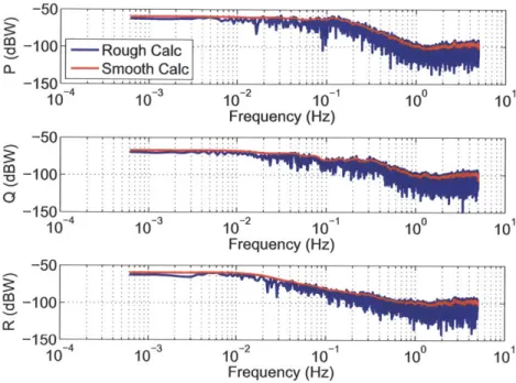
3.2.3 _{Spectral Analysis . . . .} 3.3 Control System Analysis . . . .

3.3.1 _{Linearized Plant Model. . . . .} 3.3.2 Nonlinear Plant Model . . . . 3.4 Open-loop Pointing Error Analysis . . . . 3.4.1 Problem Definition . . . . 3.4.2 _{Pointing Error Closed Form Analysis . . .} 3.4.3 Small Angle Pointing Error Approximation 3.4.4 _{Pointing Error Look Up Tables . . . .} 3.4.5 Open-loop Pointing Error Distribution . .

3.5 Open-loop Antenna Pointing Simulation . . . . .

3.5.1 Racetrack Flight Data . . . .

3.5.2 Cruise Flight Data . . . . 4 Closed-Loop Tracking

4.1 Effects on Signal-to-Noise Ratio . . . . 4.1.1 _{Received Isotropic Power . . . .} 4.1.2 Thermal Noise . . . .

4.1.3 _{Receiver Antenna Gain . . . .} 4.1.4 Military Satellite Communications Systems 4.2 Signal-to-Noise Ratio Characterization . . . . 4.2.1 _{Thermal Noise Power Characterization . .} 4.2.2 Received Isotropic Power Characterization 4.2.3 SNR Characterization . . . . 4.2.4 _{SNR Analysis . . . .} 4.3 _{Step-Tracking Algorithm . . . .} 4.3.1 Step-Tracking Theory . . . . . . . . 35 . . . . 35 . . . . 36 . . . . 38 . . . . 38 . . . . 38 . . . . 40 . . . . 44 . . . . 44 . . . . 49 . . . . 52 . . . . 52 . . . . 53 . . . . 56 . . . . 60 . . . . 64 . . . . 68 . . . . 68 . . . . 71 73 . . . . 73 . . . . 73 . . . . 78 . . . . 78 Characteristics . . 78 . . . . 79 . . . . 79 . . . . 83 . . . . 87 . . . . 89 . . . . 92 . . . . 92

4.3.2 Test Case Scenarios . . . . 4.3.3 Step-Tracking SNR Characterization . . 4.4 Closed-Loop Pointing Simulation . . . . 4.4.1 Ideal Pedestal Simulation . . . .

4.4.2 Closed-loop Pointing Simulation . . . . .

5 Conclusions and Suggestions for Future Work 5.1 Conclusions . . . .

5.2 Suggestions for Future Work . . . .

A Antenna Pedestal Equations of Motion

A.1 APS.nb . . . . A.2 Final Solution . . . .

B Matlab Simulation Code

B.1 Spectral Analysis . . . . B.1.1 SimSpectra.m. . . . . B.1.2 FreqAnalysis.m . . . . B.1.3 FreqSmooth.m. . . . .. B.2 Linearized Plant Simulation . . . .

B.2.1 SimLinear.m . . . . B.2.2 Linearized Plant Simulink Model . . B.3 Nonlinear Plant Simulation . . . .

B.3.1 SimNonlinear.m . . . . B.3.2 Nonlinear Plant Simulink Model . . . B.4 INS Error Simulations . . . . B .4.1 Pio.m . . . . B.4.2 PioAnalysis.m. . . . . B.4.3 INSErrorSim.m. . . . . B.4.4 INS Error Simulink Model . . . . B.5 Open-Loop Pointing Simulation . . . . B.5.1 Simulator.m . . . . B.5.2 Open-Loop Pointing Simulink Model B.6 SNR Characterization Simulations . . . . 117 . . . . . 117 . . . . . 117 . . . . . 118 . . . . . 119 .121 . . . . . 121 . . . . . 123 . . . . . 127 . . . . . 127 . . . . . 128 . . . . . 131 . . . . . 131 . . . . . 132 . . . . . 134 . . . . . 136 . . . . . 137 . . . . . 137 . . . . . 139 140 96 98 99 100 103 109 109 110 113 113 115 . . . . . . . .

B.6.1 B.6.2 B.6.3 B.6.4 B.6.5 B.7 Closed B.7.1 B.7.2 B.7.3 B.7.4 B.7.5 SimSNR.m . . . . SNR Characterization Simulink Model DistPlots.m . . . . SNRAnalysis.m . . . . SNRAnalysisII.m . . . . Loop Pointing Simulation . . . . AntPatt.m . . . . LookUpTable.m . . . . FullDitherSquintSim.m . . . . Closed-Loop Tracking Simulink Model DitherSquintSim.m . . . .

C List of Acronyms and Symbols

140 142 142 146 147 149 149 149 150 154 155 157

Chapter 1

Introduction

1.1

Motivation for Work

Satellite communication (SATCOM) systems provide beyond line-of-sight commu-nication with voice, video, and data capabilities. Although SATCOM applications are diverse, the U.S. military has realized the strategic and tactical advantage

SAT-COM systems can provide to troops in wartime environments, and has utilized this

technology in combat zones since the early 1990's [1, 2]. The Military Strategic and Tactical Relay (MILSTAR) program is one constellation of geosynchronous satellites within the Military Satellite Communications (MILSATCOM) system that provides secure beyond line-of-sight communication and enables sensitive information sharing between the President, the Secretary of Defense, and the U.S. Armed Forces around the globe [3].

MILSTAR is a robust "Nuclear Survivable" system with the ability to avoid, repel, and withstand virtually any enemy attack [4]. The MILSTAR satellites operate in the Extremely High Frequency (EHF) band, with center frequencies for downlink and uplink at 20 and 44 GHz, respectively. The system utilizes fast frequency hopping to create low probabilities of interception and detection [5]. The MILSTAR satellites operate in a protected protocol, so there is no tracking beacon for adversaries to locate and jam. At the same time, the lack of a beacon makes it difficult for allies to acquire and track the satellite.

SATCOM terminals point an antenna at an orbiting satellite to secure a

commu-nication link. Mobile SATCOM terminals perform the same function within either land-based or airborne vehicles and utilize system feedback to cancel out vehicle motion. An inertially stabilized platform cancels disturbances and keeps a payload within an inertial reference frame. A gimballed pedestal is a type of inertially stabi-lized platform that stabilizes and points an antenna in a specific direction [6]. The platform uses internal feedback to control the antenna's orientation and point it in the direction commanded by the pedestal control computer commands. The control computer calculates a pointing solution based on the satellite's location and the

ter-minal's location and orientation. This form of control is defined as open-loop pointing because the solution incorporates no performance feedback to reduce and eliminate errors within the pointing solution [7]. Errors enter the system and cause inaccuracies in the pointing solution, which reduce the received signal strength and decrease the communication link's performance. More robust systems utilize closed-loop tracking to improve the pointing performance by feeding back the received signal strength. Closed-loop tracking reduces bias errors in the pointing solution and improves the communication link.

Commercial terminals rely on feedback using continuous beacons to eliminate pointing errors. The lack of a beacon in protected transmission makes closed-loop tracking more difficult, but still possible. Airborne terminals have difficulty in point-ing due to aircraft disturbances and non-ideal system hardware. For protected air-borne terminal transmission, closed-loop tracking methods can be modified to re-duce uncertainty and eliminate an error from the open-loop pointing solution. If the method is modified improperly, closed-loop tracking may cause more error than reduce the error from open-loop pointing. The modified closed-loop tracking should reduce the uncertainty in feedback and eliminate any open-loop pointing error.

1.2

Problem Statement

MILSATCOM terminals for airborne applications require accurate pointing of the

antenna to achieve the best communication link performance. Pointing error biases in the open-loop pointing solution degrade performance and closed-loop tracking at-tempts to reduce this error. The goal of this thesis is to define relevant parameters that affect the terminal's pointing performance and analyze their impact on a com-munication link, which is accomplished by the objectives as follows:

1. Defining a nominal, two-axis gimballed antenna pedestal and developing an

open-loop pointing controller using state-space control techniques.

2. Obtaining a model for the open-loop pointing error from random errors in the

GPS/INS using statistical analysis and simulations.

3. Examining the performance of the open-loop pointing solution through

simula-tion.

4. Characterizing and modeling the received signal-to-noise ratio from the MIL-STAR satellite through simulation.

5. Defining a step-tracking algorithm that accomplishes closed-loop tracking and

eliminates pointing error in the presence of uncertainty in the received signal-to-noise ratio.

6. Examining the performance of the closed-loop tracking algorithm through

7. Determining the design constraints and system performance for different

hard-ware and their impact on open-loop pointing and closed-loop tracking perfor-mance.

1.3

Contributions

This thesis makes the following contributions while accomplishing the objectives out-lined in Section 1.2:

1. Analyzes inaccuracies in the open-loop pointing solution caused by random

errors in the attitude information from the GPS/INS Euler angle information. 2. Creates an open-loop pointing Simulink model that incorporates the dynamics

of the pedestal, the aircraft disturbances, and open-loop pointing solution errors.

3. Characterizes the average signal-to-noise ratio as a function of the number of

samples.

4. Creates a closed-loop tracking Simulink model that incorporates the uncertainty of the signal-to-noise ratio and pointing error from the open-loop pointing sim-ulation.

1.4

Thesis Overview

Chapter 2 explains the SATCOM system architecture and the hardware within a MILSATCOM terminal. Chapter 3 focuses on the open-loop pointing portion of the problem by first deriving the pedestal dynamics and an open-loop pointing controller

(Objective 1). The chapter then presents analysis on the open-loop pointing er-ror caused by random erer-rors in the GPS/INS Euler angle information (Objective 2).

Chapter 3 concludes by presenting simulations of the open-loop pointing performance in the presence of pedestal dynamics, aircraft disturbances, and open-loop pointing errors (Objective 3). Chapter 4 focuses on the closed-loop tracking portion of the problem and begins by defining the signal-to-noise ratio and modeling its uncertainty (Objective 4). The chapter continues by presenting a closed-loop tracking algorithm (Objective 5) and a simulation that tests the closed-loop tracking performance (Ob-jective 6). The chapter concludes with an analysis of the simulation results (Ob(Ob-jective

Chapter 2

Satellite Communication Terminal

Architecture

The design, fabrication, and implementation of a mobile satellite communication

(SATCOM) terminal must balance many different factors including mission

con-straints and system hardware selection. Mission concon-straints may limit the terminal to a certain size and weight. System hardware selection determines the level of attainable pointing accuracy, which in turn affects the communication performance. Engineers address all of these issues in mobile SATCOM terminal design. This chapter examines the the issues surrounding the different components of the mobile SATCOM terminal system hardware.

A SATCOM terminal contains all hardware and software required to stabilize and

point an antenna at an orbiting satellite and also to transmit and receive data. This thesis focuses on communication performance in the presence of non-ideal stabiliza-tion and pointing. Stabilizastabiliza-tion and pointing in the presence of aircraft disturbances are the functions of the Antenna Positioner System (APS). The APS is comprised of an antenna pedestal system, a Global Positioning System (GPS)/Inertial Navigation System (INS), satellite ephemeris, and a pedestal control computer. The signal pro-cessing system is a separate system that performs the terminal's transmit and receive functions. Figure 2-1 is a block diagram of the components of a SATCOM terminal and their connections. The following sections explain each component of the block diagram.

SATCOM Terminal

Antenna Positioner System

Signal

Processing

System

Figure 2-1: SATCOM terminal block diagram defines the Antenna Positioner System, Signal Processing System, their internal subsystems, and the connections between each system.

Figure 2-2: Antenna pedestal system contains the antenna and pedestal. The sys-tem passes the received signal to the signal processing syssys-tem and obeys pointing commands from the pedestal control computer.

2.1

Antenna Pedestal System

The antenna pedestal system consists of the antenna hardware and the pedestal required to point the antenna. Figure 2-2 is a picture of the antenna pedestal system used in this thesis.

2.1.1

Antenna

The antenna collects and directs RF energy between the satellite and the terminal to establish a communication link. In communication theory, an isotropic antenna emits and collects energy uniformly in three-dimensional space. In practice, a directional antenna focuses energy in a specific direction and the direction of maximum gain is defined as the antenna aperture's boresight. Apertures for EHF (30-300 GHz)

SATCOM applications are typically highly directional in order to transmit great

distances at high frequencies [8].

An antenna beam pattern characterizes the gain with respect to the antenna aper-ture's boresight and is used to define the pedestal's pointing performance requirement. Figure 2-3 is an example of a antenna beam pattern for a small aperture antenna com-monly used in SATCOM systems. The main beam is the region of the beam pattern between the first set of nulls and the side lobes are the successive decreasing lobes on either side of the main beam. The half-power beamwidth (HPBW) is the angle be-tween the two -3dB points and is a function of the aperture size and the transmission frequency. Most SATCOM systems require the pedestal to point at the satellite to within the antenna aperture's HPBW so that the received power does not drop below

0 - -.. -. -. -. -5 --10 -- - - -~-15 -- ---- --20 - - --25-- - - -N S-30- - -0 - 4 0 -- -... ... -... .-.-. -40 --50 -2 -1 0 1 2

Angle Off Boresight (0)

Figure 2-3: A one-dimensional cross-section of a 0.3 m radius aperture operating at 20 GHz. The antenna pattern is normalized to 0 dB and the red line defines the half-power beamwidth region.

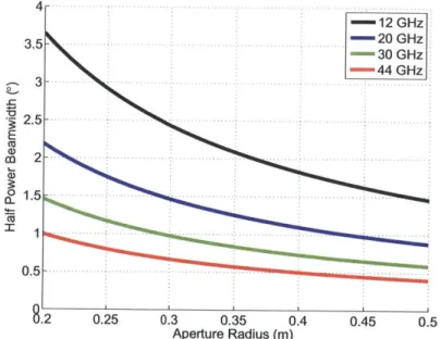
4--- 12 GHz 3 -20 GHz - 30 GHz -44 GHz -3 Ca 2 .. .... ... 1 .. .- . - -.. -- 1 .5 -. .... ... ... -.. 8.2 0.25 0.3 0.35 0.4 0.45 0.5 Aperture Radius (m)

Figure 2-4: Typical half-power beamwidths for various size apertures at different frequencies.

50%. Figure 2-4 demonstrates that as the antenna aperture size and transmission

frequency increase, the antenna beam's null-spacing decreases, which translates to tighter pointing requirement [9].

in order to steer the aperture's boresight toward the satellite. Fixed boresight an-tennas, such as a parabolic dish, must be physically moved to steer the boresight. They are typically mounted to gimballed pedestal systems, which enable them to point in any commanded direction. An electrically steerable boresight antenna, such as a phased array, is a much more advanced piece of hardware [9]. The reduction in moving parts makes electrically steerable boresight apertures more attractive to mobile SATCOM applications. However, the design effort is considerably greater, which significantly increases the system cost.

This thesis uses a fixed boresight aperture that transmits and receives at EHF. The transmission frequencies for downlink and uplink are 20 and 44 GHz respec-tively. An antenna with a fixed aperture is selected over a phased array to reduce the overall system cost. The antenna beam pattern in Figure 2-4 is the normalized one-dimensional beam pattern for a 0.3 m radius antenna aperture at the 20 GHz receive frequency. This thesis focuses on a 0.3 m dish, but also analyzes 0.4 and 0.5 m dishes to understand how performance changes for larger apertures. Each larger aperture has a smaller HPBW, which translates to a tighter pointing performance re-quirement. Because this thesis uses a fixed boresight aperture, it requires a multi-axis gimballed pedestal to steer the antenna's boresight.

2.1.2

Pedestal

A pedestal stabilizes and points a fixed boresight aperture in a commanded direction,

which requires a minimum of two axes of rotation. A gimbal is a collection of motors, bearings, and machined parts that forms a rigid body and allows motion in one axis of rotation [6]. The two-axis gimballed system is the simplest, cheapest, and sturdiest configuration that points an antenna in any direction. The outer gimbal controls the azimuth axis, while the inner gimbal controls the elevation axis. The set of gimbals provide a complete range of motion in a hemispherical field of view from horizon to zenith and steer the antenna's boresight any direction within that range.

The only disadvantage to a two-axis system is the problem of gimbal lock, which occurs at elevation angles approaching zenith. When the elevation gimbal is directly at 900, the system reaches a singularity, which causes the pedestal to have only one degree of freedom instead of the normal two degrees of freedom. This reduction in axes of rotation imposes no problem in a static tracking problem, but becomes a major concern in a dynamic tracking problem. With dynamic azimuth and eleva-tion commands coming from the pedestal control computer, it becomes increasingly difficult to control the azimuth gimbal at high elevation angles because the required azimuth rate of change approaches infinity.

The problem occurring at zenith is averted by avoiding any elevation angle above

800 , which is commonly referred to as the keyhole region due to the hole in the

pedestal's field of view at zenith [9]. Another option, if operation in or near the keyhole region is required, is to have a third gimbal that eliminates the singularity and the gimbal lock constraint. A third gimbal also increases the size, complexity,

and cost of the system. Debruin [9] discusses pedestals with three degrees of freedom and their possible configurations in more detail.

In addition to pointing the antenna in any desired direction, the pedestal also cancels out disturbances and stabilizes the pedestal. Torque disturbances enter the gimballed pedestal and cause unwanted angular accelerations in the axes of rotation resulting in pointing error [6]. These disturbances are caused by coulomb friction, spring torques, imbalance, vehicle motion coupling, intergimbal coupling, internal disturbances, structural flexure, and environmental disturbances [10]. Sensors mea-sure these unwanted rotations and the pedestal then uses the gimbal motors to cancel out the torque disturbances.

The pedestal uses gyroscopic sensors and angular resolvers to sense these un-wanted rotations. A gyroscope measures rotational acceleration in inertial space and is typically aligned and mounted with the antenna's reference frame. The pedestal is then able to detect any accelerations the antenna experiences and counteract them with torques in either gimbal. Position resolvers attached to each gimbal feed back orientation data to the pedestal so that any errors between the commanded and actual angles are eliminated. The pedestal system characterized in this thesis utilizes a 2-axis gimballed system to point the antenna because the mission profile does not require keyhole operation based on the aircraft's flight dynamics and area of operation.

Internal to the two-axis pedestal for this thesis, Cleveland Motion Controls (CMC) 2100 series brush servo-motors with F-windings are the steering motors for both gimbals. They have proven to be reliable in other APS projects conducted at Lincoln Laboratory [11]. The EHF SATCOM On-The-Move project mounted an APS on a High Mobility Multipurpose Wheeled Vehicle (HMMWV) and required accurate pointing in the presence of severe vehicle motion in off-road environments [12]. In this thesis, the disturbances from the airborne environment are less, but the operating environment is harsher due to the extreme cold at altitude.

The feedback sensor for the pedestal in this thesis include angular resolvers for each gimbal and a two-axis KVH Industries fiberoptic gyroscope mounted to the inner gimbal to measure rotational accelerations in the pitch and yaw axes [13]. These measurements are fed back internally to the pedestal to ensure that it points where it is commanded. This commanded input comes from the pedestal control computer after it calculates a pointing solution. This calculation requires information on the pedestal's current position, velocity, and orientation. This knowledge comes from the

- (S9. 0 L n)

Figure 2-5: GPS/INS block contains the GPS/INS hardware and transmits the sys-tems location and orientation to the pedestal control computer.

2.2

Global Positioning System/Inertial Navigation

System

The Global Positioning System/Inertial Navigation System (GPS/INS) subsystem transmits the system's location and orientation to the pedestal control computer. Figure 2-5 is a picture of this subsystem. This section explains the theory behind both the INS and GPS and why they are combined into one subsystem.

2.2.1

Inertial Navigation System

Many vehicles, including some aircraft and submarines, use an Inertial Navigation System (INS) to provide position and attitude information. To determine positions, an INS measures accelerations using three orthogonal accelerometers. The acceler-ations are integrated once to obtain inertial velocity, and a second time to obtain position relative to the Earth. Because the vehicle attitude changes over time, the orientation of the accelerometers relative to the navigation frame must be determined. Early versions used an inertially stabilized platform, which uses gyroscopes on the platform and an actuated gimbal system to maintain the accelerometers in a fixed direction in the navigation frame. In more modern strapdown systems, the accelerom-eters are fixed relative to the vehicle frame, and measured angular rates are integrated to determine the relative orientation of the vehicle and navigation frames [14,15].

When doing computations in a strapdown INS, several choices of coordinate sys-tems are possible. In this thesis, we will use the North, East, and Down (NED) reference frame. The origin of the NED reference frame is located at a specific point relative to the INS. The Z-axis points down; the X- and Y-axes point North and East, respectively, so that the three axes form an orthogonal basis. Note that the

NED frame is not an inertial frame, because its orientation in inertial space changes

as the Earth rotates, and as the vehicle moves over the surface of the Earth. Nev-ertheless, in some references, the NED frame is treated as an inertial frame, because the angular rate of rotation of the coordinate system with respect to inertial space is significantly smaller than the angular rate experienced by the vehicle [16].

In principle, a strapdown INS with ideal accelerometers and gyroscopes and per-fect knowledge of the vehicle initial conditions can determine the vehicle position with perfect accuracy. In practice, the inertial measurements are subject to numerous er-rors, including scale factor erer-rors, misalignments, and random noise, and the initial conditions are known imperfectly. As a result, the navigation errors of an INS tend to grow over time. The errors can be reduced by incorporating information from other types of navigation systems, such as the Global Positioning System, discussed below.

2.2.2

Global Positioning System

The Global Positioning System (GPS) is an alternative navigation system used in other vehicles such as cars or boats. A constellation of satellites orbiting the Earth make up the GPS network. Each satellite transmits RF energy signals with time-stamped data. Once this data is decoded by a receiver, the data gives the total travel time between satellite and receiver and can then be converted into an estimated range. With a minimum of four satellites in view, the receiver can triangulate its position with a certain degree of precision. Calculating a position requires three range measurements, synchronization errors among the satellites and the receiver cause the measurements to only be approximations of the range (pseudorange). A fourth pseudorange measurement eliminates the synchronization issue [17,18].

The receiver estimates its position, using a Kalman filter, with higher precision as more satellites are in view. Gaps in the constellation or obstruction in the time-stamped signal can cause the number of measurements to drop below the minimum, resulting in a blackout. The system always stores its last calculated position, but can only extrapolate its next position using calculated velocity vectors prior to the blackout period. The risk of blackout is not an issue for a steady vehicle with little change in orientation. On the other hand, a blackout could be a very serious issue during critical maneuvers that require real-time position and orientation information, such as landing or refueling an aircraft.

2.2.3

GPS/INS Integration

GPS provides an accurate position, but only updates once per second. An INS

mea-sures changes in position and orientation at a much higher rate, but accumulates error and drift. Combining the GPS and INS into one system provides accurate posi-tion and orientaposi-tion informaposi-tion. The combinaposi-tion makes up for the shortcomings of each separate system [15]. A Kalman filter optimally blends the two systems in the presence of noise and uncertainty.

A few methods of integration that are commonly used in navigation systems are

loosely-coupled, tightly-coupled, and ultra-tightly coupled [19, 20]. Loosely-coupled integration takes the GPS solution and filters it with the INS solution to bound the drift. Loosely-coupled systems utilize two separate Kalman filters in cascade: a Kalman filter in the GPS, and a separate filter that takes the position output and blends it with the INS solution.

Tightly-coupled integration combines the two Kalman filters from the loosely-coupled such that the raw pseudorange measurements from the GPS receiver feed directly into the Kalman filter along with the IMU data. This scheme is more robust in the presence of signal blockage or too few satellites being in view [21, 22].

Ultra-tightly coupled integration is much more advanced than the other two schemes. Strategic navigation systems in wartime environments utilize this integra-tion method in the presence of jamming and interference. The ultra-tightly coupled integration method attempts to mitigate jamming and interference by designing the

Kalman filter to utilize the in-phase and quadrature samples from the GPS receiver. Unlike pseudorange measurements, these samples are less susceptible to malicious tampering [23]. Each level of integration increases the precision, but also increases the design complexity and system cost.

The APS within this thesis utilizes a tightly-coupled GPS/INS receiver. The tightly-coupled integration is selected over the other two options because it provides an accurate solution in the presence of blackout and the mission profile does not re-quire the GPS/INS system to operate under jamming and interference. The GPS/INS supplies the APS with accurate knowledge of the system's current location and ori-entation, so the control computer can calculate a pointing solution.

z

h

hy Y

Ascending node

X~0.

Figure 2-6: Satellite ephemeris contains orbital parameters that define the satellite's location at specific instance in time, which the computer can then use to estimate future target coordinates. Reproduced from Reference 24.

2.3

Satellite Ephemeris/Target Location

The pedestal control computer requires an accurate knowledge of the satellite's loca-tion in order to calculate a pointing soluloca-tion between the terminal and the satellite. Satellite ephemeris pinpoints the satellite's exact location at a given instance in time and can then be used to estimate future positions in time. Figure 2-6 is an illustration of the satellite's location information contained in ephemeris.

2.3.1

Satellite Orbital Characteristics

In order to know the satellite's location, it is useful to understand the physics behind satellite orbits. Equations of motion describe a satellite's trajectory around the earth.

These equations require six orbital elements, which define the satellite's orbit and its location in the orbit. Figure 2-6 presents the six orbital elements. Once these elements are known for a given instance in time, computers use orbital propagation algorithms to estimate the satellite's trajectory and future position.

Over time, orbital perturbations cause the orbital paths of each satellite to change, creating an error between the true and estimated positions. Atmospheric drag, the Earth's oblateness, solar radiation pressure, and third-body gravitational effects are common perturbations experienced by satellites [25]. Physically changing the orbit or updating the orbital parameters to reflect the new, perturbed orbit are two methods to reduce the error between the estimated and true position.

Engineers take orbital perturbations into consideration when designing a satellite for a specific mission and install hardware on the satellite to reduce or eliminate perturbations the satellite may encounter during its life span. Engineers track the satellite's orbit, and can command the satellite to use onboard hardware, such as a propellant tank or stabilization gyroscope, to get it back in its desired position and orientation [25]. If onboard hardware cannot correct for the perurbation, then the satellite's ephemeris is updated to account for this change.

2.3.2

Satellite Ephemeris

The calculation of a satellite's ephemeris uses high fidelity orbital propagation al-gorithms to account for predictable perturbations, but cannot account for random perturbations. To account for random perturbations, tracking stations observe and record all perturbations in a satellite's orbit and routinely update the ephemeris by transmitting it to the satellite. Updating the ephemeris helps ease acquisition, be-cause the satellite can either broadcast it continuously or transmits it to a user after receiving a request [17]. Uncorrected ephemeris only poses a serious threat if the system is unable to calculate the satellite position well enough to establish a com-munication link. Once the link is established, the ephemeris can be updated and the terminal will have the best estimate of the satellite's location.

2.3.3

Geostationary Orbits

Satellite orbits are classified based on their shape, direction, or altitude. Satellites fall into one of three altitude ranges: low earth orbit (LEO), medium earth orbit (MEO), and geosynchronous earth orbit (GEO). Satellites are considered LEO if their altitudes are less than 1000 km and satellites with an altitude of exactly 35,786 km are GEO. Satellites with an altitude between 1000 and 35,786 km are categorized as MEO [26].

GEO satellites have the unique trait of a 24 hour orbital period. To an observer

on the Earth's surface, a GEO satellite appears to make a figure-eight pattern in the sky. If a GEO satellite has an inclination of 00, so that it orbits the Earth along

its equatorial plane, then the satellite is in a geostationary orbit, which means the satellite would appear as a fixed point in the sky. Geostationary orbits are commonly used by communication satellites to eliminate the added complexity of pointing at a moving target. MILSTAR satellites operate in geostationary orbits.

Besides the reduction in acquisition and tracking, GEO satellites at such a high altitude have a very wide area of coverage. A GEO satellite can see nearly a fourth of the Earth's surface, and can transmit very wide or narrow beams depending on the mission parameters or even multiple beams to allow for different coverage areas at different transmission rates. Additionally, the Doppler effect is not a significant issue because the satellite is stationary relative to the Earth's surface and there is little to no change in relative motion between the satellite and terminal, even in an airborne application [8].

GEO satellites operate at such a high altitude that signal attenuation and

trans-mission delays can be a problem. Attenuation is a function of the transtrans-mission fre-quency and the distance the signal travels. Section 4.1 discusses this in more detail as it is related to the Received Isotropic Power (RIP). RF signals propagate at the speed of light, which means a signal takes approximately 120 ms to travel between antennas. This propagation delay may present a serious issue if the mission requires real-time communications.

Orbital perturbations cause GEO satellites to move from their fixed position above the Earth. Atmospheric drag does not affect GEO satellites because they operate

25,000 km above the atmosphere. At this extreme distance away from the Earth,

the orbit's eccentricity and inclination change over time. Solar-radiation pressure causes long term variations in eccentricity, while third-body gravitational effects from the Sun and Moon cause long-term variations in inclination. In addition, tesseral harmonics induced by the Earth's gravitational field cause longitudinal shifts in the satellite's position over the Earth [27].

Scientists have documented each of these perturbations, and engineers take them into consideration when designing the satellite. Most GEO satellites mitigate these errors and maintain their intended orbit and fixed location in the sky. In addition, satellite operators track the satellite's performance and take the necessary actions to ensure the satellite follows its intended orbit. As stated previously, the ephemeris reflects all perturbations and changes in the satellite's orbit and should give the best possible estimate of the satellite's location.

Figure 2-7: Pedestal control computer interacts with all of the other subsystems within the APS as well as the Signal Processing System. The computer is responsible for calculating the pointing solution and performing closed-loop tracking.

2.4

Pedestal Control Computer

The pedestal control computer, presented in Figure 2-7, takes the terminal position and orientation data from the GPS/INS and the satellite ephemeris and calculates a pointing solution. The computer then commands the pedestal to steer the antenna's boresight in the direction of the pointing solution. Feedback internal to the pedestal controls the gimbal orientations. This feedback is defined as open-loop pointing, be-cause the system does not utilize feedback from the terminal to improve the pointing solution. The pedestal control computer performs closed-loop tracking by manipu-lating the received signal level to eliminate pointing error biases from the open-loop pointing solution.

Open-loop pointing is the simple solution to the pointing problem, but cannot de-termine the amount of pointing error between the terminal and the satellite. Closed-loop tracking provides a more robust solution that eliminates open-Closed-loop pointing errors, but decreases performance temporarily and could potentially decrease overall system performance. The concerns of each are discussed in this section and Chap-ters 3 and 4 study the trade-offs in more detail.

2.4.1

Open-Loop Pointing

Open-loop pointing receives information on the target's location and the terminal's position and orientation, calculates a pointing solution, and commands the pedestal to point in the calculated direction. Several early SATCOM systems performed open-loop pointing with great success [28,29]. The fundamental problem with open-open-loop pointing is that there is no way to eliminate an error in the open-loop pointing solution. This open-loop pointing error is a summation of several smaller errors within the pedestal that impact the final pointing solution. The errors include

1. Aged satellite ephemeris at the terminal.

3. Misalignment errors between components.

4. Steady-state biasing in pedestal resolvers.

Aged satellite ephemeris causes error in the satellite's estimated position. Pertur-bations in the satellite's orbit cause the satellite's position to be different from the estimated position. Aged ephemeris does not account for more recent perturbations and could potentially estimate an incorrect satellite location. Aged ephemeris is only an issue in the acquisition phase of the communication link. Once the terminal has acquired the satellite, it can request updated ephemeris, which is then stored in the pedestal computer's memory. The impact of aged ephemeris is reduced for geosta-tionary orbits because the satellite appears as a fixed point in the sky. Additionally, the distance between the terminal and satellite is great, which means errors in the satellite's position translate to infinitesimal error angles.

A much more serious error stems from inaccuracies in the GPS/INS solution.

Noisy sensors within the INS cause errors to accumulate over time. Integrating the output with the GPS bounds the drift and reduces the error. GPS/INS hardware specifications define the position and orientation errors as Gaussian random variables with defined variance. Similar to the satellite position error, errors in the termi-nal's position do not cause serious errors in the pointing solution. On the other hand, orientation errors factor directly into the pointing solution [30]. The amount of point-ing error in the open-loop pointpoint-ing solution is tied directly to orientation error and are analyzed further in Section 3.4. Misalignment between the sensors causes non-orthogonality in the system. If one sensor is misaligned, then it senses acceleration in an axis other than the intended axis, which causes an error in the system's reported orientation. Navigation grade GPS/INS are put through rigorous tests to ensure the sensors are indeed orthogonal.

Unmeasured misalignment errors in any of the components cause an error in the pointing solution. Misalignment errors are either static or dynamic. Mounting mis-alignment errors cause static biasing errors between components, while bending and flexing of the aircraft frame cause dynamic misalignment errors. Static errors are mitigated by paying extra attention to accurate mounting and alignment. If the

GPS/INS is far enough from the pedestal, flexing of the aircraft could cause dynamic

errors. Mounting the GPS/INS to the base of the pedestal mitigates this error. Mis-alignment errors can also exist internal to the pedestal or between the antenna and the pedestal. All of these misalignments are factors directly influencing the pedestal's pointing accuracy and the terminal's communication performance. It is assumed that the careful design of the antenna pedestal minimizes these errors.

The final form of error is steady-state biasing in the pedestal resolvers. This bias results in an error between where the pedestal is commanded to point and where it actually points. This bias will cause a significant error not in the pointing solution, but in the pedestal pointing accuracy. The most effective method to eliminate this error is through careful design and calibration.

2.4.2

Closed-Loop Tracking

The pedestal control computer performs closed-loop tracking by calculating the same pointing solution as before and then using the received signal-to-noise ratio to detect any error in the current pointing solution. Three closed-loop tracking strategies are commonly used in radar and communication systems.

1. Monopulse

2. Conical Scanning

3. Step tracking

Monopulse tracking uses multiple antennas to locate and track a target. The signal levels from the individual antenna feeds are manipulated to determine a pointing offset between the antenna and the target. The pointing solution is updated with the calculated pointing error [31, 32]. When the signal levels from all of the feeds are equal, the main beam is accurately pointed at the target. Monopulse tracking is more commonly found in radar tracking systems than communication systems because they require advanced hardware, with multiple antenna feeds. The antenna within the MILSATCOM terminal has only one feed. For this reason, monopulse tracking is not a viable solution.

Conical scanning, conscan for short, is a technique common to both radar and communication systems. Instead of using multiple feeds as monopulse tracking does, conscan requires only one antenna feed. The antenna aperture's beam is mechanically steered in a circular motion around the estimated pointing angle. The circular motion causes sinusoidal variations in the received signal power, which are then used to esti-mate the pointing error. This estiesti-mated error is fed back into the pedestal as gimbal orientation corrections [33]. The radius of the conscan movement is selected based on the antenna pattern so no significant loss in signal power occurs. The sinusoidal fre-quency is chosen based on the system's sampling rate. Other more elaborate scanning patterns, such as the Lissajous and rosetta pattern, have been designed and tested and present similar results [33]. Conscan tracking can be very useful, but it may require extra equipment. The pedestal control computer can command the pedestal to manually steer the antenna or the feed within the antenna can be off-centered and rotated. The latter requires more equipment and increases the system's complex-ity and cost. Furthermore, conscan tracking works best in systems with continuous beacon. For protected systems, uncertainty in the signal-to-noise ratio degrades the performance of the conscan tracking algorithm and the continuous motion of conscan tracking degrades communication performance.

The simplest and least expensive method for closed-loop pointing is step tracking, which has some of the advantages of both monopulse and conscan techniques. Step tracking requires only one feed, so no modification to the antenna is required. In addition, step tracking does not require any augmentation to the pedestal to scan the antenna beam. Step tracking takes SNR readings at specific points in a desired

pattern and then adds and subtracts the samples to estimate the pointing error, which the computer then uses to recalculate the pointing solution. The difference between step tracking and conscan is that step tracking points at a fixed location in the sky and takes enough samples to estimate the SNR rather than continuously scanning the antenna. This thesis focuses on step tracking because it is the most practical form of closed-loop tracking for protected MILSATCOM transmission.

Chapter 3

Open-Loop Pointing

3.1

Plant Definition

The purpose of this section is to define the plant model of the pedestal by character-izing the dynamics of a two-axis gimballed system and the dynamics of the attached motors.

3.1.1

Equations of Motion

The equations of motion describe the system's response to internal and external forces. The response side of the equation, typically the left hand side of the equation, defines the internal interactions within the system, while the moment side, the right hand side, defines the external torques acting on the system. The derivation of the equations of motion is commonly available for a standard rotating rigid body and explicit definitions of both sides of the equation are commonly available [16]. The two-axis gimballed pedestal is not a rigid body because of its two axes of rotation. Therefore a more rigorous derivation is required to solve the equations of motion that govern a two-axis gimballed pedestal.

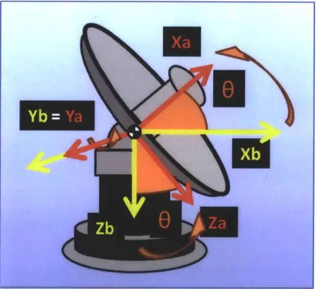
The antenna pedestal houses a two-axis gimballed system as depicted in Figure

3-1. The two degrees of freedom allow the pedestal to point the antenna in any direction

within the pedestal's hemispherical field of view. The azimuth and elevation gimbal angles, represented by V4 and 0 respectively, define the orientation of the APS.

Three reference frames describe the orientation of the three pedestal components. These define the rotation transformation from the aircraft frame to the antenna body frame. In addition to the aircraft reference frame, denoted by [Xk, Yk, Zk], the other

two frames are fixed to the azimuth and elevation gimbals within the system, and are

denoted by [Xb, Yb, zb] and [xa, ya, za], respectively. Figure 3-1 graphically defines each

reference frame.

an-Figure 3-1: The antenna pedestal two-axis gimballed system contains three reference frames. [Xk, Yk, Zk] is fixed to the base of the pedestal and is aligned with the aircraft

reference frame. [Xb, Yb, Zb] is fixed to the azimuth gimbal and serves as the transition

frame. [xa, ya, za] _{is fixed to the elevation gimbal and is aligned with the antenna's}

Figure 3-2: The azimuth gimbal rotation about the Z-axis by azimuth angle /. The

rotation transformation from [Xk, Yk, Zk] to [Xb, Yb, Zb] is the relation between the air-craft frame and the transitional frame.

other. The transformation matrices from the aircraft frame to the azimuth frame by the angle V) and the azimuth frame to the elevation frame by the angle 0 are defined as cos(4) sin() 0 Rbk - sin(O) cos(4) 0 (3.1) 0 0 1 and [cos(9) 0 - sin(9) Rab 0 1 0 (3.2) L sin(9) 0 cos(0)

respectively. Figures 3-2 and 3-3 depict the two rotations about angles

4

respectively.

An angular rotation in one frame is related to an angular rotation in another frame

by one of the transformation matrices. This angular rotation depends on the azimuth

and elevation gimbal orientations as well as the gimbal angular velocities [34]. The angular velocities for the three reference frames are defined as

Pk

Wk qk , (3-3)

Figure 3-3: The elevation gimbal rotation about the Y-axis by elevation angle 0.

The rotation transformation from [Xb, Yb, Z] to [Xa, Ya, Za] is the relation between the

Pb Wb = qb (3.4) Tb and Pa Wa = qa

,

where p, q, r represent the roll, pitch and yaw components in each frame, respectively. The relationships between the angular velocities and their respective reference frames are given by

Pb Pk cos(0) + qk sin14>)

qb -Pk sin(o) + q cos(V) (3.6)

_Tb _ k +

and

[Pa

1

1

qa =, q+0 (3.7)

[a

I

where ?/ and 2b are the angle and angular rate of the azimuth gimbal and 0 and 0 are the angle and angular rate of the elevation gimbal [34].

The two axes of concern in this application are the pitch and yaw velocities (qa

and Ta) of the elevation gimbal because unwanted rotations in these axes correspond to pointing error between the antenna and the satellite. Because the antenna aperture is circularly symmetric, no orientation requirement exists between the terminal and satellite, so rotation in the roll axis does not impact performance. Any deviation in either the pitch or yaw axis will result in a pointing error and a loss in signal strength, and so the pedestal is designed to eliminate these rotations.

The standard equations of motion for a rigid body cannot describe the antenna pedestal because it can rotate in two axes. The gimbals within the pedestal are rigid bodies, so the standard equations of motion describe the dynamics of each gimbal. Each gimbal has an inertia matrix associated with it that is defined by

IXX IXY IXZ~

I = IXY IYY IYZ (3.8)

IXZ IYZ Izz_

where

(Ixx,

(Iy,

inertia. The moments indicate the rigid body's resistance to rotation about each axis and the products indicate the cross-coupling and symmetry of the body [16].

The equations of motion of a rigid body define the angular velocities and acceler-ations caused by torques entering the system and interacting with the inertia matrix

as indicated by

1. + w x Iw = T, (3.9)

where c, w, and T are the angular acceleration, angular velocity, and external torque. As defined earlier, the left hand side contains the response and the right hand side contains the external torques. The fully derived equations of motion with all angular velocities and accelerations are

[

+

₊

-TX)I

1

F

]

4_{Iy - pr(Iz - Ix) +}

(p2 _{- r}2_{)Ix; - (rq -}

₊

J

[

. (3.10)

H'Iz + pq(Iy - Ix) - (p2

- q2)Iy - (pr + )Iyz + (qr - )Ixz TZ

Equation 3.10 is the standard equations of motion for a rotating rigid body [16].

3.1.2

Elevation Gimbal

The elevation gimbal is isolated from the rest of the system and treated as a rigid body that contains both the gimbal and the mounted antenna. The standard equations of motion from Equation 3.10 characterize the dynamics of this subsystem. The derivation makes a simplification that reduces the complex cross-coupling among the three axes. Setting the products of inertia equal to zero cancels out the last three terms on the left hand side of Equation 3.10. This substitution is a reasonable simplification often done in practice because the source of the coupling is understood and engineers design systems with the inertia matrix in mind. This practice is done so that the final system is balanced with minimal cross-coupling between the axes. Pedestal designs follow this practice, so the resulting equations of motion for the elevation gimbal are defined by

Iaca + W. X lawa = T, (3.11)

which simplifies to

pa'xa + qara(Iza - ITa) TXa

4alya -para(Iza - Ixa) Ty . (3.12)

'aIza + paqa (Iya - Ixa) Tza

Coupling still exists among the three axes so most texts go a step further and eliminate the cross-coupling by linearizing the equations of motion around an operating point, such as straight and level flight [16]. This derivation incorporates the cross-coupling to more accurately characterize the dynamics and interactions within the pedestal.

The elevation gimbal controls rotation in the Y-axis by angle 0 as indicated by Figure 3-3. Tya in Equation 3.12 represents the external torque the gimbal exerts on the system to cause rotation in the pedestal's elevation axis. Txa and Ta are external torques the elevation gimbal cannot control, but still affect the gimbal and cause rotations in the yaw and roll axes of the elevation gimbal. All three torques define the interaction between the azimuth and elevation gimbal.

3.1.3

Azimuth Gimbal

The azimuth gimbal is another rigid body, so Equation 3.10 also characterizes the dynamics of the azimuth gimbal, but the right hand side of the equation is a little more complex because of the interaction between the two gimbals. The new right hand side includes the torques imposed directly on the azimuth gimbal as well as the torques from the elevation gimbal after a proper rotation transformation. The equations of motion of the azimuth gimbal are defined by

IbJb + Wb X IbWb = Tb - R- 1Ta, (3.13)

which fully expands to

Abxb + qbrb(Izb - Jyb)

[x

dblyb - Pbrb(Izb -- Ixb) Ty b -R Tya (3.14)

Lblzb + Pbqb yb- xb) Tb a

The azimuth gimbal controls rotation in the Z-axis by angle V as indicated by Fig-ure 3-2. Tzb in Equation 3.14 represents the external torque the gimbal exerts on the system to cause rotation in the pedestal's azimuth axis. Txb and Tyb are external torques the azimuth gimbal cannot control. These torques along with the torques from the elevation gimbal cause rotations in the roll and pitch axes of the azimuth gimbal. All of the external torques imposed on the pedestal come from the aircraft's angular velocities and accelerations, Pk, qk, rk and Pk, dk, ?k respectively.

3.1.4

Pedestal Dynamics

Equations 3.11 and 3.13 characterize the dynamics of the pedestal, but do not convey the relationship between the inputs and outputs very well. Equations 3.6 and 3.7

are substituted into Equations 3.11 and 3.13 to solve for the angular accelerations in

both gimbals as a function of the other parameters. After some simplification, the

equations for the elevation and azimuth gimbals are

I

= _{(To + (Iza - Ixa) Para)}

-4b _(3.15)

ya and

+

respectively, where

IZ Izb + Ia sin 2(0) + Iza cOs2(0)

Idl = [Ixb + Ixa cos2 (0) + Iza sin2 (0)1] Pbb (3.17)

Id2 = (Ixa - Iza) sin(20)(b - qbrb)